© The Authors 2025

1 Introduction

Massive stars (M_init ≳ 8 M_⊙ ) and their stellar winds play a crucial role in the chemical enrichment of galaxies (e.g., Portinari et al. 1998), not only by ionizing the interstellar medium (ISM), but also by enriching the ISM with nuclear processed material. The strong, UV-dominated radiation field drives a powerful stellar wind by transferring momentum from photons via absorption and scattering in metal line transitions (e.g., Castor et al. 1975; Pauldrach et al. 1986). Before ending their lives, some massive stars can completely deplete their hydrogen, even in their outer layers, and become a “stripped” helium star. This stripping can happen via strong, intrinsic stellar winds (Conti 1975; Abbott & Conti 1987), binary interaction (Paczyński 1967; Shenar et al. 2020; Dsilva et al. 2020), or eruptive events (Smith 2014). Stars characterized by spectra that are dominated by strong, broad emission lines, are classified as Wolf-Rayet (WR) stars (named after Wolf & Rayet 1867). If these stars are also He-burning and usually coinciding with highly depleted or absent hydrogen envelopes, they are called “classical”¹ WR (cWR) stars (e.g., Moffat 2015; Shenar 2024).

Developing accurate stellar atmospheres to reproduce the spectra of WR stars is vital to our understanding of the underlying physical processes inherent in these massive stars. Due to their intense radiation, low densities, and supersonic velocity fields, typical assumptions such as local thermodynamical equilibrium (LTE) cannot be applied; furthermore, the radiative transfer needs to account for specific line transitions as well as the expanding atmosphere, which is numerically challenging (see e.g., Hillier 2003; Hubeny & Lanz 2003; Hamann & Gräfener 2003). Consequently, non-LTE (NLTE) atmosphere modeling for the spectral analysis of O, B, and WR stars can essentially be performed only via 1D stationary models (see, e.g., Puls 2008; Sander 2017), typically solving the radiative transfer equations in the comoving frame (CMF), using state-of-the-art expanding atmosphere codes such as CMFGEN (Hillier & Miller 1998), PoWR (Gräfener et al. 2002), and FAST-WIND (Puls et al. 2005). A recent overview and analysis method comparison for O stars is given in Sander et al. (2024).

Despite the existence of modern model atmosphere codes, understanding cWR stars has turned out to be particularly challenging. One of the reasons is the so-called “WR radius problem,” referring to significant inconsistencies between the empirically inferred stellar radii and the predictions from stellar structure models (see, e.g., Hamann et al. 2006; Gräfener et al. 2012). Traditionally, the wind regime in atmosphere models used for quantitative spectroscopy is described by adopting a β-law velocity profile. For stars with dense stellar winds, the full emerging spectrum, including the continuum, is produced in the outer wind, leading to a significant parameter degeneracy with respect to the inferred radii (see, e.g., the discussion in Hamann & Gräfener 2004), which becomes even larger when allowing for different β values (Lefever et al. 2023). As demon-strated by Gräfener & Hamann (2005) and later also Sander et al. (2020) and Poniatowski et al. (2021), the radius problem can in principle be resolved if the velocity and density stratification are instead calculated in a consistent way based on the hydrodynamic equation of motion. Fully hydrodynamic models are thus likely crucial with respect to improving our understanding of the stellar atmospheres and spectra of WR stars. The concept of 1D hydrodynamically consistent CMF models goes back to Pauldrach et al. (1986), and it was first applied to WR stars in Gräfener & Hamann (2005, 2008). Subsequently, a dedicated hydrodynamically-consistent PoWR branch (PoWR^HD) was developed (Sander et al. 2017, 2023) and this is the approach we employ in this work.

Pioneering works on time-dependent, multidimensional, radiation-hydrodynamical (RHD) simulations with a hybrid opacity approach (Moens et al. 2022b; Poniatowski et al. 2022) for cWR stars were carried out by Moens et al. (2022a), later extended to the O star regime by Debnath et al. (2024); ud-Doula et al. (2025). Furthermore, Moens et al. (2022a) presented three cWR atmosphere models with luminosities of log L/L_⊙ = 5.47, 5.64, and 5.74 (termed Γ2, Γ3, and Γ4, respectively). These RHD models launch an optically thick supersonic wind from deep, sub-surface regions and are initiated due to the (hot) iron opacity peak. A fourth, lower luminosity model (log L/L_⊙ = 5.33, denoted as Γ1) from Moens et al. (2022a) includes instead a more standard, line-driven wind launched from higher, optically thin atmospheric layers.

In the first paper of this series (González-Torà et al. 2025), we compared the multidimensional RHD models by Debnath et al. (2024) with “standard” 1D PoWR models, constraining the (quasi)hydrostatic regime and a β-law to describe the stellar wind region. González-Torà et al. (2025) demonstrated that the inclusion of a turbulent pressure in the solution of the hydrostatic equation accurately reproduces the averaged density from the 2D models by Debnath et al. (2024). The velocity and partially also the temperature stratification were reproduced reasonably well, even when only assuming a constant turbulent velocity throughout the atmosphere. However, these models were limited to O stars, where 1D hydrodynamic results can be reasonably well approximated by a β-law (e.g., Gräfener & Hamann 2008; Hamann et al. 2008)². In this work, we shift the focus to WR stars and compare the 3D model results for the three highest luminosity cWR stellar models from Moens et al. (2022a) with new 1D hydrodynamically consistent PoWR^HD model calculations.

This paper is organized as follows: In Section 2 we present the main characteristics of the hydrodynamically-consistent 1D models with PoWR^HD and highlight the main differences compared to the stratification derived in the multidimensional hydrodynamical framework. Section 3 shows the profile comparisons for both modeling approaches and discusses the implications of our results. We present our conclusions in Section 4.

2 Methods

2.1 The PoWR ^HD 1D model

The Potsdam Wolf-Rayet stellar atmosphere code (PoWR, Gräfener et al. 2002; Hamann & Gräfener 2003; Sander et al. 2015) solves the CMF radiative transfer equations for a 1D spherical, stationary outflow. The non-LTE population numbers are calculated assuming statistical equilibrium (e.g., Hamann 1986) and the temperature stratification was obtained from a generalized Unsöld-Lucy method (Hamann & Gräfener 2003) or the thermal balance of electrons (Kubát et al. 1999; Sander 2015).

The inner boundary in PoWR models was set at a fixed Rosseland continuum optical depth, τ_Ross,cont. Both the radius, R_∗, and temperature, T_∗, are defined at the same τ_Ross,cont, thereby differing from the usual effective temperature, T_eff, definition at τ_Ross = 2/3. To avoid confusion and enable easier comparison with the 3D RHD models, we use the label T_eff ≡T_2/3 := T (τ_Ross = 2/3) in this work. We note that the values of T_∗ are less insightful here as they would be in traditional WR spectral analysis efforts (e.g., Hamann et al. 2006; Sander et al. 2014), as we have adjusted the value of τ_Ross,cont for the inner boundary in this work differently for each type of 1D model. This effort requires usually a small iteration of models, but it was done to align our total Rosseland optical depth, τ_Ross, at the inner boundary with the value from the corresponding 3D RHD simulations.

There are two branches of PoWR, which differ in their hydrodynamic treatment. In the standard branch, only the subsonic regime is solved consistently by integrating the hydrostatic equation. This equation can include an optional turbulent velocity term (v_turb), which adds an extra turbulent pressure, $P_{\text{turb}}(r)=\rho (r){\nu }_{\text{turb}}^2(r)$ (see Eq. (4) in González-Torà et al. 2025). To account for the wind dynamics in the supersonic regime, the code adopts a β-law velocity profile of $\nu (r)=p_1{(1-\frac{1}{r+p_2})}^{\beta },$(1) with the parameters p₁ and p₂ fixed by the boundary conditions v(r_max) = v_∞ and v(r_con) = v_con. Here, r_con is the connection point between the hydrostatic and the wind regime, which can either be set by demanding a smooth velocity gradient connection or by specifying a desired ratio of f_sonic between the gas velocity and sound speed, with values typically chosen between 0.5 and unity. The density stratification ρ(r) is then obtained from a given mass-loss rate, $\dot{M}$, and the equation of continuity, $\dot{M}=4\pi r^2\nu (r)\rho (r)$. The standard β-law approach has been used and discussed in González-Torà et al. (2025) in the context of O star modeling. For comparison, we also employ it in Sect. 3, where we show the differences with respect to PoWR^HD solutions.

One problem with the standard framework is that its treatment is not guaranteed to be self-consistent with respect to the wind hydrodynamics, neither locally nor globally. As $\dot{M}$ is a free input parameter to the models, the modeled wind might be stronger or weaker than what could actually be driven, meaning that such models have no predictive power with respect to the wind parameters. In addition, as discussed in Sect. 1, the restriction to β-type velocity laws is usually a sufficient representation for the averaged wind stratification in O stars (González-Torà et al. 2025), but insufficient for many cWR stars (Gräfener & Hamann 2005; Sander et al. 2020).

The solution is to use a hydrodynamically consistent treatment, using the radiative acceleration from detailed radiative transfer and solving the full hydrodynamic equations (Sander et al. 2017, 2023). The hydrodynamically consistent modeling approach is numerically very expensive, limiting the models to 1D, so multidimensional effects can only be parameterized.

The PoWR^HD branch creates hydrodynamically-consistent atmosphere models by using the radiative acceleration, a_rad, from CMF radiative transfer and solving the stationary hydrodynamic equation in 1D (e.g., Sander et al. 2017) as $\nu \frac{\text{d}\nu }{\text{d}r}+\frac{GM}{r^2}=a_{\text{rad}}(r)+a_{\text{press}}(r),$(2) where a_press(r) is the acceleration due to gas (and optionally turbulent) pressure, P, defined as $a_{\text{press}}(r):=-\frac{1}{\rho }\frac{\text{d}P}{\text{d}r}.$(3)

If we rewrite the a_press −term and replace all explicit ρ-dependencies (see Sander et al. 2015, for a detailed calculation), Eq. (2) can be rewritten in a compact way by defining the dimensionless quantities $\widetilde{ℱ}$ and $\widetilde{𝒢}$ (see Sander et al. 2017) as $\frac{\text{d}\nu }{\text{d}r}=-\frac{g}{v}\frac{\widetilde{ℱ}(r,M)}{\widetilde{𝒢}(r,v)}.$(4)

In Eq. (4), the radius dependencies of $\widetilde{ℱ}$ and $\widetilde{𝒢}$ are not just explicit, but also reflect implicit dependencies on a_rad(r) (in the case of $\widetilde{ℱ}$) and a_s(r), with the latter denoting the square root of the sum of speed of sound and turbulent velocity squared (see, e.g., González-Torà et al. 2025). With the radiative acceleration described as a function of radius a_rad(r), Eq. (4) has a critical point at $\widetilde{𝒢}=0$, which is also the sonic point; namely, the point where the gas velocity, v, is equal to a_s. In case of a nonzero tur-bulent velocity, the critical point shifts and the velocity has to be equal to the root of the sound speed squared plus the turbulent velocity squared. A starting model, for instance, a converged β-law model with a (quasi)hydrostatic regime, can be used as a first approximation of a_rad(r) to calculate the terms $\widetilde{ℱ}(r)$ and $\widetilde{𝒢}(r)$. Then, Eq. (4) would be integrated inwards and outwards from the critical point to obtain a consistent velocity field, v(r), and to update $\dot{M}$ via the additional constraint to conserve the total τ_Ross,cont. This additional correction step is added to the overall iteration scheme of the atmosphere calculations with further updates of $\dot{M}$ and v(r) triggered until an overall convergence for the population numbers, the flux consistency, $\dot{M}$, v_∞, and the conservation of the total τ_Ross,cont is reached.

Due to this additional iteration scheme, PoWR^HD models are able to predict the $\dot{M}$ and v(r) instead of having them as a free input (see, e.g., Sander & Vink 2020). Yet, such a treatment is numerically very expensive, limiting it to 1D for the foreseeable future, and cannot handle non-monotonic velocity fields in the CMF radiative transfer. We note that we can also infer the luminosity, L, or mass, M, from a PoWR^HD model if instead we fix $\dot{M}$. This approach is discussed in Sect. 3.1.2.

Similarly to González-Torà et al. (2025), we neglect potential effects from energy transport by enthalpy (or “convection”) in our 1D models. For the WR star models in this work, the convective energy transport reaches less than 10% of the total luminosity at the innermost layers and decreases outwards even further. Therefore, our assumption of a purely radiative energy transport for the 1D PoWR models is fully justified in this regime.

Both β-law PoWR and PoWR^HD models account for wind inhomogeneities using the microclumping approach assuming small-scale, optically thin clumps surrounded by a void inter-clump medium. The “clumping factor” in PoWR is specified as a density contrast, D(r), describing the density enhancement of the clumps compared to a smooth wind with the same mass-loss rate (Hamann & Koesterke 1998). In this work, we explored the effect of different density contrasts in Sect. 3.1.2 for 1D representations of the Γ3 model, using the depth-dependent “Hillier” clumping law (e.g., Hillier et al. 2003) with a characteristic velocity of v_cl = 100 km s⁻¹. For the rest of the models, we assume a smooth wind (D ≡1), motivated by the low clumping factors and relatively smooth wind structure obtained in Moens et al. (2022a).

The spectral synthesis is calculated by performing a radiative transfer calculation in the observer’s frame on the converged models. In terms of elements, we assume the composition of a hydrogen-free WN, including He, C, N, O, Ne, Na, Mg, Al, Si, P, S, Cl, Ar, K, Ca, and the Fe group. For CNO, we have assumed the mass fractions of 98% helium, 1.5% nitrogen, 0.04% carbon, and 0.1% oxygen (Sander et al. 2020); otherwise, we used the solar abundances from Asplund et al. (2009); whereas Moens et al. (2022a) used the set from Grevesse & Noels (1993). We did not expect any significant impact of this difference in abundance for any of our comparisons.

2.2 3D radiation-hydrodynamic framework

The multidimensional framework solves the RHD partial differential equations (PDEs) on a “box-in-a-star” finite volume grid using the RHD module from Moens et al. (2022b) in the MPI-AMRVAC code (Xia et al. 2018), including correction terms for spherical divergence (Sundqvist et al. 2018; Moens et al. 2022b). While the 1D PoWR models preform a detailed non-LTE line opacity calculation (with a superlevel approach for iron and iron group elements: Sc to Ni; see Gräfener et al. 2002), a hybrid approach by Poniatowski et al. (2022) is often used to compute the opacities instead: at the hydrostatic stellar core, the adopted tabulated Rosseland mean opacities from OPAL (Iglesias & Rogers 1996) are sufficient to lift up the gas, while in the optically thin supersonic regime the line opacities, enhanced due to Doppler shifts, are dominating. This enhancement is inferred from tabulated flux-weighted mean opacities (Poniatowski et al. 2022) calculated with the help of a CAK-like (named after Castor, Abbott, & Klein 1975) force multiplier approach, modified by a line-strength cut-off introduced by Gayley (1995) and accounting for space- and time-dependent line-force parameters.

In this work, we compare the three cWR star models by Moens et al. (2022a), where the finite volume extends from the lower boundary inside the WR atmosphere at the González-Torà, G., et al.: A&A proofs, manuscript no. aa54125-25 (quasi-)hydrostatic core radius (R_c = R_⊙, located at T_c ≈ 261 kK, 289 kK, and 310 kK for the Γ2, Γ3, and Γ4 models, respectively) up to 6R_c the supersonic outflow region. We do not cover the lowest luminosity Γ1 model in Moens et al. (2022a) showing more of an O-type stellar wind and corresponding to a hot, stripped star (e.g., a He-dominated O subdwarf, but with higher luminosity than usually observed). A more extensive discussion of the main differences between the 1D stationary and the multidimensional (multi-D) RHD modeling approaches is given in González-Torà et al. (2025).

3 Results and discussion

3.1 3D versus 1D stratification comparisons

We calculated both PoWR^HD and β-law PoWR models to check how similar their converged velocity, density, and gas temperature stratifications are to the temporal averages from the density-weighted radial profile stratifications of the Γ2, Γ3, and Γ4 cWR 3D models from Moens et al. (2022a).

3.1.1 Hydrodynamic 1D models with identical input

The first and most straightforward approach is to make a direct comparison of the 3D results with 1D PoWR^HD models using the same basic parameters as Moens et al. (2022a). Specifically, those are: R_∗ = R_c = 1 R_⊙, M = 10 M_⊙ and the corresponding luminosities (log(L_⋆/L_⊙ )) from their Γ2, Γ3, and Γ4 models. We tuned the boundary Rosseland-mean optical depth accounting for the lines and the continuum, τ_max, to have approximately the same value as for the 3D models: τ_max ∼30, 35, and 40 for the Γ2, Γ3, and Γ4 models, respectively. In Fig. 1, we use the solid black lines to indicate the density-weighted radial velocities, gas density, and temperature profile stratifications for the spatially averaged 3D models from Moens et al. (2022a)³ and the corresponding PoWR^HD results as red-dashed lines.

As the mass-loss rates ($\dot{M}$) and terminal velocities (v_∞ ) are iteratively determined in the PoWR^HD models, they will not specifically align with the values obtained by Moens et al. (2022a), as we show in Table 1. Indeed, the $\dot{M}$ and v_∞ values of the 1D PoWR^HD models are both higher than those of the 3D models from Moens et al. (2022a). Yet, Fig. 1 shows that the density stratifications of the 1D models generally reproduce the overall behaviour of the 3D models. In particular the shapes of the velocity fields (upper panels in Fig. 1) present a very similar trend to the 3D models. Notably, they launch a bit further out and then always reach higher velocities before flattening or even decelerating in the case of Γ2 models. We note that the non-monotonic v(r) for the 1D Γ2-equivalent is not the interpolated velocity field entering the CMF radiative transfer; but, rather, the last hydro solution from the PoWR^HD model (see Sander et al. 2023, for more technical details on the handling of non-monotonic solutions).

Moreover, while the 3D models extend up to 6 R_⊙, the 1D models are considerably more extended with their outer boundaries extending to 10 000 R_⊙ or even 50 000 R_⊙. Yet, as made evident from Fig. 1 and Table 1, this further extension is not the main reason for the higher v_∞ in the 1D models as they reach higher wind velocities already before surpassing the ‘hot’ iron bump – which is the main reason for the flattening of v(r). Here, the hot iron bump refers to the opacity peak due to the recombination of iron at T ∼200 kK, hotter than the “cool” iron bump for WR stars, typically between T ∼35–70 kK instead (e.g., Nugis & Lamers 2002; Gräfener & Hamann 2008).

The lower $\dot{M}$ in Moens et al. (2022a) compared to the 1D could be explained in several ways. On the one hand, because of the mismatch in the methodologies when estimating the profile stratifications: as mentioned in González-Torà et al. (2025), the average velocity profile ⟨v⟩ will be greater than the density averaged velocity, ⟨ρv⟩ / ⟨ρ⟩ in the multi-D models (e.g., Moens et al. 2022a; Debnath et al. 2024). Therefore, a higher $\dot{M}$ results when matching the same ⟨ρ⟩. On the other hand, due to the variability of the $\dot{M}$ and luminosity both in space and time during the 3D simulations, there is also an uncertainty on the resulting 3D averages, which we treat as “goal” values in this work. As we see in Fig. 4 of Moens et al. (2022a), we can expect a factor of at least 0.2 dex both in the $\dot{M}$ and luminosity dispersion from the mass flux during the time-dependent simulations. Our ≲0.2 dex difference in $\dot{M}$ between 1D and 3D modeling approaches is below this dispersion of the 3D simulations, meaning that even the standard setup of the 1D models yields a very good agreement. Nonetheless, different PoWR^HD input adjustments will be tested in Sect. 3.1.2 to match the 3D $\dot{M}$ values even better.

The density stratifications for the 1D and 3D models match well (middle panels in Fig. 1). At the same radial inner boundary (R_c = 1 R_⊙ ), the 1D models obtain inner-most temperatures of T_c ≈ 281, 282, and 334 kK (or log T_c = 5.44, 5.45, 5.52) for the Γ2, Γ3, and Γ4 models, respectively. The corresponding 3D models have T_c ≈ 261, 289, and 310 kK (equivalent to log T_c = 5.42, 5.46, and 5.49) for the Γ2, Γ3, and Γ4 models, respectively. Outwards, both 1D and 3D models follow a similar temperature trend until the start of the outer wind layers (r ∼1.6 R_c), where the 1D models show a strong temperature decrease with a dip reaching its minimum at r ∼2.5–3 R_⊙. As discussed in González-Torà et al. (2025), the differences in temperature profiles are likely due to the different methods used to compute the energy balance in the 1D and the 3D approaches. In contrast to the non-LTE regime for 1D models, the 3D models approximated the energy and Planck mean opacities by the flux mean, forcing the gas and radiation temperatures to be the same, essentially acting as an LTE regime with the net effect being a higher gas temperature (see González-Torà et al. 2025, for a detailed discussion). In Fig. A.1, we give the radiation temperature calculated from the integrated mean intensity as well as the flux temperature calculated from the total emergent flux for the PoWR model.

3.1.2 Hydrodynamic 1D models with modified input

Given the differences in the obtained $\dot{M}$ in Sect. 3.1.1, it is useful to explore how much the input of 1D PoWR^HD models would need to be adjusted in order to yield the same $\dot{M}$ as the 3D models from Moens et al. (2022a). Since the density profile is already well matched between both methodologies, obtaining the same $\dot{M}$ would give a better velocity profile agreement. For this purpose, we used the option in PoWR^HD to keep $\dot{M}$ fixed, however, we changed either the stellar luminosity, L, or the stellar mass, M, during the hydrodynamic stratification updates. Given that the 1D models obtain systematically higher mass-loss rates, we expect that either a reduction of L or an increase in M is necessary to reach the 3D $\dot{M}$ values. As discussed above, the luminosity of a 3D model is not a global quantity and thus subject to inherent fluctuations which imply that different assumptions could be used in a 1D approach. The luminosity-scaled models thus give us an indication whether necessary L adjustments to reproduce the 3D mass-loss rate are within the observed 3D fluctuations. The mass-scaled models instead give us an indication for forthcoming spectral analysis efforts of WR stars. For WR stars that do not have an orbital mass, dynamically consistent models can provide a unique handle on the stellar mass. By determining the difference in M between the inherent 1D solution and the mass adjustments to reproduce the 3D mass-loss rate, our test calculations here provide us with a first uncertainty estimate for forthcoming derived masses from spectral analysis with dynamically-consistent models.

In Fig. 2, we show the same curves as in Fig. 1 adding the different PoWR^HD solutions with modified L or M where $\dot{M}$ is fixed to the 3D value: For the Γ2 and Γ3 case, the 1D model changes the stellar masses from initially 10 M_⊙ to 11.3 M_⊙ (dotted profile, ${\text{Power}}_{\text{M}}^{\text{HD}}$). For Γ3, the luminosity decreases to log(L_⋆ /L_⊙) = 5.56 (dash-dotted profile, ${\text{Power}}_{\text{L}}^{\text{HD}}$), while no solution with decreased luminosity could be found for Γ2. In the case of Γ4, a change in the stellar mass to 10.2 M_⊙ (dotted profile, ${\text{Power}}_{\text{M}}^{\text{HD}}$) or a luminosity change to log(L_⋆/L_⊙) = 5.72 (dash-dotted profile, ${\text{Power}}_{\text{L}}^{\text{HD}}$) is needed to obtain the same $\dot{M}$ as Moens et al. (2022a). We have also included in Fig. 2 the PoWR^HD solution with a lower Doppler velocity (light-red profiles, ${\text{Power}}_{\text{v}}^{\text{HD}}$) discussed in Sect. 3.1.3. All modified stellar parameters are shown in Table 2 for an easier comparison.

The obtained differences in log L/L_⊙ of 0.08 (Γ3) and 0.02 (Γ4) are well below the luminosity dispersion of the 3D models. The required changes in M are also very moderate and typically below the accuracy reachable in orbital mass determinations for WR stars (e.g., Richardson et al. 2021). In most cases, the adjusted PoWR^HD models show no significant changes to the density and temperature profiles compared to the initial solutions (see Fig. 2). Concerning the radial-directed velocities, the launch of the wind is consistently further out when comparing to the 3D density-averaged velocities. The flattening still occurs at higher velocities than for the 3D models and also the outer-most velocities (even when comparing at the outer limit 6 R_* of the 3D models) are notably higher, with the exception of the mass-adjusted Γ2-model.

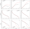Fig. 1 Profile comparison for the 3D averaged models (solid black) by Moens et al. (2022a) for the Γ2, Γ3 and Γ4 WR stars (from left to right) with 1D PoWRHD models using the same basic parameters (dashed-red). Upper panels: wind velocity profiles. Middle panels: density profiles. Lower panels: gas temperature profiles.

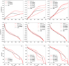Fig. 2 Profile comparison for the Γ2, Γ3, and Γ4 stars. Upper panels: wind velocity profile, in solid black for the 3D averaged model of Moens et al. (2022a), red-dashed lines for the 1D PoWRHD using the same basic parameters, dotted for the PoWRHD changing the mass, dash-dotted for the PoWRHD changing the luminosity value with respect to Moens et al. (2022a), lighter red for the PoWRHD with vDop = 50 km s−1 and boldred for the 1D PoWR approach with a β-law, from left to right for the Γ2, Γ3, and Γ4 WR stars, respectively. Middle panels: same as the upper panel but for the density profile. Lower panel: same as the upper panel but for the gas temperature.

3.1.3 Hydrodynamic 1D models with turbulent pressure, different Doppler velocities, and clumping factors

One parameter that usually plays a more technical role in the calculation of 1D atmosphere models is the Doppler velocity (v_Dop) used in the CMF radiative transfer. In contrast to the spectral synthesis, where this value is usually calculated directly from the thermal and microturbulent broadening, the CMF calculations use a fixed, depth-independent value which not only defines the resolution of the frequency grid, but also enters the Gaussian profiles assumed for the opacity calculations. For WR models, this value is typically set to v_Dop = 100 km s⁻¹, accounting for both thermal and turbulent broadening. While v_Dop as such does not enter the hydrodynamic equation, it indirectly impacts the radiative force calculated in the CMF, in particular in the subsonic regime where a larger value can lead to a slightly higher a_rad values due to a broadening of the otherwise very narrow profiles.

To obtain wind parameters and structure profiles closer to the models from Moens et al. (2022a), we also investigated the effect on changing the Doppler velocities (v_Dop) in the PoWR^HD models. The stellar parameters as well as the profile stratifications are shown in Table 2 and Fig. 2 in light red for the Γ3 and Γ4 models. For the Γ2 representation, the log $\dot{M}$ values dropped below −5.0, where we stopped the calculations as the 3D model yields −4.82. In the Γ2 case, the opacities of the hot iron bump seem to be too low when just assuming v_Dop = 50 km s⁻¹ and our default turbulent velocity of 21 km s⁻¹. For the Γ3 equivalent 1D model, a simple reduction to v_Dop = 50 km s⁻¹ does indeed reduce the discrepancy in $\dot{M}$ obtained; namely, from −4.36 to −4.41, which is still 0.08 dex above the 3D result. Interestingly, v_Dop = 50 km s⁻¹ seems to be a good choice in the Γ4 case, where the reduction from 100 km s⁻¹ to 50 km s⁻¹ changes the mass-loss rate from −4.11 to −4.13, essentially coinciding with the 3D value of −4.14. However, this agreement does not hold for the terminal velocities, although the value of 1630 km s⁻¹ is closer to the 1350 km s⁻¹ result from the 3D simulations.

Our test calculations reveal that there seems to be no fixed value of v_Dop that could generally lead to a better alignment between 1D and 3D results. Interestingly, the different results actually show that higher values of v_Dop are required for models with lower mass-loss rates, further away from the Eddington Limit. Based on a further test calculation with an even lower v_Dop = 20 km s⁻¹ for the Γ3-model, we obtained a scaling for log $\dot{M}$ with log v_Dop: $\frac{\partial \text{log}\dot{M}}{\partial \log v_{\text{Dop}}}\simeq 0.26,$(5) as illustrated in Fig. B.1. We note that both the slope and value differ from the microturbulent velocity scaling found for OB star models by Björklund et al. (2021). For the WR stars, we assumed higher v_Dop values than in the OB star regime since the stellar lines are very broad and a high v_Dop minimizes the computational time with usually no noticeable effect on the spectral synthesis in case of optically thick winds.

All PoWR^HD models presented up to this point include a small turbulent pressure in the hydrodynamic equation with a turbulent velocity of value of 21 km s⁻¹. When comparing to the O supergiant findings by Debnath et al. (2024), this value might be too low; particularly in the regime of the Γ2-model where the lower v_Dop-model did not converge and the opacity increase from the higher v_Dop might indirectly counter the effect of an underestimated turbulent pressure.

To investigate the combined effect of v_Dop and turbulent pressure, we chose to vary the latter component in Eq. (3) by changing v_turb, similarly to González-Torà et al. (2025). Figure 3 shows the log $\dot{M}/M_{\odot }{\text{yr}}^{-1}$, log T_eff, and v_∞ obtained when including different (radially constant) v_turb values ranging from 0 to 106 km s⁻¹ with Δv_turb ∼20 km s⁻¹ for Γ3, assuming a Doppler velocity of v_Dop = 100 km s⁻¹ (light color) and a lower v_Dop = 50 km s⁻¹ (dark color). The velocity, density, and temperature stratifications for the Γ3 PoWR^HD models with different v_turb are shown in Fig. 4 with respect to the averaged 3D profiles for the Γ3 model from Moens et al. (2022a) for v_Dop = 100 km s⁻¹ (light color) and v_Dop = 50 km s⁻¹ (dark color).

As shown in Fig. 4, the default turbulent velocity of 21 km s⁻¹ has a very small effect on the derived wind parameters and, therefore, it cannot explain the higher $\dot{M}$ in comparison to the 3D models. However, when lowering the v_Dop, we obtain overall reduced values of the global stellar parameters and profiles for the same value of v_turb, getting closer to the results from the averaged 3D models.

In addition, we explored the effect of changing the density contrast, D, in the PoWR models. Specifically, D denotes the overdensity factor of the clumps compared to a smooth wind. The formal definitions vary a bit between different atmosphere codes (see Sander et al. 2024, for a recent comparison), but in the limit of optically thin clumping with a void interclump medium (as applied in this work), D is identical to f_cl and the inverse of the volume filling factor. In Fig. 5, we give the output $\text{log\hspace{0.17em}}\dot{M}/M_{\odot }{\text{yr}}^{-1}$, log T_eff, and v_∞ with respect to D for a Γ3 PoWR^HD model with the same stellar parameters as Table 1 and v_Dop = 100 km s⁻¹. The clumping increases from smooth inner with following the clumping law from Hillier et al. (2003) with a characteristic velocity of 100 km s⁻¹. Figure 6 shows the radial velocity, density, and gas temperature stratifications for 1D models with different D parameters with respect to the 3D averaged Γ3 model from Moens et al. (2022a).

The upper panels in Figs. 3 and 5 show that we obtain a higher $\dot{M}/M_{\odot }{\text{yr}}^{-1}$ when increasing the v_turb or D. Even with the lowest assumptions of a smooth model (D = 1) and no turbulent pressure (v_turb = 0 km s⁻¹), we still cannot reach the low $\dot{M}/M_{\odot }{\text{yr}}^{-1}$ values predicted by the 3D models for Γ3. The middle panels in Figs. 3 and 5 show an anti-correlation between increased v_turb or D and lower log T_eff, which is a direct consequence of the corresponding change in $\dot{M}$. In all cases, the T_eff value from Moens et al. (2022a) is again underestimated by ∼30 kK. However, the different calculation methods of T_eff for the multi-D simulations present a high dispersion (e.g., already to the order of ∼kK for O stars). In addition, the different temperature estimation methods between the 1D and 3D methodologies mentioned above (i.e., the 3D models forcing the gas and radiation temperatures to be the same) can also help explain the mismatch between both T_eff values.

The lower panels in Figs. 3 and 5 show the terminal velocity (v_∞). While the effect of increasing the turbulence is small, presenting just a difference of 50 km s⁻¹ for an increase of Δv_turb = 60 km s⁻¹, increasing the density contrast has a strong effect on v_∞ with a difference of almost 500 km s⁻¹ between a smooth model and a clumped model with D = 10. This effect is also visible in the velocity profiles of Figs. 4 and 6, while the density and temperature profiles do not present significant v_turb or D dependency.

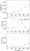Fig. 3 Different PoWRHD models for Γ3 with vDop = 100 km s−1 (light color) and vDop = 50 km s−1 (dark color) including a turbulence vturb with respect to the $\dot{M}/M_{\odot }{\text{yr}}^{-1}$, log Teff, and v∞.

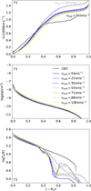Fig. 4 Radial velocity, density and gas temperature profiles for the averaged 3D model from Moens et al. (2022a) in solid black and PoWRHD models for Γ3 vDop = 100 km s−1 (light color) and vDop = 50 km s−1 (dark color) including different turbulence values, vturb.

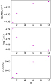Fig. 5 Different PoWRHD models for Γ3 including a turbulence vturb = 21 km s−1 with respect to the $\log \dot{M}/M_{\odot }{\text{yr}}^{-1}$, log Teff, and v∞.

3.1.4 1D β-law models

Figure 2 also shows the wind velocity, density and gas temperature profiles from the β-law PoWR approach using the solution of the hydrostatic equation in the (quasi)hydrostatic regime and a β-law (Eq. (1)) for the supersonic wind regime, commonly adopting β = 1.0 for WR stars (Hillier 1988; Hamann et al. 1988; Hillier & Miller 1999), shown in solid red. Table 2 shows the final parameters for the β-law approach with the same R_⋆, log(L_⋆/L_⊙), M_⋆/M_⊙, v_∞, and log $\dot{M}$ as Moens et al. (2022a) for the Γ2, Γ3, and Γ4 models, respectively.

The main difference between the β-law and the hydrodynamically consistent 1D modeling approaches illustrated in Fig. 2 is the wind velocity in the outer layers: while the hydrodynamical solution shows a flattening or even deceleration at 1 −R_c/r ∼0.45, the β-law approach has a continuing velocity increase and cannot account for any deceleration in the velocity due to the dense medium in the outer layers of WR stars. Hence, it predicts an unrealistic profile, which will not change even if v_∞ was adjusted to the 3D results. Specifically, for the Γ4-model, the β-law model starts already in the supersonic regime with a nonzero radial velocity. The β-law model still give a reasonable reproduction of the general density structure (cf. middle panels in Fig. 2), although considerable deviations are also noticeable for the inner part of the Γ4-model. The temperature profiles show the usual deviations in the outer wind regime with the β-law model being significantly hotter in the inner wind. However, as we discuss in Sect. 3.2, the different temperature profiles do not significantly affect the resulting spectral line predictions.

Fig. 6 Radial velocity, density and gas temperature profiles for the averaged 3D model from Moens et al. (2022a) in solid black and PoWRHD models for Γ3 including different turbulence values, vturb.

3.2 Spectral synthesis for PoWR models

To study the implications of the stratifications predicted by the 3D calculations from Moens et al. (2022a), we compared the resulting synthetic spectra from the different 1D PoWR approaches. Figures 7 and 8 show the computed UV and optical spectra for the β-law PoWR framework (solid blue) and the different PoWR^HD approaches: the initial models with fixed stellar mass and luminosity (dashed red), the model with flexible stellar mass (dotted black), and with flexible luminosity (dash-dotted green) for the Γ2, Γ3, and Γ4 models, respectively. We also include in the legend the so-called transformed mass loss rate, ${\dot{M}}_{\text{t}}$, defined as:

${\dot{M}}_{\text{t}}=\dot{M}\sqrt{D}\left(\frac{1000\text{km\hspace{0.17em}s}{}^{-1}}{{\nu }_{\infty }}\right){\left(\frac{{10}^6{L}_{\odot }}{L}\right)}^{3/4}.$(6)

This quantity was introduced by Gräfener & Vink (2013) and refers to the inferred mass-loss rate the star would have with a D = 1, luminosity of 10⁶ L_⊙, and v_∞ = 1000 km s⁻¹. Similarly to the context of the “transformed radius” (Schmutz et al. 1989), stars with a similar ${\dot{M}}_{\text{t}}$ are expected to display a similar spectrum. A look at Figs. 7 and 8 confirms that this is indeed the case. A zoomed-in version for the UV spectra is shown in Figure C.1.

In the case of Γ2, the main difference between β-law and PoWR^HD models is in the N V 4604 Å and N III 4640 Å optical lines. This is due to the different ionization states for the β-law and hydrodynamical models: in the outer layers of the hydrodynamical models the He III has recombined to He II, as well as N V to N IV. This is not the case for the β-law model. For Γ3, both the UV and optical present overall higher emission lines for the initial PoWR^HD model. This difference can be explained with the log $\dot{M}/M_{\odot }{\text{yr}}^{-1}=-4.36$, which is 0.15 dex higher for the PoWR^HD model when compared to all the other approaches. For Γ4, all model approaches present a very similar UV and optical spectra, with very close agreement between the stellar parameters in Table 2.

Figures 9 and 10 show the UV and optical spectral regions for the PoWR^HD with fixed stellar mass, luminosity, and v_Dop = 50 km s⁻¹, but varying turbulence. A zoomed-in version for the UV spectra is shown in Figure C.2. We see that unlike for the O stars in González-Torà et al. (2025), the change in turbulence does not significantly affect the spectral lines, as the impact concerns the broadening of lines in the quasihydrostatic regime; whereas here, all the lines are formed in the wind.

Figures 11 and 12 show the UV and optical synthetic spectra from the models with different density contrasts, from a smooth model with D = 1 to a clumped model with D = 10, following the clumping law from Hillier et al. (2003) and a characteristic velocity of 100 km s⁻¹. A zoomed-in version for the UV spectra is shown in Figure C.3. While the UV spectra remain relatively unchanged, the optical spectra present a difference in N V 4604 Å and N III 4640 Å and to a lesser extent the N IV 4057 Å line because of the high terminal velocities in the outer wind.

Despite the slight changes on the optical spectra in Figs. 8 and 12, the optical regime does not fully reflect the differences in wind characteristics and can ultimately be prone to degeneracies in parameter determination. In this case, as pointed out by Lefever et al. (2023), the UV yield much better diagnostics as the extent of wind differences is only fully reflected in well-resolved P-Cygni lines such as C IV 1550 Å. To illustrate the wind differences, Figures D.1, D.2, and D.3 present a zoom-in on the UV C IV 1550 Å line, corresponding to the models shown in Figs. 7, 9, and 11, respectively. In Fig. D.1, for all the Γ2, Γ3, and Γ4 profiles, the blue-most part of the absorption troughs shift significantly in accordance with wind parameter differences of the various models (see, e.g., v_∞ in Table 2). In Fig. D.3, the different clumping parameters will also affect the P Cygni line, as expected. In contrast, there is very little variation in the P Cygni line in Fig. D.2, which illustrates the changes in v_turb. This little variation is expected with the comparatively minor wind changes in Figs. 3 and 4.

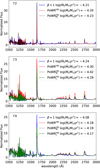Fig. 7 Computed UV spectra for the PoWR models. From top to bottom: β-law approach (blue solid line), the PoWRHD with identical input as Moens et al. (2022a) (red dashed-dotted), the PoWRHD with flexible mass (black dotted line), and the PoWRHD with flexible luminosity (green dash-dotted line), for Γ2, Γ3, and Γ4 models, respectively.

Fig. 8 Same as Fig. 7, but for the optical spectral region.

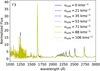Fig. 9 Computed UV spectra for the PoWRHD Γ3 models, including different vturb values.

Fig. 10 Same as Fig. 9, for the optical spectral range.

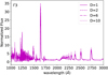Fig. 11 Computed UV spectra for the PoWRHD Γ3 models, including different density contrast values.

Fig. 12 Same as Fig. 11, but for the optical spectral range.

4 Conclusions

In this work, we compare two different complementary hydrodynamical modeling approaches to reproduce the atmospheric layers and stellar outflows of three cWR stars: 1) the 1D, spherically symmetric, stationary and non-LTE PoWR^HD framework and 2) the 3D, box-in-a-star, time-evolution, LTE models from Moens et al. (2022a). While necessary, it is currently computationally unfeasible for atmospheric models to solve the complex interplay between radiation field and atomic physics with 3D and time-dependent simulations. Therefore, using and comparing these two complementary modeling approaches is paramount to retrieving valuable knowledge on the atmospheres of WRs.

Generally, we obtained a very good agreement between the two methods. The 1D models managed to reproduce the overall behavior of the averaged velocity, density, and temperature stratification of the 3D models. We find that the density is best reproduced when the velocities are only slightly overestimated and temperatures in the outer wind are lower in 1D models, which is similar to our O-star comparison and likely a consequence of the different treatments (see also González-Torà et al. 2025). For the same stellar masses and luminosities as in Moens et al. (2022a), the 1D PoWR^HD models overestimate log $\dot{M}$ by up to ≲0.2 dex and v (6 R_*) by up to ∼400 km s⁻¹. Consequently, the resulting effective temperatures are lower by 0.2 dex (∼30 kK).

These discrepancies can largely be mitigated by small adjustments of the mass (<2%) or the luminosity (<0.1 dex) of the 1D models. Such differences are in agreement with the mass loss and luminosity dispersions obtained by the 3D simulations.

We further explored the effect on varying additional parameters inherent to hydrodynamically consistent 1D PoWR^HD models, namely clumping, Doppler velocity, and turbulent pressure, and compared with a β-law model. Clumping usually worsens the agreement with the 3D average velocity, which is expected given the low clumping amount in the Moens et al. (2022a) models. Decreasing the Doppler velocity in the PoWR models from 100 km s⁻¹ to 50 km s⁻¹ can help reconcile the discrepancies between both 1D and 3D approaches, but the necessary Doppler velocity seems to be regime-dependent with models further away from the Eddington limit requiring a higher Doppler velocity. The inclusion of a larger, constant turbulent pressure in the models slightly increases the derived mass-loss rates and also the terminal velocities.

Using the ability of PoWR to perform spectral synthesis, we compared the resulting model spectra of the different 1D PoWR^HD representations and a β-law model, adopting the main 3D model parameters. While the β-law branch overall matches the PoWR^HD spectra for the optical part, notable differences are seen for the N V 4604 Å and N III 4640 Å lines due to the different ionization states between the Γ2 PoWR^HD and the β-law approaches.

The Γ2, Γ3, and Γ4 models reproduced here assume a wind launched in the subsurface regions of a supersonic optically thick regime and this is aptly reproduced by the 1D PoWR models. This consistency enables us to take a reasonable approach to performing a spectral analysis of cWR stars with dynamically consistent models in future works. Nonetheless, our models have problems with the lower luminosity Γ1 model in Moens et al. (2022a), simulating an inflated and turbulent atmosphere with an optically thin line-driven wind on top, which corresponds more to a transition from a WR to a stripped hot (sub)dwarf. We could not obtain a converged model for the Γ1 model with the current version of PoWR^HD, obtaining unrealistically low $\dot{M}$ values. This is likely the result of the current inability to reproduce the turbulent environment with a subsequent wind launching. Further updates of the hydrodynamic treatment in 1D atmospheres, such as an improved, depth-dependent treatment of turbulent pressure, could help bridge the regime between hot stripped stars and cWR stars.

Acknowledgements

GGT is supported by the German Deutsche Forschungs-gemeinschaft (DFG) under Project-ID 496854903 (SA4064/2-1, PI Sander). GGT further acknowledges financial support by the Federal Ministry for Economic Affairs and Climate Action (BMWK) via the German Aerospace Center (Deutsches Zentrum für Luftund Raumfahrt, DLR) grant 50 OR 2503 (PI: Sander). AS, MBP, RRL, and JJ are supported by the German Deutsche Forschungsgemeinschaft (DFG) under Project-ID 445674056 (Emmy Noether Research Group SA4064/1-1, PI Sander). GGT and AS further acknowledge support from the Federal Ministry of Education and Research (BMBF) and the Baden-Württemberg Ministry of Science as part of the Excellence Strategy of the German Federal and State Governments. JOS, DD, LD, NM, CVdS acknowledge the support of the European Research Council (ERC) Horizon Europe grant under grant agreement number 101044048 (ERC-2021-COG, SUPERSTARS-3D) and from KU Leuven C1 grant BRAVE C16/23/009. OV, JOS, and LD acknowledge the support of the Belgian Research Foundation Flanders (FWO) Odysseus program under grant number G0H9218N and FWO grant G077822N.

Appendix A Gas, radiative and flux temperatures

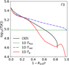Fig. A.1 Flux temperature (dashed green line) and radiation temperature (dashed blue line) for the Γ3 model obtained from the total emergent flux, compared to the gas temperature stratifications for the averaged ⟨3D⟩ model.

Appendix B $\text{log\hspace{0.17em}}\dot{M}$ vs log v_Dop scaling

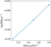Fig. B.1 Obtained log $\dot{M}$ with respect to the assumed log vDop for the Γ3 models.

Appendix C Zoomed-in UV spectra

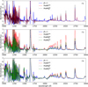Fig. C.1 Zoomed-in of the computed UV spectra for the PoWR models. From up to down: the β-law approach (blue solid line), the PoWRHD with identical input as Moens et al. (2022a) (red dashed dotted), the PoWRHD with flexible mass (black dotted line) and the PoWRHD with flexible luminosity (green dash-dotted line), for Γ2, Γ3 and Γ4 models, respectively.

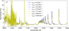Fig. C.2 Zoom-in on the computed UV spectra for the PoWRHD Γ3 models, including different vturb values.

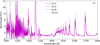Fig. C.3 Zoom-in on the computed UV spectra for the PoWRHD Γ3 models, including different density contrast values.

Appendix D The UV C IV − 1550 Å P-Cygni profile

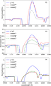Fig. D.1 UV C IV 1550 Å P-Cygni profile for the PoWR models. From top to bottom: β-law approach (blue solid line), the PoWRHD with identical input as Moens et al. (2022a) (red dashed dotted), the PoWRHD with flexible mass (black dotted line) and the PoWRHD with flexible luminosity (green dash-dotted line), for Γ2, Γ3 and Γ4 models, respectively.

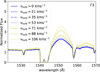Fig. D.2 UV C IV − 1550 Å P-Cygni profile for the PoWRHD Γ3 models, including a different vturb values.

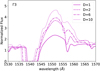Fig. D.3 UV C IV − 1550 Å P-Cygni profile for the PoWRHD Γ3 models, including a different density contrast values.

References

All Tables

All Figures

	Fig. 1 Profile comparison for the 3D averaged models (solid black) by Moens et al. (2022a) for the Γ2, Γ3 and Γ4 WR stars (from left to right) with 1D PoWRHD models using the same basic parameters (dashed-red). Upper panels: wind velocity profiles. Middle panels: density profiles. Lower panels: gas temperature profiles.
In the text

Fig. 2 Profile comparison for the Γ2, Γ3, and Γ4 stars. Upper panels: wind velocity profile, in solid black for the 3D averaged model of Moens et al. (2022a), red-dashed lines for the 1D PoWRHD using the same basic parameters, dotted for the PoWRHD changing the mass, dash-dotted for the PoWRHD changing the luminosity value with respect to Moens et al. (2022a), lighter red for the PoWRHD with vDop = 50 km s−1 and boldred for the 1D PoWR approach with a β-law, from left to right for the Γ2, Γ3, and Γ4 WR stars, respectively. Middle panels: same as the upper panel but for the density profile. Lower panel: same as the upper panel but for the gas temperature.

In the text

	Fig. 3 Different PoWRHD models for Γ3 with vDop = 100 km s−1 (light color) and vDop = 50 km s−1 (dark color) including a turbulence vturb with respect to the $\dot{M}/M_{\odot }{\text{yr}}^{-1}$, log Teff, and v∞.
In the text

	Fig. 4 Radial velocity, density and gas temperature profiles for the averaged 3D model from Moens et al. (2022a) in solid black and PoWRHD models for Γ3 vDop = 100 km s−1 (light color) and vDop = 50 km s−1 (dark color) including different turbulence values, vturb.
In the text

	Fig. 5 Different PoWRHD models for Γ3 including a turbulence vturb = 21 km s−1 with respect to the $\log \dot{M}/M_{\odot }{\text{yr}}^{-1}$, log Teff, and v∞.
In the text

	Fig. 6 Radial velocity, density and gas temperature profiles for the averaged 3D model from Moens et al. (2022a) in solid black and PoWRHD models for Γ3 including different turbulence values, vturb.
In the text

	Fig. 7 Computed UV spectra for the PoWR models. From top to bottom: β-law approach (blue solid line), the PoWRHD with identical input as Moens et al. (2022a) (red dashed-dotted), the PoWRHD with flexible mass (black dotted line), and the PoWRHD with flexible luminosity (green dash-dotted line), for Γ2, Γ3, and Γ4 models, respectively.
In the text

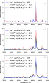	Fig. 8 Same as Fig. 7, but for the optical spectral region.
In the text

	Fig. 9 Computed UV spectra for the PoWRHD Γ3 models, including different vturb values.
In the text

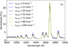	Fig. 10 Same as Fig. 9, for the optical spectral range.
In the text

	Fig. 11 Computed UV spectra for the PoWRHD Γ3 models, including different density contrast values.
In the text

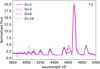	Fig. 12 Same as Fig. 11, but for the optical spectral range.
In the text

	Fig. A.1 Flux temperature (dashed green line) and radiation temperature (dashed blue line) for the Γ3 model obtained from the total emergent flux, compared to the gas temperature stratifications for the averaged ⟨3D⟩ model.
In the text

	Fig. B.1 Obtained log $\dot{M}$ with respect to the assumed log vDop for the Γ3 models.
In the text

	Fig. C.1 Zoomed-in of the computed UV spectra for the PoWR models. From up to down: the β-law approach (blue solid line), the PoWRHD with identical input as Moens et al. (2022a) (red dashed dotted), the PoWRHD with flexible mass (black dotted line) and the PoWRHD with flexible luminosity (green dash-dotted line), for Γ2, Γ3 and Γ4 models, respectively.
In the text

	Fig. C.2 Zoom-in on the computed UV spectra for the PoWRHD Γ3 models, including different vturb values.
In the text

	Fig. C.3 Zoom-in on the computed UV spectra for the PoWRHD Γ3 models, including different density contrast values.
In the text

	Fig. D.1 UV C IV 1550 Å P-Cygni profile for the PoWR models. From top to bottom: β-law approach (blue solid line), the PoWRHD with identical input as Moens et al. (2022a) (red dashed dotted), the PoWRHD with flexible mass (black dotted line) and the PoWRHD with flexible luminosity (green dash-dotted line), for Γ2, Γ3 and Γ4 models, respectively.
In the text

	Fig. D.2 UV C IV − 1550 Å P-Cygni profile for the PoWRHD Γ3 models, including a different vturb values.
In the text

	Fig. D.3 UV C IV − 1550 Å P-Cygni profile for the PoWRHD Γ3 models, including a different density contrast values.
In the text

References

- Abbott, D. C., & Conti, P. S. 1987, ARA&A, 25, 113 [NASA ADS] [CrossRef] [Google Scholar]
- Asplund, M., Grevesse, N., Sauval, A. J., & Scott, P. 2009, ARA&A, 47, 481 [NASA ADS] [CrossRef] [Google Scholar]
- Björklund, R., Sundqvist, J. O., Puls, J., & Najarro, F. 2021, A&A, 648, A36 [EDP Sciences] [Google Scholar]
- Castor, J. I., Abbott, D. C., & Klein, R. I. 1975, ApJ, 195, 157 [Google Scholar]
- Conti, P. S. 1975, Mem. Soc. Roy. Sci. Liege, 9, 193 [Google Scholar]
- Debnath, D., Sundqvist, J. O., Moens, N., et al. 2024, A&A, 684, A177 [NASA ADS] [CrossRef] [EDP Sciences] [Google Scholar]
- de Koter, A., Heap, S. R., & Hubeny, I. 1997, ApJ, 477, 792 [Google Scholar]
- Dsilva, K., Shenar, T., Sana, H., & Marchant, P. 2020, A&A, 641, A26 [NASA ADS] [CrossRef] [EDP Sciences] [Google Scholar]
- Gayley, K. G. 1995, ApJ, 454, 410 [Google Scholar]
- González-Torà, G., Sander, A. A. C., Sundqvist, J. O., et al. 2025, A&A, 694, A269 [NASA ADS] [CrossRef] [EDP Sciences] [Google Scholar]
- Gräfener, G., & Hamann, W. R. 2005, A&A, 432, 633 [NASA ADS] [CrossRef] [EDP Sciences] [Google Scholar]
- Gräfener, G., & Hamann, W. R. 2008, A&A, 482, 945 [Google Scholar]
- Gräfener, G., & Vink, J. S. 2013, A&A, 560, A6 [NASA ADS] [CrossRef] [EDP Sciences] [Google Scholar]
- Gräfener, G., Koesterke, L., & Hamann, W. R. 2002, A&A, 387, 244 [NASA ADS] [CrossRef] [EDP Sciences] [Google Scholar]
- Gräfener, G., Owocki, S. P., & Vink, J. S. 2012, A&A, 538, A40 [NASA ADS] [CrossRef] [EDP Sciences] [Google Scholar]
- Grevesse, N., & Noels, A. 1993, in Origin and Evolution of the Elements, eds. N. Prantzos, E. Vangioni-Flam, & M. Casse, 15 [Google Scholar]
- Hamann, W. R. 1986, A&A, 160, 347 [NASA ADS] [Google Scholar]
- Hamann, W. R., & Gräfener, G. 2003, A&A, 410, 993 [CrossRef] [EDP Sciences] [Google Scholar]
- Hamann, W. R., & Gräfener, G. 2004, A&A, 427, 697 [NASA ADS] [CrossRef] [EDP Sciences] [Google Scholar]
- Hamann, W. R., & Koesterke, L. 1998, A&A, 335, 1003 [Google Scholar]
- Hamann, W. R., Schmutz, W., & Wessolowski, U. 1988, A&A, 194, 190 [Google Scholar]
- Hamann, W. R., Gräfener, G., & Liermann, A. 2006, A&A, 457, 1015 [NASA ADS] [CrossRef] [EDP Sciences] [Google Scholar]
- Hamann, W. R., Gräfener, G., Oskinova, L., & Liermann, A. 2008, in Mass Loss from Stars and the Evolution of Stellar Clusters, eds. A. de Koter, L. J. Smith, & L. B. F. M. Waters, Astronomical Society of the Pacific Conference Series, 388, 171 [Google Scholar]
- Hillier, D. J. 1988, ApJ, 327, 822 [Google Scholar]
- Hillier, D. J. 2003, in Stellar Atmosphere Modeling, eds. I. Hubeny, D. Mihalas, & K. Werner, Astronomical Society of the Pacific Conference Series, 288, 199 [NASA ADS] [Google Scholar]
- Hillier, D. J., & Miller, D. L. 1998, ApJ, 496, 407 [NASA ADS] [CrossRef] [Google Scholar]
- Hillier, D. J., & Miller, D. L. 1999, ApJ, 519, 354 [Google Scholar]
- Hillier, D. J., Lanz, T., Heap, S. R., et al. 2003, ApJ, 588, 1039 [Google Scholar]
- Hubeny, I., & Lanz, T. 2003, in Stellar Atmosphere Modeling, eds. I. Hubeny, D. Mihalas, & K. Werner, Astronomical Society of the Pacific Conference Series, 288, 51 [NASA ADS] [Google Scholar]
- Iglesias, C. A., & Rogers, F. J. 1996, ApJ, 464, 943 [NASA ADS] [CrossRef] [Google Scholar]
- Kubát, J., Puls, J., & Pauldrach, A. W. A. 1999, A&A, 341, 587 [NASA ADS] [Google Scholar]
- Lefever, R. R., Sander, A. A. C., Shenar, T., et al. 2023, MNRAS, 521, 1374 [NASA ADS] [CrossRef] [Google Scholar]
- Moens, N., Poniatowski, L. G., Hennicker, L., et al. 2022a, A&A, 665, A42 [NASA ADS] [CrossRef] [EDP Sciences] [Google Scholar]
- Moens, N., Sundqvist, J. O., El Mellah, I., et al. 2022b, A&A, 657, A81 [NASA ADS] [CrossRef] [EDP Sciences] [Google Scholar]
- Moffat, A. F. J. 2015, in Wolf–Rayet Stars, eds. W.-R. Hamann, A. Sander, & H. Todt, 13 [Google Scholar]
- Nugis, T., & Lamers, H. J. G. L. M. 2002, A&A, 389, 162 [EDP Sciences] [Google Scholar]
- Paczyński, B. 1967, Acta Astron., 17, 355 [NASA ADS] [Google Scholar]
- Pauldrach, A., Puls, J., & Kudritzki, R. P. 1986, A&A, 164, 86 [NASA ADS] [Google Scholar]
- Poniatowski, L. G., Sundqvist, J. O., Kee, N. D., et al. 2021, A&A, 647, A151 [NASA ADS] [CrossRef] [EDP Sciences] [Google Scholar]
- Poniatowski, L. G., Kee, N. D., Sundqvist, J. O., et al. 2022, A&A, 667, A113 [NASA ADS] [CrossRef] [EDP Sciences] [Google Scholar]
- Portinari, L., Chiosi, C., & Bressan, A. 1998, A&A, 334, 505 [NASA ADS] [Google Scholar]
- Puls, J. 2008, in Massive Stars as Cosmic Engines, 250, eds. F. Bresolin, P. A. Crowther, & J. Puls, 25 [NASA ADS] [Google Scholar]
- Puls, J., Urbaneja, M. A., Venero, R., et al. 2005, A&A, 435, 669 [NASA ADS] [CrossRef] [EDP Sciences] [Google Scholar]
- Richardson, N. D., Lee, L., Schaefer, G., et al. 2021, ApJ, 908, L3 [NASA ADS] [CrossRef] [Google Scholar]
- Sander, A. A. C. 2015, PhD thesis, University of Potsdam, Germany [Google Scholar]
- Sander, A. A. C. 2017, in The Lives and Death-Throes of Massive Stars, 329, eds. J. J. Eldridge, J. C. Bray, L. A. S. McClelland, & L. Xiao, 215 [NASA ADS] [Google Scholar]
- Sander, A. A. C., & Vink, J. S. 2020, MNRAS, 499, 873 [Google Scholar]
- Sander, A., Todt, H., Hainich, R., & Hamann, W. R. 2014, A&A, 563, A89 [NASA ADS] [CrossRef] [EDP Sciences] [Google Scholar]
- Sander, A., Shenar, T., Hainich, R., et al. 2015, A&A, 577, A13 [NASA ADS] [CrossRef] [EDP Sciences] [Google Scholar]
- Sander, A. A. C., Hamann, W. R., Todt, H., Hainich, R., & Shenar, T. 2017, A&A, 603, A86 [NASA ADS] [CrossRef] [EDP Sciences] [Google Scholar]
- Sander, A. A. C., Vink, J. S., & Hamann, W. R. 2020, MNRAS, 491, 4406 [Google Scholar]
- Sander, A. A. C., Lefever, R. R., Poniatowski, L. G., et al. 2023, A&A, 670, A83 [NASA ADS] [CrossRef] [EDP Sciences] [Google Scholar]
- Sander, A. A. C., Bouret, J. C., Bernini-Peron, M., et al. 2024, A&A, 689, A30 [NASA ADS] [CrossRef] [EDP Sciences] [Google Scholar]
- Schmutz, W., Hamann, W. R., & Wessolowski, U. 1989, A&A, 210, 236 [Google Scholar]
- Shenar, T. 2024, arXiv e-prints [arXiv:2410.04436] [Google Scholar]
- Shenar, T., Bodensteiner, J., Abdul-Masih, M., et al. 2020, A&A, 639, L6 [EDP Sciences] [Google Scholar]
- Smith, N. 2014, ARA&A, 52, 487 [NASA ADS] [CrossRef] [Google Scholar]
- Smith, N., & Conti, P. S. 2008, ApJ, 679, 1467 [NASA ADS] [CrossRef] [Google Scholar]
- Sundqvist, J. O., Owocki, S. P., & Puls, J. 2018, A&A, 611, A17 [NASA ADS] [CrossRef] [EDP Sciences] [Google Scholar]
- ud-Doula, A., Sundqvist, J. O., Narechania, N., et al. 2025, A&A, 693, A224 [NASA ADS] [CrossRef] [EDP Sciences] [Google Scholar]
- van der Hucht, K. A., Conti, P. S., Lundstrom, I., & Stenholm, B. 1981, Space Sci. Rev., 28, 227 [Google Scholar]
- Wolf, C. J. E., & Rayet, G. 1867, Acad. Sci. Paris Comptes Rendus, 65, 292 [Google Scholar]
- Xia, C., Teunissen, J., El Mellah, I., Chané, E., & Keppens, R. 2018, ApJS, 234, 30 [Google Scholar]
Historically, the term “classical WR” was used for all Population I WR stars (e.g., van der Hucht et al. 1981). This slowly changed after the discovery of hydrogen-burning very massive stars with WR-type spectral features (e.g., de Koter et al. 1997; Smith & Conti 2008).
This does not apply for the crucial (average) wind launching region around the sonic point (Sander et al. 2017; González-Torà et al. 2025).
Additionally, the 3D averaged velocity profiles show an nonphysical spike at the lower boundary, this is due to numerical problems in the boundary conditions of the multidimensional simulations.
All Tables
Comparison of the resulting wind parameters and effective temperatures predicted by the 1D PoWRHD and the 3D RHD models from Moens et al. (2022a, denoted as M+22) when using the same basic input parameters.
Stellar parameters for the β-law and modified hydrodynamical PoWR models to match the profile of Moens et al. (2022a).