| Issue |
A&A
Volume 694, February 2025
|
|
|---|---|---|
| Article Number | A326 | |
| Number of page(s) | 9 | |
| Section | Numerical methods and codes | |
| DOI | https://doi.org/10.1051/0004-6361/202451786 | |
| Published online | 25 February 2025 | |
Disentangling stellar atmospheric parameters in astronomical spectra using generative adversarial neural networks
Application to Gaia/RVS parameterisation
1
Universidade da Coruña (UDC), Department of Nautical Sciences and Marine Engineering,
Paseo de Ronda 51,
15011 A
Coruña,
Spain
2
CIGUS CITIC, Centre for Information and Communications Technologies Research, Universidade da Coruña,
Campus de Elviña s/n,
15071 A
Coruña,
Spain
3
Universidade da Coruña (UDC), Department of Computer Science and Information Technologies,
Campus Elviña s/n,
15071 A
Coruña,
Spain
4
Universidad de Guadalajara, Instituto de Astronomía y Meteorología,
Jalisco,
Mexico
★ Corresponding author; This email address is being protected from spambots. You need JavaScript enabled to view it.
Received:
3
August
2024
Accepted:
18
January
2025
Abstract
Context. The rapid expansion of large-scale spectroscopic surveys has highlighted the need to use automatic methods to extract information about the properties of stars with the greatest efficiency and accuracy, and also to optimise the use of computational resources.
Aims. We developed a method based on generative adversarial networks (GANs) to disentangle the physical (effective temperature and gravity) and chemical (metallicity and overabundance of α elements with respect to iron) atmospheric properties in astronomical spectra. Using a projection of the stellar spectra, commonly called latent space, in which the contribution due to one or several main stellar physicochemical properties is minimised while others are enhanced, it was possible to maximise the information related to certain properties. This could then be extracted using artificial neural networks (ANNs) as regressors, with a higher accuracy than a reference method based on the use of ANNs that had been trained with the original spectra.
Methods. Our model utilises auto-encoders, comprising two ANNs: an encoder and a decoder that transform input data into a low-dimensional representation known as latent space. It also uses discriminators, which are additional neural networks aimed at transforming the traditional auto-encoder training into an adversarial approach. This is done to reinforce the astrophysical parameters or disentangle them from the latent space. We describe our Generative Adversarial Networks for Disentangling and Learning Framework (GANDALF) tool in this article. It was developed to define, train, and test our GAN model with a web framework to show visually how the disentangling algorithm works. It is open to the community in Github.
Results. We demonstrate the performance of our approach for retrieving atmospheric stellar properties from spectra using Gaia Radial Velocity Spectrograph (RVS) data from DR3. We used a data-driven perspective and obtained very competitive values, all within the literature errors, and with the advantage of an important dimensionality reduction of the data to be processed.
Key words: methods: data analysis / techniques: spectroscopic / stars: evolution / stars: fundamental parameters / stars: general / Galaxy: stellar content
© The Authors 2025
 Open Access article, published by EDP Sciences, under the terms of the Creative Commons Attribution License (https://creativecommons.org/licenses/by/4.0), which permits unrestricted use, distribution, and reproduction in any medium, provided the original work is properly cited.
This article is published in open access under the Subscribe to Open model. This email address is being protected from spambots. You need JavaScript enabled to view it. to support open access publication.
1 Introduction
The huge development of massive spectroscopic surveys in recent decades has highlighted the convenience of addressing their exploitation through automatic techniques, often supported by machine learning (ML) methods. ML has become indispensable in astronomy, enabling researchers to handle the vast amounts of data generated by modern telescopes and surveys. Among the examples available in the literature, we can highlight several applications in various fields. In the area of spectroscopic classification, the use of neural networks and support vector machines two decades ago significantly improved the accuracy and efficiency of classifying stars, galaxies, and quasars based on their spectral features. Examples can be found in the pioneering works by Bailer-Jones et al. (1998) and Re Fiorentin et al. (2007) based on the Sloan Digital Sky Survey (SDSS, Abazajian et al. 2009). More recent works, such as those focused on the Gaia survey (Gaia Collaboration 2016), used Gaussian mixture models and decision trees, as done by Hughes et al. (2022) and Delchambre et al. (2023).
In the problem of classification outlier analysis, selfsupervised learning techniques such as auto-encoders and clustering methods such as self-organised maps have been used to detect unusual spectral signatures, which can indicate unique or previously unknown astronomical objects (Baron & Poznanski 2017; Dafonte et al. 2018). ML has also been used to detect exoplanets in light curves from missions such as Kepler (Barbara et al. 2022) and Transiting Exoplanet Survey Satellite (TESS) (Tardugno Poleo et al. 2024). Deep learning models, such as convolutional neural networks (CNNs), have been particularly successful in identifying the subtle dips in brightness that indicate a planet transiting its host star (Shallue & Vanderburg 2018) or, more recently, in detecting hidden molecular signatures in cross-correlated spectra from exoplanetary targets (Garvin et al. 2024).
One of the most effective ML methods for improving knowledge extraction from large datasets is the use of representation learning (RL) algorithms. RL can transform a high-dimensional input vector into a lower-dimensional vector representation. After suitable training, these representations enable models such as t-distributed stochastic neighbour embedding (t-SNE) or Uniform Manifold Approximation and Projection (UMAP) to identify patterns or anomalies within the data. While RL is a broad concept that encompasses all techniques to learn meaningful data representations, disentangled representation is a learning approach in which ML models are designed to acquire representations that can identify and separate the underlying factors embedded in the observed data. Disentangled representation learning (DRL) helps to produce explainable representations of the data, where each component has a clear semantic meaning (Bengio et al. 2013; Lake et al. 2017).
One approach in RL is generative modelling (Bishop 2006), which also consists of a self-supervised learning model that constructs a vector representation of the input data. As a result, the model can be used to generate new data from the learned distribution. In particular, generative adversarial networks (GANs, Goodfellow et al. 2014) address the problem with two submodels: the generator model, which is trained to generate new examples, and the discriminator model, which tries to classify the examples as real (from the domain) or synthetic (generated). The two models are trained simultaneously in a zero-sum adversarial setting, where the generator aims to produce increasingly realistic samples while the discriminator seeks to distinguish between real and synthetic data. Training continues until the discriminator is unable to reliably differentiate between the two, which indicates that the generator is producing plausible examples. In a generative configuration, the adversarial discriminator can be used to assess the quality of a reconstructed signal for which conditioning factors do not exist in the training set (Mathieu et al. 2016; Szabó et al. 2017; Chen et al. 2016). Another alternative, suggested by Fader networks (Lample et al. 2018), is to apply the adversarial discriminator on the latent space itself, which prevents it from containing any information about the specified conditioning factor.
There is abundant literature on separating distinct, independent factors or components of information within a complex dataset or representation. This process has been called information disentangling. In the context of ML, disentangling aims to isolate meaningful, interpretable features such as specific physical parameters or latent factors so they are not entangled with other, unrelated information. GANs can play a significant role in information disentangling by learning to generate complex data distributions while isolating meaningful, interpretable features within the data. They have been used in many domains, typically involving image treatment or reconstruction. For instance, Rifai et al. (2012) applied generative convolutional networks to facial expression recognition, Cheung et al. (2015) used auto-encoders and a cross-covariance penalty to recognise handwritten style, and Chen et al. (2016) applied GANs to several image recognition problems. A recent study by Wang et al. (2024) comprehensively reviews the current state of the literature and provides an in-depth discussion of various methodologies, metrics, models, and applications.
In the astrophysical domain, the problem of disentangling the stellar atmospheric parameter (Teff, logɡ, and the distribution of [M/H] and [α/Fe]) applied to the stellar spectra was first studied by Price-Jones & Bovy (2019), who fitted a polynomial model of the non-chemical parameters (Teff and logɡ) to synthetic spectra in a grid and then used principal component analysis and a clustering algorithm to identify chemically similar groups. Disentangling using neural networks has been recently addressed in de Mijolla et al. (2021) and de Mijolla & Ness (2022). In de Mijolla et al. (2021), a neural network with a supervised disentanglement loss term was applied to a synthetic APOGEE-like dataset of spectra to find chemically identical stars without the explicit use of measured abundances. In a more recent work, Santoveña et al. (2024) (Paper 1) developed a method, also based on GANs, for disentangling the physical (effective temperature and gravity) and chemical (metallicity, overabundance of α elements, and individual elementary abundances) properties of stars in astronomical spectra. In this case, an original version of adversarial training was developed that included the innovation of using one discriminator per stellar parameter to be disentangled. The methodology was demonstrated using APOGEE and Gaia Radial Velocity Spectrograph (RVS) synthetic spectra.
In this article, we explore the use of GANs to extract stellar atmospheric parameters from observational stellar spectra and attain a higher precision in the derived values and a higher computational efficiency than the reference method based on the use of Artificial Neural Networks (ANNs) trained with the spectra. Additionally, we make our Generative Adversarial Networks for Disentangling and Learning Framework (GANDALF) tool available to the astrophysical community. We developed this tool to define, train, and test our GAN model using a web framework to show how the disentangling algorithm works. The paper is structured as follows. Section 2 describes the specific deep-learning architecture of our algorithm, which uses multi-discriminators. We also briefly introduce GANDALF, the web-based framework for training, testing, and visualising the disentangled models. Section 2 also describes the use of a dimensionality reduction technique, t-SNE (van der Maaten & Hinton 2008) to validate our disentangling results. Section 3 presents the application of our algorithm for extracting stellar parameters using disentangling and entangling (in the sense of reinforcement, as is shown later) to one massive spectroscopic survey, the RVS Gaia spectroscopic survey.
We used a projection of the signal (stellar spectra) commonly called latent space, in which the contribution from one or several of the main stellar physicochemical properties (Teff, logɡ, and the distribution of [M/H] and [α/Fe]) is minimised while others are enhanced. As a consequence, we were able to maximise the information related to certain properties. This information could then be extracted with a higher accuracy and computational efficiency.
To test the method, we used observations of the Gaia instrument RVS published in Gaia Data Release 3 (see for instance Recio-Blanco et al. 2023). We relied on 64 305 reference stars to train and test the networks, using accurate measurements of their atmospheric parameters in the literature. The quality of our parameterisation is presented using a comparison of the statistics against the literature values and using the Kiel diagram (Teff vs. logɡ) and [M/H] versus [α/Fe] diagrams, as well as a comparison with the results obtained by the reference baseline algorithm, ANNs trained with the stellar spectra.
Finally, Sect. 4 summarises the main results and discusses the advantages that our method and our disentangling framework GANDALF can offer the community within the chosen application domain.
2 GANDALF: Generative Adversarial Networks for Disentangling and Learning Framework
2.1 Generative artificial networks with multi-discriminators
2.1.1 Architecture
As previously mentioned, our GAN model uses two sub-models, a generator and a discriminator. The generator utilises autoencoders that consist of two artificial neural networks: an encoder E that transforms input data x into a low-dimensional representation known as latent space, denoted as E(x) = z; and a decoder D that takes this abstract representation as input to reconstruct the original data, D(z) =  . The second sub-model involves employing discriminators and neural networks aimed at transforming the traditional auto-encoder training into an adversarial approach, to disentangle astrophysical parameters from the latent space. In our approach, we adapted the auto-encoder architecture to prioritise the elimination of one or several stellar atmospheric parameters (y). This modification involves inputting such astrophysical parameters twice:
Initially, the encoder is adjusted to accept both the spectrum and the parameter (y) as input, denoted as E(x, y) = z. This modification to the traditional GANs facilitates the encoding of spectrum-related information, which aids in its effective elimination during training.
Subsequently, the astrophysical parameter is incorporated into the latent space as input for the decoder, denoted as D(z, y) =
 , to allow it to reconstruct the original data (x). If the discriminators work properly, the latent space (z) will have no information about the parameter (y), and hence the decoder cannot reconstruct the spectrum (x) exclusively from (z).
The auto-encoder tries to reconstruct the original input through the encoding and decoding phases. For the computation of errors, we used the classical mean squared error (MSE), calculated as the difference between the reconstruction of the decoder ( ) and the original spectrum x:
 (1)
(1)
The discriminator receives the latent space z generated by the encoder as input and tries to predict the stellar atmospheric parameters (y). It is trained to minimise the error when predicting the value of the stellar parameters. The error is computed using the cross-entropy or log loss (logarithmic loss or logistic loss, Cover 2006), which calculates the difference between two probability distributions, the expected probability of (y) and the probability of the predicted values ( ):
):
 (2)
(2)
Finally, the auto-encoder objective is modified not only to achieve a correct reconstruction of the original spectrum (x) but also to try to maximise the errors of the discriminators. To control the trade-off between the two objectives, a parameter λ is used in the computation of the auto-encoder loss:
 (3)
(3)
If the multi-discriminator approach is applied, as is shown later, a parameter λi can be defined for each discriminator.
While our model draws inspiration from generative models such as GANs or convolutional GANs (cGANs), there are distinctions, particularly in the use of discriminators. Unlike traditional methods where the discriminator’s input is the generator’s output, in our approach, adversarial training targets the latent space, which acts as input to the discriminators. The role of the generator is assumed by the decoder, which utilises stellar parameters (y) and latent space to generate and reconstruct output data. This architecture is influenced by Fader networks, proposed by Lample et al. (2018), which are adapted for image reconstruction based on discrete attributes. We adapted these concepts to an astronomical context and applied the networks to stellar spectra. In this case, images with discrete attributes are replaced by astrophysical parameters with continuous values.
To address the challenges posed by the need to discretise the possible values of the astrophysical parameters, we implemented a multi-discriminator approach and assigned one discriminator per parameter to mitigate the combinatorial explosion caused by discretisation. Each discriminator receives the latent space (z) as input and produces a vector that indicates the probability of belonging to each discretised bin for its corresponding parameter ( p(yd |ɀ) (in Fig. 1). For each parameter, the domain is divided into ten intervals of equal size. This approach significantly reduces computational complexity. For instance, if we process five parameters using ten bins each, the multi-discriminator approach minimises the number of classes from 100 000 to 50, resulting in more manageable training. We validate this improvement through comparison with traditional methods in Sect. 3.3. More details on the algorithm can be found in Paper 1.
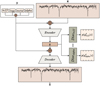 |
Fig. 1 Disentanglement architecture featuring multi-discriminators. The architecture operates as follows: spectra x and stellar parameters y are concatenated as input. The encoder then maps this concatenated input, x ⊕ y, to the latent space z, with the aim of disentangling y from z. Subsequently, the decoder’s task is to reconstruct x using z ⊕ y as input. In parallel, discriminators receive z as input and endeavour to predict the astrophysical parameters within a discretised space yd. |
2.1.2 Implementation
We employed grid search techniques to determine the model’s optimal configuration and identify suitable setups. We analysed the reconstruction errors versus the discriminators’ errors, to maintain a balance between them. We selected the size of the latent space by evaluating the relationship between size and the information loss during the reconstruction. Additionally, we used GANDALF to facilitate swift parameter adjustments for both the model and the training process. The configuration employed for the results presented in this study is outlined below.
Based on the tests, the encoder, decoder, and discriminators were constructed as fully connected neural networks. The encoder comprises two hidden layers with 512 and 256 neurons, respectively. Its output layer, representing the latent space (z), consists of 25 neurons. Conversely, the decoder mirrors the encoder’s configuration, featuring two hidden layers with 256 and 512 neurons, respectively. The input size may vary depending on the number of astrophysical parameters to be disentangled, with a base size of 25 + n_params. All discriminators share the same structure, with two hidden layers comprising 64 and 32 neurons, respectively. The output size of the discriminators is contingent upon the number of bins utilised for discretisation; in this instance, ten bins per parameter were employed.
In the multi-discriminator approach, each discriminator i is assigned a λi value, which enables control over the significance attributed to eliminating each stellar parameter:
 (4)
(4)
An auto-encoder small-loss term is obtained not only when the autoencoder can reconstruct the original spectrum accurately (small lossrec) but also when the discriminator presents large errors (large  ). The balance between both loss terms is controlled by λi for each stellar parameter, which enables either the disentangling (λi > 0) or reinforcement (λi < 0) of each specific stellar parameter. We use the term entangling for the λi < 0 case, as opposed to disentangling (see Sect. 2.3 for details).
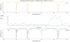 |
Fig. 2 GANDALF application to generate modified versions of an initial spectrum by adjusting the stellar parameters within the latent space. The top panel displays the original spectrum along with its four stellar parameters. The middle panel shows the latent space representation. The bottom panel shows two spectra: a new spectrum generated by setting the stellar parameters to Teff = 7500 K and [α/Fe] = 0.0 (spectrum 2) and the original spectrum reconstructed by the auto-encoder (spectrum 3), which is nearly identical to the initial input (spectrum 1). The figure is adapted from the GANDALF application. |
2.2 GANDALF framework
Our disentangling framework, GANDALF, comprises several Python classes designed for data generation, a command-line tool that facilitates model definition, training, and testing, and a web application that provides visual insights into the algorithm’s functioning. GANDALF is accessible to the community as an open-source tool hosted on GitHub1. Figure 2 illustrates our framework, which aims to empower the community to use and tailor our disentangling approach to their respective domains.
2.3 GANDALF for entangling
The GANDALF framework was built to facilitate and automate the disentangling architecture described above. Thanks to its flexibility, this architecture can be modified and adapted to different scenarios, for instance to different spectra sizes or resolutions. Beyond adjusting the architecture or altering the configuration of the networks within its structure, several training parameters can also be modified. Among them, λi, the parameter that controls the trade-off between the loss term in the reconstruction of the spectrum and the loss term of a specific discriminator, has very interesting applications. When λi is negative, the effect of the discriminator’s error on the auto-encoder’s loss function is inverted compared to when λi is positive. This means that for λi < 0, the errors of the discriminators as well as those of the spectrum reconstruction must be minimised to guarantee that the auto-encoder loss function is small. As a consequence, the training process tends to reinforce the presence of the stellar parameter i related to λi in the latent space. This ’entangling‘ technique (as opposed to disentangling) can be done with GANDALF using a simple flag. It can also be combined with the multi-discriminator approach since GANDALF allows a λi factor adjustment for each of the conditional parameters. In this way, following Eq. (4), positive values favour the elimination of a stellar parameter (disentangling) while negative values preserve their presence (entangling).
2.4 Using t-SNE to assess the level of disentanglement
The t-SNE algorithm is a statistical technique primarily employed to visualise high-dimensional data by projecting them in a lower-dimensional representation (in our case, two dimensions) in a way that preserves local relationships in the data. Specifically, t-SNE arranges similar data points close to one another on a two-dimensional map, thus placing similar spectra in proximity on the map. Since the morphology of a spectrum is influenced by stellar atmospheric parameters, highlighting the distribution of a specific stellar parameter on the t-SNE map provides a visual indication of the correlation between the shape of the spectrum and that parameter. This allows us to leverage the visual effectiveness of t-SNE to offer validation for our disentangling method. If the disentangling method effectively separates stellar parameters from other spectral information, the distribution seen after applying t-SNE to latent space representations should show no correlation, or at least a reduced correlation, with those parameters compared to the original data representation. This means that when we colour-code the objects according to the disentangled parameter in a t-SNE representation, we obtain a random distribution of colours, indicating that such a parameter is not present in the current latent representation of our objects. On the contrary, those stellar parameters that were not disentangled (or that even were entangled) condition the shape of the latent representation and if we tag their values in the t-SNE diagram, we see an ordered distribution. In Sect. 3.3, we explain how we used the t-SNE algorithm to validate the level of disentanglement obtained through generative networks using GANDALF.
3 Application of GANs to Gaia/RVS parameterisation
In June 2022, DR3 was unveiled, comprising approximately one million medium-resolution spectra from the Gaia satellite’s RVS (Recio-Blanco et al. 2023). This dataset also includes estimations of the main stellar parameters derived from these spectra. The RVS instrument generates medium-resolution spectra with R = 11 500 in the near-infrared electromagnetic spectral region. These spectra cover a wavelength range spanning from 8460 to 8700 Angstroms (Å), which focuses specifically around the lines of the calcium triplet. The analysis of RVS spectra in DR3 was carried out by Gaia Data Processing and Analysis Consortium (DPAC), the international consortium responsible for processing Gaia mission data, which extracts radial velocities and astrophysical parameters from the observations. This estimation of parameters, which we refer to as stellar parameterisation, involves a model-driven approach, where the observed spectra are interpreted through comparison with a grid of synthetic spectra (Recio-Blanco et al. 2023).
In this work, we propose a different approach that consists of a stellar parameterisation using neural networks trained not with models but with data (spectra) from a set of reference stars whose stellar atmospheric parameters have been reliably determined in the literature. In this data-driven context, we wanted to test the use of GAN with or without disentangling and entangling, to optimise the parameterisation process.
3.1 Reference stars for atmospheric stellar parameterisation
To train and test our networks, we used a reference catalogue of stars with atmospheric parameters in two large high-resolution spectroscopic surveys: APOGEE DR17 (Majewski et al. 2017; Wilson et al. 2019; Abdurro’uf et al. 2022) and GALAH DR3 (Buder et al. (2021)). Only stars in the RVS magnitude interval 8 ≤ G ≤ 14 were considered. We removed some problematic stars in both samples: those with STAR_BAD or FE_H_FLAG flagged from the APOGEE sample and those with flag_sp or flag_fe_h with values set to zero from the GALAH sample. The sample consists of 64 305 stars, most from APOGEE DR17 (54 422), complemented with 9883 from GALAH DR3. According to the parameterisation pipelines, the errors in the parameters are the following: Teff ≤ 200K; logɡ≤ 0.5 dex; and [M/H] ≤ 0.3 dex and [α/Fe] ≤ 0.2 dex. We note that APOGEE stops at −2.5 dex, which is up to where the APOGEE Stellar Parameters and Abundances Pipeline (ASPCAP) pipeline (García Pérez et al. 2016; Holtzman et al. 2018) assigns metallicities. Figure 3 shows the distribution of the four main atmospheric parameters for the reference sample of stars. Our dataset is centred on FGK giant and dwarf stars with a chemistry similar to that of the Sun. It also includes a small sample of low metallicity stars and some stars with [α/Fe] enhancement, with values around 0.3 dex. In Figs. 4 and 5, we present the Kiel diagram as well as the [M/H] versus [α/Fe] diagram for the complete dataset of reference stars.
3.2 GANDALF and DR3
When applying the GANDALF framework to create a new representation of RVS spectra, we had two main objectives. First, we aimed to improve the accuracy of the parameterisation obtained by ANN-trained regressors by using the generated latent space as input. Second, with this approach we sought to enhance inference times for parameterisation, benefiting from the more compact size of the new representation of the spectra.
To extract information from a set of observational spectra for stars with unknown atmospheric parameters, it is essential to adapt the architecture described before and shown in Fig. 1, which was initially designed for synthetic spectra. In the case of synthetic spectra, stellar parameters were introduced at the input along with the spectra. Figure 6 exemplifies the change in architecture. In this case, the stellar parameters are only concatenated with the latent space as an input for the decoder during the training phase. This architecture loses effectiveness compared to the original one but it was also much less restrictive.
As mentioned earlier, during the training phase with observed stellar spectra, the architecture in Fig. 6 was applied to a dataset with known astrophysical parameters. A model was then developed to either eliminate or preserve the conditional parameters. In the inference phase, the trained model predicted parameters for new, unseen spectra where the stellar parameters are unknown. The schematic for this phase is shown in Fig. 7. Once the encoder was trained to generate a latent space, it could process new spectra to produce their representations in that space.
3.3 Results
The training of the GANs was carried out with 51 444 spectra corresponding to 80% of the set of 64 305 reference stars, reserving the remaining 20% (12 861 spectra) for the inference phase. By using GANDALF, we computed three different latent representations of the spectra, the first one simply using the tool to construct the latent space without any parameter entanglement or disentanglement, and another two by combining the options for disentangling and entangling on parameter pairs. The pairs were selected by affinity, always grouping the physical parameters Teff and logɡ together, and the same for the chemical parameters [M/H] and [α/Fe].
Schematically, to test the effectiveness of the approach with disentangling and entangling, four data representations were considered:
- (i)
RVS spectra: The nominal RVS spectra without any dimensionality reduction.
- (ii)
Pure latent space: We disabled the influence of the four discriminators in the error calculation (λi = 0), equivalent to training a regular auto-encoder.
- (iii)
First disentangling and entangling exercise: We disentangled Teff and logɡ information from the latent space and we entangled [M/H] and [α/Fe].
- (iv)
Second disentangling and entangling exercise: We entangled Teff and logɡ information from the latent space and we disentangled the distribution of [M/H] and [α/Fe].
The t-SNE algorithm can be applied to the spectra and the corresponding latent spaces to assess the level of disentangling and entangling. For clarity, we illustrate both disentangling and entangling exercises. The t-SNE representation from the first disentangling experiment, which attempted to eliminate Teff and logɡ, is shown in panel a of Fig. 8, while the second experiment is depicted in panel b.
Figure 8 also presents the t-SNE diagram for the original spectra in the left column of the sub-figures, while the latent representations are depicted in the right columns. It is important to note that the axes of a t-SNE diagram have no physical meaning, simply reflecting the reduced representation produced by the algorithm for each object. The objects in the t-SNE diagrams are colour-coded according to their parameter values, as each figure indicates.
For example, in panel a, the top two figures show that the latent space has lost information about Teff and logɡ, whereas the bottom figures indicate that the information about [M/H] and [α/Fe] has been enhanced. Thus, t-SNE serves as a useful tool to verify the effectiveness of GANDALF in generating latent space representations with an appreciable level of disentangling or reinforcement.
Once the latent representations of the data had been obtained using GANDALF, stellar parameters for the 12 861 spectra were extracted using simple ANNs as regressors. After training, the ANNs delivered continuous estimates of the stellar parameters. The architecture is the following: the input is composed of 800 neurons (in the case of the original spectra) or 25 neurons (for the latent representations), two hidden layers of 200 and 100 neurons. The output is composed of four neurons to map the four stellar parameters. All experiments in this work were conducted using Scikit’s (Pedregosa et al. 2011) fully connected networks with backpropagation, and we maintained the same structure across all cases.
We conducted tests to train networks to predict individual parameters as well as all four parameters simultaneously. Since the results were very similar, only those for the network predicting all four stellar parameters are presented.
The results are summarised in Table 1, which shows the mean, absolute mean, and standard deviation values of the differences to the literature values for the four stellar parameters. While the statistics are generally good for both the pure latent space representation and the original spectra illustrating the effectiveness of ANNs as regressors, it is clear that using latent space representations with disentangling non-target parameters and enhancing target parameters significantly improves the outcomes. The accuracy obtained is sufficient to distinguish between dwarf and giant stars, between objects belonging either to the halo or to the thin and thick components of the galactic disc and, consequently, it is sufficiently accurate to carry out studies of stellar populations. Figures 9 and 10 show the Kiel diagram and the distribution of [M/H] versus [α/Fe] diagram obtained through entangling of the relevant parameters (Teff and logɡ in the case of the Kiel diagram and the distribution of [M/H] and [α/Fe] for the other diagram) and disentangling of the other pair of parameters. Regarding computational times, a threefold reduction is achieved when training the regressors with the optimised latent space instead of the original spectra over 1000 iterations on a six-core desktop computer, an Intel Core i7 8700 at 3.20 GHz, and 96 GB of RAM.
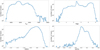 |
Fig. 3 Distribution of the four main stellar atmospheric parameters in our sample of stars. Values are from APOGEE DR17 and GALAH DR3. |
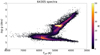 |
Fig. 4 Kiel diagram showing the gravity (logɡ) against the effective temperature (Teff ) for the selected sample of reference stars, with parameter values obtained from APOGEE DR17 and GALAH DR3. Readers can refer to the main text for details. |
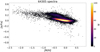 |
Fig. 5 Distribution of [M/H] versus [α/Fe] for the sample of reference stars, with parameter values obtained from APOGEE DR17 and GALAH DR3. Readers can refer to the main text for details. |
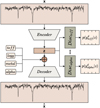 |
Fig. 6 Schematic of the adversarial network for a case where the value of the astrophysical parameters cannot be provided as input. |
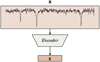 |
Fig. 7 Schematic of the inference phase. Once the adversarial network is trained, the encoder is used to produce the latent space (z) of sample spectra with unknown stellar parameters. |
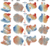 |
Fig. 8 t-SNE diagram obtained for the two disentangling exercises. The column panels (a) refer to the first disentangling exercise, in which we tried to eliminate the contribution of the physical parameters (Teff and logɡ) in the latent space and reinforce the influence of the chemicals ones ([M/H] and [α/Fe]). The inverse case is shown in column (b). Each panel illustrates the t-SNE result on the original spectrum (sub-figures on the left) and the latent space (on the right) corresponding to each disentangling exercise. The figures are colour-coded according to the values of the parameters, as indicated in each figure. |
Summary statistics obtained for parameterisation using different representations of the input space.
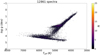 |
Fig. 9 Kiel diagram for test stars obtained after parameterisation with latent spaces using entangling for Teff and logɡ, and disentangling for the distribution of [M/H] and [α/Fe]. |
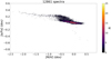 |
Fig. 10 Distribution of [M/H] versus [α/Fe] diagram for test stars obtained after parameterisation by entangling of [M/H] and [α/Fe], and disentangling Teff and logɡ. |
4 Conclusions
Discovering data representations that facilitate the extraction of useful information and enhance algorithm performance in classification and parameterisation problems is essential in the context of extensive spectroscopic astronomical surveys. This work introduces an encoder-decoder architecture that features a modification of the traditional auto-encoder with adversarial training. The objective is to disentangle the desired parameters from the rest of the information contained in astronomical spectra within the latent space produced by the encoder. Specifically, we developed an algorithm for the physicochemical disentanglement of information present in the RVS Gaia spectroscopic survey. By projecting the signal (stellar spectra) into a latent space where contributions from physical properties (Teff and logɡ) were minimised, we could maximise the information related to chemical properties, thereby improving their extraction. The disentangling of atmospheric chemical parameters [M/H] and [α/Fe] also enhances the precision in the derivation of physical parameters. We visualised the level of disentanglement in the latent space using the t-SNE algorithm. Beyond its initial application, we believe that our methodology can significantly impact big data astronomy, especially given the rise of modern all-sky spectroscopic surveys, since our algorithm offers substantial data dimensionality reduction while preserving and even highlighting key information. Additionally, our method can be used to efficiently interpolate and extrapolate samples beyond the input data range, which is useful for validation or for creating new synthetic spectral grids. To implement this, we developed an ad hoc framework called GANDALF. This framework includes several Python classes for data generation, command line tools for model definition, training, and testing, and a web application to visually demonstrate the algorithm. GANDALF is available to the community as an open-source tool on GitHub.
Acknowledgements
Horizon Europe funded this research [HORIZON-CL4-2023-SPACE-01-71] SPACIOUS project, Grant Agreement no. 101135205, the Spanish Ministry of Science MCIN/AEI/10.13039/501100011033, and the European Union FEDER through the coordinated grant PID2021-122842OB-C22. We also acknowledge support from the Xunta de Galicia and the European Union (FEDER Galicia 2021–2027 Program) Ref. ED431B 2024/21, CITIC ED431G 2023/01, and the European Social Fund – ESF scholarship ED481A2019/155.
References
- Abazajian, K. N., Adelman-McCarthy, J. K., Agüeros, M. A., et al. 2009, ApJS, 182, 543 [Google Scholar]
- Abdurro’uf, Accetta, K., Aerts, C., et al. 2022, ApJS, 259, 35 [NASA ADS] [CrossRef] [Google Scholar]
- Bailer-Jones, C. A. L., Irwin, M., & von Hippel, T. 1998, MNRAS, 298, 361 [NASA ADS] [CrossRef] [Google Scholar]
- Barbara, N. H., Bedding, T. R., Fulcher, B. D., Murphy, S. J., & Van Reeth, T. 2022, MNRAS, 514, 2793 [NASA ADS] [CrossRef] [Google Scholar]
- Baron, D., & Poznanski, D. 2017, MNRAS, 465, 4530 [NASA ADS] [CrossRef] [Google Scholar]
- Bengio, Y., Courville, A., & Vincent, P. 2013, IEEE Trans. Pattern Anal. Mach. Intell., 35, 1798 [CrossRef] [Google Scholar]
- Bishop, C. M. 2006, Pattern Recognition and Machine Learning (Springer) [Google Scholar]
- Buder, S., Sharma, S., Kos, J., et al. 2021, MNRAS, 506, 150 [NASA ADS] [CrossRef] [Google Scholar]
- Chen, X., Duan, Y., Houthooft, R., et al. 2016, arXiv e-prints [arXiv:1606.03657] [Google Scholar]
- Cheung, B., Livezey, J. A., Bansal, A. K., & Olshausen, B. A. 2015, arXiv eprints [arXiv:1412.6583] [Google Scholar]
- Cover, T. M., & Joy, T. J. A. 2006, Elements of Information Theory, 2nd edn. (Hoboken, New Jersey: John Wiley & Sons, Inc.) [Google Scholar]
- Dafonte, C., Garabato, D., Alvarez, M. A., & Manteiga, M. 2018, Sensors, 18, 1418 [Google Scholar]
- Delchambre, L., Bailer-Jones, C. A. L., Bellas-Velidis, I., et al. 2023, A&A, 674, A31 [NASA ADS] [CrossRef] [EDP Sciences] [Google Scholar]
- de Mijolla, D., & Ness, M. K. 2022, ApJ, 926, 193 [NASA ADS] [CrossRef] [Google Scholar]
- de Mijolla, D., Ness, M. K., Viti, S., & Wheeler, A. J. 2021, ApJ, 913, 12 [NASA ADS] [CrossRef] [Google Scholar]
- Gaia Collaboration (Prusti, T., et al.) 2016, A&A, 595, A1 [NASA ADS] [CrossRef] [EDP Sciences] [Google Scholar]
- García Pérez, A. E., Allende Prieto, C., Holtzman, J. A., et al. 2016, AJ, 151, 144 [Google Scholar]
- Garvin, E. O., Bonse, M. J., Hayoz, J., et al. 2024, A&A, 689, A143 [NASA ADS] [CrossRef] [EDP Sciences] [Google Scholar]
- Goodfellow, I. J., Pouget-Abadie, J., Mirza, M., et al. 2014, arXiv e-prints [arXiv:1406.2661] [Google Scholar]
- Holtzman, J. A., Hasselquist, S., Shetrone, M., et al. 2018, AJ, 156, 125 [Google Scholar]
- Hughes, A. C. N., Bailer-Jones, C. A. L., & Jamal, S. 2022, A&A, 668, A99 [NASA ADS] [CrossRef] [EDP Sciences] [Google Scholar]
- Lake, B. M., Ullman, T. D., Tenenbaum, J. B., & Gershman, S. J. 2017, Behav. Brain Sci., 40, e253 [CrossRef] [Google Scholar]
- Lample, G., Zeghidour, N., Usunier, N., et al. 2018, arXiv e-prints [arXiv:1706.00409] [Google Scholar]
- Majewski, S. R., Schiavon, R. P., Frinchaboy, P. M., et al. 2017, AJ, 154, 94 [NASA ADS] [CrossRef] [Google Scholar]
- Mathieu, M., Zhao, J., Sprechmann, P., Ramesh, A., & LeCun, Y. 2016, arXiv e-prints [arXiv:1611.03383] [Google Scholar]
- Pedregosa, F., Varoquaux, G., Gramfort, A., et al. 2011, J. Mach. Learn. Res., 12, 2825 [Google Scholar]
- Price-Jones, N., & Bovy, J. 2019, MNRAS, 487, 871 [NASA ADS] [CrossRef] [Google Scholar]
- Recio-Blanco, A., de Laverny, P., Palicio, P. A., et al. 2023, A&A, 674, A29 [NASA ADS] [CrossRef] [EDP Sciences] [Google Scholar]
- Re Fiorentin, P., Bailer-Jones, C. A. L., Lee, Y. S., et al. 2007, A&A, 467, 1373 [NASA ADS] [CrossRef] [EDP Sciences] [Google Scholar]
- Rifai, S., Bengio, Y., Courville, A., Vincent, P., & Mirza, M. 2012, in Computer Vision–ECCV 2012: 12th European Conference on Computer Vision, Florence, Italy, October 7–13, 2012, Proceedings, Part VI 12 (Springer), 808 [CrossRef] [Google Scholar]
- Santoveña, R., Dafonte, C., & Manteiga, M. 2024, arXiv e-prints [arXiv:2411.05960] [Google Scholar]
- Shallue, C. J., & Vanderburg, A. 2018, AJ, 155, 94 [NASA ADS] [CrossRef] [Google Scholar]
- Szabó, A., Hu, Q., Portenier, T., Zwicker, M., & Favaro, P. 2017, arXiv e-prints [arXiv:1711.02245] [Google Scholar]
- Tardugno Poleo, V., Eisner, N., & Hogg, D. W. 2024, AJ, 168, 100 [CrossRef] [Google Scholar]
- van der Maaten, L., & Hinton, G. 2008, J. Mach. Learn. Res., 9, 2579 [Google Scholar]
- Wang, X., Chen, H., Tang, S., Wu, Z., & Zhu, W. 2024, IEEE Trans. Pattern Anal. Mach. Intell., 1 [Google Scholar]
- Wilson, J. C., Hearty, F. R., Skrutskie, M. F., et al. 2019, PASP, 131, 055001 [NASA ADS] [CrossRef] [Google Scholar]
All Tables
Summary statistics obtained for parameterisation using different representations of the input space.
All Figures
|
Fig. 1 Disentanglement architecture featuring multi-discriminators. The architecture operates as follows: spectra x and stellar parameters y are concatenated as input. The encoder then maps this concatenated input, x ⊕ y, to the latent space z, with the aim of disentangling y from z. Subsequently, the decoder’s task is to reconstruct x using z ⊕ y as input. In parallel, discriminators receive z as input and endeavour to predict the astrophysical parameters within a discretised space yd. |
| In the text | |
|
Fig. 2 GANDALF application to generate modified versions of an initial spectrum by adjusting the stellar parameters within the latent space. The top panel displays the original spectrum along with its four stellar parameters. The middle panel shows the latent space representation. The bottom panel shows two spectra: a new spectrum generated by setting the stellar parameters to Teff = 7500 K and [α/Fe] = 0.0 (spectrum 2) and the original spectrum reconstructed by the auto-encoder (spectrum 3), which is nearly identical to the initial input (spectrum 1). The figure is adapted from the GANDALF application. |
| In the text | |
|
Fig. 3 Distribution of the four main stellar atmospheric parameters in our sample of stars. Values are from APOGEE DR17 and GALAH DR3. |
| In the text | |
|
Fig. 4 Kiel diagram showing the gravity (logɡ) against the effective temperature (Teff ) for the selected sample of reference stars, with parameter values obtained from APOGEE DR17 and GALAH DR3. Readers can refer to the main text for details. |
| In the text | |
|
Fig. 5 Distribution of [M/H] versus [α/Fe] for the sample of reference stars, with parameter values obtained from APOGEE DR17 and GALAH DR3. Readers can refer to the main text for details. |
| In the text | |
|
Fig. 6 Schematic of the adversarial network for a case where the value of the astrophysical parameters cannot be provided as input. |
| In the text | |
|
Fig. 7 Schematic of the inference phase. Once the adversarial network is trained, the encoder is used to produce the latent space (z) of sample spectra with unknown stellar parameters. |
| In the text | |
|
Fig. 8 t-SNE diagram obtained for the two disentangling exercises. The column panels (a) refer to the first disentangling exercise, in which we tried to eliminate the contribution of the physical parameters (Teff and logɡ) in the latent space and reinforce the influence of the chemicals ones ([M/H] and [α/Fe]). The inverse case is shown in column (b). Each panel illustrates the t-SNE result on the original spectrum (sub-figures on the left) and the latent space (on the right) corresponding to each disentangling exercise. The figures are colour-coded according to the values of the parameters, as indicated in each figure. |
| In the text | |
|
Fig. 9 Kiel diagram for test stars obtained after parameterisation with latent spaces using entangling for Teff and logɡ, and disentangling for the distribution of [M/H] and [α/Fe]. |
| In the text | |
|
Fig. 10 Distribution of [M/H] versus [α/Fe] diagram for test stars obtained after parameterisation by entangling of [M/H] and [α/Fe], and disentangling Teff and logɡ. |
| In the text | |
Current usage metrics show cumulative count of Article Views (full-text article views including HTML views, PDF and ePub downloads, according to the available data) and Abstracts Views on Vision4Press platform.
Data correspond to usage on the plateform after 2015. The current usage metrics is available 48-96 hours after online publication and is updated daily on week days.
Initial download of the metrics may take a while.