| Issue |
A&A
Volume 694, February 2025
|
|
|---|---|---|
| Article Number | A188 | |
| Number of page(s) | 19 | |
| Section | The Sun and the Heliosphere | |
| DOI | https://doi.org/10.1051/0004-6361/202449289 | |
| Published online | 11 February 2025 | |
Magnetic connectivity of coronal loops and flare-accelerated electrons in a B-class flare
Based on X-ray, EUV (DEM analysis), and type-III radio burst observations
1
Leibniz Institute for Astrophysics Potsdam (AIP), An der Sternwarte 16, 14482 Potsdam, Germany
2
Zentrum für Astronomie und Astrophysik, Technische Universität Berlin, Hardenbergstraße 36, 10623 Berlin, Germany
3
Space Radio-Diagnostics Research Centre, University of Warmia and Mazury, R. Prawocheńskiego 9, 10-719 Olsztyn, Poland
4
Center for mathematical Plasma Astrophysics, Department of Mathematics, Katholieke Universiteit Leuven, Celestijnenlaan 200B, 3001 Leuven, Belgium
5
Solar-Terrestrial Centre of Excellence, Royal Observatory of Belgium, Avenue Circulaire 3, 1180 Uccle, Belgium
6
RAL Space, United Kingdom Research and Innovation – Science & Technology Facilities Council – Rutherford Appleton Laboratory, Harwell Campus, Oxfordshire OX11 0QX, UK
7
Polish Academy of Sciences, Palace of Culture and Science, Pl. Defilad 1, 00-901 Warsaw, Poland
8
ASTRON, Netherlands Institute for Radio Astronomy, Oude Hoogeveensedijk 4, 7991 PD Dwingeloo, The Netherlands
⋆ Corresponding authors; This email address is being protected from spambots. You need JavaScript enabled to view it.
, This email address is being protected from spambots. You need JavaScript enabled to view it.
Received:
19
January
2024
Accepted:
7
December
2024
Abstract
Context. In solar flares, non-potential magnetic field energy is transferred to particle acceleration, heating, and radiation. Multi-wavelength observations of the solar corona in extreme ultraviolet (EUV) and X-ray show the consequences of magnetic reconfiguration in lower heights, while radio observations contain information about the access of flare-accelerated electrons to greater heights in the solar atmosphere. Signs of downward and upward particle propagation do not always appear symmetrically, they depend on the acceleration process, the sensitivity of the instruments, and the magnetic connectivity. The magnetic connectivity in various flare phases is therefore a key element to study in order to gain a better understanding of combined flare observations.
Aims. We aim to draw conclusions about the magnetic connectivity of specific coronal loops in the active region, the acceleration region, and the higher corona with respect to different phases of the flare process.
Methods. We investigate the evolution of particle acceleration, loops heated by the energy release, and the trajectories of flare-accelerated electrons observed up to one solar radius (1 RS) above the active region in a B-class flare on 6 June 2020. We studied the downward particle acceleration and thermal evolution with observations by the Spectrometer/Telescope for Imaging X-rays and with a reconstruction code based on EUV observations. Traces of flare-accelerated electrons, namely, type-III radio bursts, were investigated with a spectroscopic solar dynamic radio imager (LOw Frequency ARray). The radio source positions in heights of 0.4 RS–1.0 RS were compared with the thermal evolution of coronal loops and with a solar magnetic field model.
Results. In this flare event, similar magnetic reconnection processes and accompanied heating processes are triggered several times. For loops and periods with access to the higher corona, type-III bursts from similar reconnection process are emitted along similar propagation trajectories. There are no radio bursts associated with the heating process of the main flaring loop.
Conclusions. In this event, the large-scale magnetic field is rather stable and seems not to be affected by the flare. The access to loops reaching heights of half a solar radius or more is suppressed during the main flare phase for flare-accelerated electrons. This may lead to more effective heating and absent type-III radio bursts between 20 MHz and 85 MHz.
Key words: Sun: activity / Sun: corona / Sun: flares / Sun: magnetic fields / Sun: radio radiation
© The Authors 2025
 Open Access article, published by EDP Sciences, under the terms of the Creative Commons Attribution License (https://creativecommons.org/licenses/by/4.0), which permits unrestricted use, distribution, and reproduction in any medium, provided the original work is properly cited.
This article is published in open access under the Subscribe to Open model. This email address is being protected from spambots. You need JavaScript enabled to view it. to support open access publication.
1. Introduction
The solar magnetic field stores energy in twisted and sheared coronal loops, which is suddenly released during impulsive events called solar flares. The initial particle acceleration at shock fronts and in the magnetic reconnection region is linked to heating of coronal plasma to several megakelvins (MK) and radiation across the electromagnetic spectrum (standard flare model; Carmichael 1964; Sturrock & Coppi 1966; Hirayama 1974; Kopp & Pneuman 1976).
Flare-accelerated electrons propagate along the magnetic field lines toward the Sun and collide with denser material, which leads to chromospheric evaporation at the foot points. Hard X-ray radiation is emitted, and the participating loops are filled with hot plasma visible in soft X-ray and extreme ultraviolet (EUV) wavelengths. The system of loops participating in the flare process is referred to as an active region (AR).
Flare-accelerated electrons also propagate away from the Sun through the gravitationally stratified solar atmosphere (Ginzburg & Zhelezniakov 1958) and lead to unstable velocity distributions along their trajectory. Consequently, Langmuir waves are generated close to the local plasma frequency and are then transformed into radio waves (Zheleznyakov & Zaitsev 1970; Lin 1974; Melrose 1985). The characteristic signals in dynamic radio spectra are the solar type-III radio bursts reported by Wild (1950). Type-III radio bursts are characterized by high frequency drift rates, a result of a high velocity of the electron beams, and the emission of radio waves close to the local plasma frequency or its harmonics (e.g., Melrose 1985; Reid 2020). When electrons follow closed magnetic fields, they can produce U- or J-bursts (Maxwell & Swarup 1958).
By assuming this rather symmetric flare process in which some of the electrons are accelerated outward and the others downward, the LOw Frequency ARray (LOFAR; van Haarlem et al. 2013) and the Spectrometer/Telescope for Imaging X-rays (STIX; Krucker et al. 2020) therefore observe each other’s counterpart of flare-accelerated electrons. One-to-one relations in single events (Kane et al. 1982) are supported by various studies, which have found correlations between hard X-ray radiation and type-III bursts (Kane 1972; Kundu et al. 1980; Reid et al. 2011; James & Vilmer 2023). Maxima of hard X-rays and type-III solar radio bursts in the 10 MHz–580 MHz range (when detectable) agree in their timing within ±9 s (Kane 1972). However, the differences in emission mechanisms between radio and X-ray may reduce the correlation of the two kinds of observations.
Type-III radio bursts can generally be considered as very sensitive indicators for changes in the AR. The number of electrons producing type-III bursts is only around 0.1% of the number of electrons necessary to produce X-rays (Lin et al. 1973; Krucker et al. 2007; James & Vilmer 2023), a possible explanation for the appearance of many type-III radio bursts without an X-ray counterpart. There are ARs without significant flares, which were found to be the source of electron beams causing a type-III radio noise storm (Harra et al. 2021). Large flare events are therefore not a requirement for the appearance of radio bursts.
The opposite case, namely X-ray radiation in flares without type-III bursts, can typically not be explained by sensitivity effects. Instead, it indicates the absence of flare-accelerated electrons in greater solar heights. Since charged particles follow the magnetic field lines, the coronal field determines the paths of the electrons.
How exactly electrons end up on specific closed or open magnetic field lines during flares is still an open question. The electron trajectories depend on the magnetic connectivity of the acceleration region, the AR, and the higher corona, that is, the incorporation of small-scale processes leading to particle acceleration in the large-scale magnetic structures (Raulin et al. 2000). Magnetic typologies involved in flare evolution can be complex at all spatial scales. In this context, stepwise temporal evolutions of the flare-accelerated electrons have been found to be related to similar stepwise variations of the magnetic structures illuminated by hot plasma, while the acceleration region associated with a hard X-ray source stays in the same position (Raulin et al. 2000). Both aspects, namely the relations of heating and particle acceleration and the position of the acceleration region in different types of AR, are still fields of ongoing research.
In this paper, a flare event with a rather simple AR and stable large-scale magnetic field is analyzed. While this general setup remains constant, the correlation of X-ray and radio observations is analyzed. The simplicity of the event with several triggered acceleration processes during the flare phases enabled us to identify both the heated coronal loops and flare-accelerated electrons as likely being related to a similar reconnection process. We compare the small-scale structural and thermal changes of these coronal loops with source positions of 18 type-III radio bursts in heights between 0.4 RS and 1.0 RS (solar radius) above the AR.
Type-III emitting electrons have been found to have a direct connectivity to the reconnection region (Chen et al. 2013). We investigate whether these electrons access similar field lines or change their trajectories during the different flare phases. With our analysis, we aim to draw conclusions about the evolution of the magnetic connectivity of these regions, which implies a high importance for a better understanding of flare processes in 3D (Caspi et al. 2023) and space weather in general.
2. Methods
In this paper, data from various space- and ground-based instruments are used to perform a multi-wavelength analysis of a flare event. Additionally, we used a model of the coronal magnetic field as context information. We compared the thermal evolution with the particle acceleration and propagation. Our analysis techniques differ from previous studies (mainly Benz et al. 1983; Raulin et al. 2000; Trottet 2003; Trottet et al. 2006) in a way, as we make use of spatially resolved differential emission measure reconstruction techniques (based on highly resolved EUV data). With these analysis tools, the sensitivity is also given for smaller energy releases, which are too small to become visible in the X-ray observations. By deriving spatially resolved emission measure (EM) and EM-weighted temperature maps, electron propagation and thermal evolution of the AR can be investigated side by side. The previous studies mentioned focus mainly on higher frequencies (above 150 MHz) and use the Nançay Radioheliograph. However, in this work, we utilize a dynamic imaging radio spectrometer (LOFAR) for radio bursts below 80 MHz, which corresponds to heights above 0.43 RS (based on the used density model by Mann et al. 1999, Sect. 4.2).
2.1. X-ray instruments GOES and STIX
We use the X-ray detector on the Geostationary Operational Environmental Satellite (GOES) for spatially unresolved data. Additionally, STIX is used, which belongs to the remote sensing instruments of the Solar Orbiter mission (Müller et al. 2020). STIX was designed for hard X-rays imaging spectroscopy (Krucker et al. 2020).
2.2. Differential emission measure reconstruction from extreme ultraviolet data
For EUV observations we use AIA (Lemen et al. 2012) on board NASA’s Solar Dynamics Observatory (SDO). The instrument is a full-disk EUV imager with 1.5″ spatial resolution and 12 s temporal resolution and takes images in seven EUV band passes.
The coronal plasma reacts to the dynamic processes in the flare and evolves in time. We extract the full temperature information contained in the intensity data of the multi-thermal AIA channels by applying a differential emission measure (DEM) reconstruction code (Cheung et al. 2015; Su et al. 2018).
The DEM reconstruction is a method for disentangling density and temperature-induced brightening in EUV images by using the six EUV channels with different temperature response function. A 3 × 3 binning of the AIA data was used as the input data. The DEM describes the amount of thermal plasma along the line of sight as a function of temperature T (e.g., Su et al. 2018).
DEM and emission measure EMT within a certain temperature bin ΔT are related by
 (1)
(1)
where ne is the electron number density and z is the distance along the line of sight. The temperature range of the DEM analysis spans from 105.2 K to 107.5 K, an interval which is adequately covered by the six iron line channels of AIA. EM is reconstructed for temperature bins with a size of log10T equal to 0.05.
EM-weighted temperatures, TEM, can be then derived from the DEM distribution by
 (2)
(2)
where EM is the summed EM from all temperature bins.
The lower temperature limit was set to 1.6 MK to highlight the evolution of the actual flare plasma, rather than the background. Pixels outside the temperature range are excluded from the analysis and are displayed in black (Fig. 5). ‘Hot pixels’ occur in areas with very low EM. Because the method used is pixel independent, the other parts of the image are not affected and can still be used for the analysis. Nevertheless, the input data in all six AIA channels should be free of any saturation for avoiding loss of information about the full thermal evolution. Especially in larger events, saturation is an issue around the flare peak. We avoid this limitation by choosing a B-class flare for the analysis. The pixel-based DEM routine preserves the spatial information of the AIA input data and provides detailed EM and temperature maps.
2.3. LOFAR
Propagation paths of flare-accelerated electrons can be indirectly observed by the analysis of solar radio radiation (Aschwanden 2004, as a review). We use data from LOFAR (van Haarlem et al. 2013). The European radio interferometer consists of 52 stations, 24 core stations, 14 remote stations in the Netherlands and 14 international stations located in: France, Germany, Ireland, Latvia, Poland, Sweden, and the United Kingdom. Each station collects data with Low Band Antennas (LBA, i.e. 10 MHz–90 MHz) and High Band Antennas (HBA, i.e. 110 MHz–250 MHz).
LOFAR as a spectroscopic solar dynamic radio imager measures positions and fluxes of radio sources at each frequency over time. The temporal resolution of the dynamic spectra (up to 0.01 s) and imaging (0.25 s) is high enough to even resolve the fine structure of radio bursts (Reid & Kontar 2021; Dabrowski et al. 2025). Since radio waves with a certain frequency are only emitted from a specific height in the solar atmosphere, the set of images show the trajectory of flare-accelerated electrons. It allows us to track electron beams through the solar corona (Mann et al. 2018). The data was recorded under proposal LT16_001 “Advancing solar and heliospheric physics with LOFAR in the era of Parker Solar Probe and Solar Orbiter”, prepared by the Solar and Space Weather Key Science Project.
The radio sources are imaged by using the Solar Imaging Pipeline by Breitling et al. (2015). This software package was developed at Leibniz Institute for Astrophysics Potsdam (AIP) and is based on the LOFAR Standard Imaging Pipeline by Heald et al. (2011). Simultaneous observation of the Sun and a calibrator are conducted to calibrate the interferometric data. That allows us to study the evolution of absolute radio fluxes. After the calibration with Cygnus A the corrected data is imaged with the multi-scale CLEAN algorithm provided by CASA (McMullin et al. 2007). For a suitable visualization, we present the radio images as contours at the full width at half maximum. The selected frequencies are 80 MHz (purple), 70 MHz (blue), 60 MHz (green), 50 MHz (orange) and 40 MHz (red). The decision is based on the occurrence of type-III bursts in the dynamic radio spectra between 80 MHz and 40 MHz. Between these frequencies there is also spatially resolved data available, but not displayed here to enhance the clarity of the text by reducing the complexity of the presented data for the reader.
The propagation directions are described in the entire manuscript in the same way as the apparent movement on the solar disk with 0° as north, 180° as south, 90° as west and 270° as east.
2.4. Potential-field source-surface model
To connect the LOFAR observations with data from the low corona information about the magnetic configuration is needed. Due to limited magnetic field information in the corona, photospheric data is used to model the full solar magnetic field for the regions above it. The potential-field source-surface (PFSS) model of the solar magnetic field provides information about the global morphology of the coronal magnetic field and is based on the Helioseismic and Magnetic Imager (HMI) observations on SDO (Handy & Schrijver 2001; Schrijver et al. 2003). The PFSS model used in this paper is part of the SolarSoftWare (SSW, Freeland & Handy 1998). The graphical user interface provides different input parameters as the start height or the considered area of the HMI data. It is a simple and well tested model, which is used to visualize the magnetic field lines in the observed region as a context information about the magnetic connection between sources.
3. Observations
In this section we present the multi-wavelength observations and start with the used nomenclature and an overview of the flare event based on X-ray data. In the first half of this section, all data from the AR in the lower corona is presented. In the second half, we continue with the radio observations of flare-accelerated electrons in the higher corona.
3.1. Nomenclature
We introduce the following naming for features in EUV, DEM, X-ray and radio observations. Each feature, (i.e., EUV enhancements, temperature or EM increases, X-ray peaks or radio bursts), is named with a combination of letters and sub- and superscripts to make it easier to compare the detailed data. Subscripts are used for the pre-flare phase (0), first flare phase (1), second flare phase (2), and gradual phase (g). The EUV and DEM features are named after their location within one of the main loops: a, b, c. These are in principle loop systems consisting of several sub-loops. For example, a12 is the second feature in loop a in the first flare phase, while Tag stands for a temperature increase in loop a in the gradual phase. Primes are used (e.g., X0’) if there are numerous X-ray peaks in the same flare phase. Radio bursts are denoted with a capital “R” and are successively numbered in each flare phase. If the radio burst was observed already in a previous flare phase, we kept the previous number and distinguish them with a subscript. Superscripts are used when a similar burst appears repeatedly (e.g., R501 to R507).
3.2. X-ray fluxes
The GOES satellite registered a B1 solar flare originating from NOAA AR 12765 from 08:39 UT to 09:01 UT on 6 June 2020. The flare is characterized by two major peaks in the soft X-rays (Fig. 1, 1 Å − 8 Å), at 08:42 UT (X1) and 08:47 UT (X2). Two minor peaks are observed in the pre-flare phase at 08:32:30 UT (X0) and right before the flare onset at 08:39:30 UT in GOES (X0’). Slopes of the X-ray fluxes are the steepest before X0 and X1. The fluxes evolve gradually before X0’ and X2. The channel 1 Å − 8 Å shows mainly the thermal evolution of the flare.
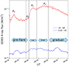 |
Fig. 1. Smoothed GOES X-ray fluxes in 1 Å − 8 Å and 0.5 Å − 4 Å. Flare phases are marked with black vertical lines between the flare onset at 08:40 UT and the second flare onset at 08:44 UT and between the second flare onset and the peak X-ray flux at 08:47 UT. The dashed line highlights the onset of the main group of type-III radio bursts (08:38:30 UT–08:40 UT) at the end of the pre-flare phase. |
The signal-to-noise ratio is very low for the higher energy channel (0.5 Å − 4 Å), the flare did not produce significant hard X-ray radiation, due to the rather small size of the flare event. The smoothed data (spline interpolation) is shown for completeness, but it is not used for the analysis due to the low fluxes.
It was not possible to reconstruct images due to the low flux, since the selected event is at the lower boundary of STIX’s sensitivity. Therefore, the source of X-rays must be determined with other data sets. STIX detected most X-rays in the energy range of 6 keV–7 keV (Fig. 7). While the energies are often classified as thermal radiation, this energy range can contain both thermal and non-thermal components in this event.
The Neupert theorem relates the hard X-ray flux and the derivative of soft X-ray flux (Neupert 1968). The energy release due to deacceleration of electrons at the foot points is proportional to the heating rate of the coronal loops bridging the foot points. We have included the derivative of the X-ray curve (6 keV–7 keV) to show where the hard X-ray radiation is expected, if the flare event itself would have been stronger. The peaks of the derivative occur at 08:38 UT, 08:40 UT and 08:44 UT.
Based on the X-ray fluxes, the flare is divided into the “pre-flare phase” (08:30 UT–08:40 UT), accompanied by the minor X-ray peaks (X0, X0’); the “first flare phase” (08:40 UT–08:44 UT); and the “second flare phase” (08:44 UT–08:50 UT). The “gradual phase” begins at 08:50 UT after reaching X2.
3.3. General magnetic field configuration
AR 12765 is located in the south at the eastern limb (x = [ − 700 : −540], y = [ − 350 : −460]) of the Sun (Fig. 2). The solar magnetic field combines several contributions in it. Below the AR there are regions of positive and negative polarity connected by coronal magnetic field lines (Fig. 2, HMI data). AIA observations show the evolution of the AR over time. Observations in a cooler channel 171 Å (5.2 to 6.2 log T) and a hotter channel 94 Å (5.6 to 5.3 log T and 6.5 to 7.1 log T) are displayed in Fig. 4. Differences in the evolution between shorter loops (a, b, c, A-B, length < 40 Mm), and longer loops show, that the AR consists of an extended static loop systems of medium size (M, length ≈2 ⋅ 102 Mm) above a smaller set of mainly three heated core loops (a, b, c) with dynamic activity.
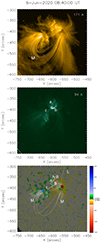 |
Fig. 2. AIA observations in two channels and HMI data show the coronal loops of the AR with different sizes and magnetic polarities. Top panel: Magnetic field lines in channel 171 Å. Middle panel: Magnetic field lines in channel 94 Å. This channel shows mainly the small-scale loops of the AR. Larger loops with lower temperatures are only faintly visible. Bottom panel: Colorized magnetogram based on HMI data showing the different polarities of the AR. The overlaid illustrations of possible loops were identified by eye from the AIA observations. |
Far-reaching field lines (L) are not filled with enough plasma to become visible in the AIA images, but are expected to originate from the regions of strong positive or negative polarity (HMI magnetogram in Fig. 2 or Fig. 3) toward another AR about one solar radius in north west direction.
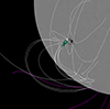 |
Fig. 3. PFSS model for a starting height of 1.01 solar radii and a projection centroid of L0 = 100° and B0 = −30°. Displayed in green are data from channel 94 Å (AIA) to complement the model. |
From a global perspective there are mainly open solar magnetic field lines at the poles and closed ones between the poles (i.e., the dipole character of the solar magnetic field). Also, the PFSS model contains these aspects of the large-scale solar magnetic field, by increasing the start height of the simulation one emphasizes the far-reaching field lines. The only open field lines relevant for the presented AR (purple, Fig. 3) can be found at the south pole. The model shows closed magnetic field lines connecting the poles and the eastern part of the ARs, where also the large-scale field lines of the AR have one part of their foot points. The field lines are orientated in south-west direction. The western part of far-reaching field lines connect either to the north pole or to the other AR, which can be seen in Fig. 11. There are no open field lines in this region.
EUV observations by AIA (Fig. 2, 171 Å) confirm the east-west orientation of the extended coronal loops (M) connecting regions of different polarity. These observations highlight the mid-scale magnetic field of the AR. Smaller scales are not easily resolved by PFSS model, but can be directly observed with the EUV observations. The loops a, b and c are situated in the core of the total magnetic field consisting of encapsulated loop systems. LOFAR LBA observations cover a part of the large-scale loops L, with loop heights above 0.4 RS.
3.4. Evolution of the active region
The evolution of the AR as seen from EUV observations (cf. attached movie and Fig. 4) is described for each flare phase. We concentrate on the small-scale loop system in lower heights (Fig. 4), because loops a, b and c exhibit most of the activity in this event. For those loops both spatially resolved DEM maps (EM and EM-weighted temperatures) and average values of selected sub-regions are discussed here.
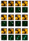 |
Fig. 4. AIA observations in 171 Å and 94 Å of the small-scale AR with the main loops a, b, c, and A-B. White circles indicate the foot points of the overlaying M and L loops (Fig. 2). Enhancements of intensities are marked with red dots and white boxes. These highlight foot points and loop-tops of the suddenly changing loops. Red arrows show the orientation of the loops based on the polarity of their foot points (HMI data, Fig. 2). The associated movie is available online. |
Since the event did not produce strong enough X-rays to use STIX imaging capabilities, the DEM reconstruction is particularly useful in this case. By focusing on the higher temperature range, the spatial information can also be obtained by the DEM analysis. During the reconfiguration of the AR and resulting X-ray peaks (X0–X2), we search for any indication of primary energy release in the loops (e.g., foot point) heating, and their thermal response in the time thereafter as seen from the DEM map analysis (Fig. 5). Based on the standard flare model, these processes are triggered by magnetic reconnection.
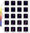 |
Fig. 5. Evolution of the core loops of the AR as seen in the EM-weighted temperature maps. Changes and important structures are marked with white arrows. The influence of the flare on the AR can be especially seen at 08:41 UT (loop b reaches temperature of 7 MK in the first flare phase) and at 08:45 UT (loop c is strongly heated during the second impulsive flare phase). White boxes in the image at 08:46:11 UT are the sub-regions for the temperature analysis (Fig. 7). |
Figure 7 shows the event as observed with STIX and with the DEM reconstruction, radio bursts are indicated with vertical lines. The flux increase at 08:40 UT observed by STIX between 6 keV and 7 keV is in agreement with the GOES X-ray fluxes and the DEM analysis. In the first case (X1, 08:41 UT), both STIX and the average temperature of the DEM analysis occur simultaneously. In contrast, the second flare peak (X2, 08:45 UT) appears before the temperature peak of the DEM analysis (08:48 UT).
It can be shown, which loops contribute most to the X-ray radiation recorded by GOES (Fig. 1). The average temperature and EM values for the four sub-regions (white boxes in Fig. 5, 08:46:11 UT) is shown in Fig. 7. For the DEM-based average emission temperatures only pixel above 3 MK were taken into account, to highlight flare related changes related to soft X-ray data sensitive to hotter plasma. A strong increase in the average temperatures of the entire AR (Fig. 7, 2) is observed during the flare onset (08:40 UT).
The EM values (Fig. 7, bottom) are normalized to the EM at 08:30 UT (with a lower temperature limit of 2.6 MK), namely 0.8 ⋅ 1029 cm−5 in a, 0.9 ⋅ 1029 cm−5 in b, 0.5 ⋅ 1029 cm−5 in c-S and 0.35 ⋅ 1029 cm−5 in c-mid.
Pre-flare phase (08:30 UT–08:40 UT): In the pre-flare phase the first signs of concentrated energy releases are observed at 08:31:11 UT in loop b (Fig. 4, b01). As a thermal response (Tb0) the western part of the loop is heated from 08:31 UT to 08:32 UT (DEM, Fig. 5) and leads to X-ray radiation (Fig. 1, X0). At this stage b is only extending toward the mildly positive polarity at the boundary of loop c. Loop a is heated from previous activity, the other loops are not participating in this energy release.
From 08:33:11 UT also loop a belongs to the key location of activity in the AR (a0) and b cools from 6 MK to 5 MK. Loop a is heated and reaches in parts 6 MK at 08:33 UT (Fig. 5, Ta0). The small extension of the loop, which is surrounded by areas of low EM, leads to no temperature increase in the average temperature of the box framing loop a (Figs. 5 and 7).
A s-curved structure visible in loop a (a02, 171 Å) moves south closer toward loop b and c at 08:34:11 UT, this activity is accompanied by higher 94 Å intensities and EM values (Fig. 7). Further activity at the southern part of loop a is observed from 08:34 UT to 08:35 UT (a03).
In the meantime, the region of highest intensity and temperature in b moves subsequently from south west at 08:31 UT to south at 08:35 UT (b02, 94 Å and DEM). First, loop b is J-shaped, after 08:35 UT loop b is further assuming a U-shaped form (Fig. 5, 08:37:11 UT). In this context, it should be clarified, that by referring to loop b, we also mean all sub-loops on the path of b at its full extension at 08:40:47 UT in 94 Å. The result is two overlapping loops b of similar size. Crossed over sub-loops are especially seen around 08:37:47 UT in 94 Å (Fig. 4). The western part of loop b and its eastern foot point is heated from 08:37 UT to 08:38 UT (Fig. 5, Tb0’). Then the whole eastern half of the loop increases in temperature (from 4 MK–5 MK) in the period from 08:38 UT to 08:40 UT (Tb0’). A comparison of b at 08:39:11 UT and 08:32:11 UT (Fig. 5) shows, that Tb0 was higher than Tb0’, while the EM was comparable (Fig. 7).
The higher X-ray radiation from 08:38 to 08:39 UT (X0’, Fig. 7) cannot be explained from the thermal emission by trapped plasma in loop b. Instead it is more likely to come from the foot points of loop c (i.e., non-thermal radiation). In this sense, the southern foot point of loop c is very relevant. The temperature maps show a strong increase of temperature of foot point c-S from 08:38:00 UT (2.5 MK) to the flare onset at 08:40 UT (above 4 MK) and beyond that (Tc01). In the pre-flare phase the heating at c-S and c-mid is not accompanied by significant increase in EM (Figs. 6, 7).
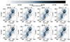 |
Fig. 6. Evolution of the coronal loops a, b, and c as seen in EM for plasma with at least 2 MK. Loop b contains most of the plasma. The sequence shows the beginning of the filling process of loop c between 08:44 UT and 08:46 UT. |
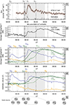 |
Fig. 7. Temporal evolution of the B1 flare of 6 June 2020 as seen in X-ray fluxes, average temperatures of sub-regions and timing of radio bursts. X-ray fluxes in the range 6 keV–7 keV are characterized by several peaks labeled with X0 to X2 (panel 1). The time axis was corrected for the light travel time. The timing of type-III bursts (dashed lines and panel 5) are shown in all panels. Radio bursts with fluxes above 10 SFU are displayed in bold line styles. Average temperatures of the AR based on the DEM reconstruction (panel 2). Temperature (panel 3) and EM evolution (panel 4) of the sub-regions (Fig. 5). |
3.4.1. First flare phase (08:40 UT–08:44 UT):
At the flare onset (Fig. 1) the foot points of loop A-B (connecting loop from western foot point of b to the region of loop a) lighten up (08:40:47 UT, 171 Å, a1). A Y-shaped structure emerges (171 Å, 08:40:47 UT, a1), with short-lasting EUV brightening at the two foot points of the structure and the foot point of loop A-B. The shape of loop a is similar to the pre-flare phase (e.g., at 08:35 UT). A major difference is the missing temperature increase. The restructuring activity continues and stops at 08:43 UT. The northern foot point of loop A-B is visible for one minute until it seems to be involved in some activity in loop a (cf. also Fig. 5).
The main energy release of the flare (related to X1) affects the loop-top and the western foot point of loop b (b1, 94 Å, 08:40:47 UT). Loop b is quickly heated (Tb1, temperature above 6 MK at 08:41 UT). Loop b is seen to be responsible for the rapid increase in X-ray radiation (Fig. 1), because it is the loop with the highest temperature and density. This is beneficial for the emission of soft X-ray radiation.
Loop c is further heated (Tc01, 08:38 UT–08:43 UT) with a heating rate of ≈0.5 MK/min at c-S (Fig. 7), while the heating rate in the middle part (c-mid) is only half of it in this period. c-mid is ≈1.5 MK cooler than the foot points at 08:43 UT. The foot point (c-S) reaches its maximum in temperature (in parts 6 MK) at 08:43 UT (Fig. 5). The temperature of c-S remains on this level for two minutes. The heating rate of c-mid decreases only slightly at 08:43 UT. The EM in the two parts of the loop is changing with very different pace. From 08:38 UT to 08:43 UT the EM of c-S rises by 30%, in the middle part of the loop the increase is about 5% (Fig. 7).
At the western part of loop b, a small enhancement appears (c1 in Fig. 4, 08:41:59 UT), which is orientated toward loop c and is located at the boundary of positive and negative polarity (Fig. 2, HMI). It could be related to a foot point of a loop connected to c-S. During the appearance of c1 the temperature Tb12 decreases with a higher pace, after 08:43 UT the cooling rate in loop b is rather stable at ≈0.1 MK/min. At 08:43:47 UT a similar structure as b01 reappears in loop b, two bright spots are seen in 171 Å (b2). At 08:44:47 UT b2 is seen again. This time it appears together with the neighboring northern foot point of loop c (c-N).
Second flare phase (08:44 UT–08:50 UT): The X-ray emission X2 is followed by a strong thermal response of the AR (full FOV temperature, Fig. 7). An overall temperature rise is not equally shared by the different sub-regions though. Most EM is still found in the dense and heated loop b; thus, the overall spatial distribution of EM has not changed much from the pre-flare phase to the second flare phase (Fig. 6).
Loop c brightens significantly in 94 Å, after previous enhancements in c-N and the western part of loop b at 08:45:11 UT in (171 Å). This trend continues and loop c dominates the appearance of the AR (94 Å) in the following minutes. The EM in c-mid increases by 30% from 08:44 UT to 08:48 UT (c2, Fig. 7). This happens at a time when c-S has already reached its maximum EM (concluded chromospheric evaporation). Despite noticeably higher EM, the densities in loop c (by assuming a similar extension along the line of sight) remain lower than in loop b. Considering the large volume of c there is a great amount of plasma needed to produce the observed increase, whereas c-S and b stay at their 08:44 UT levels (Fig. 7). An increasing width, doubled from 08:45 UT to 08:50 UT, leads to an extended volume of c at the end of the second flare phase.
At 08:45:11 UT the southern spot in loop b, b2, is the brightest region in the 171 Å image, in the following minutes it stays bright together with c-N. However, loop b is neither heated nor filled with more plasma after the energy release X2 (Fig. 7). The thermal response of X2 is only seen in loop c (Tc2). As a response to the foot point heating, the EM in c-mid increases (c2, Figs. 6 and 7). At the same time appears a sub-loop, c-S’, close to c-S (Fig. 5, 08:45:11 UT).
Gradual phase (08:50 UT–09:01 UT): After 08:49:24 UT loop A-B brightens and also the set of small loops below it show varying emission around 08:50 UT (171 Å). The EM increases (ag, 08:50 UT–08:51 UT), the temperature Tag increases one minute later as soon as the EM in loop a stagnates (Fig. 7). From 08:52:00 UT to 08:54:30 UT further activity at the northern foot point of loop A-B is observed (ag). As soon as the activity below loop A-B abruptly stops at 08:52:36 UT, there are spatially concentrated three bright points in the images. They appear close to the western foot point of loop A-B and move in two separated parts of loop b toward loop c. Simultaneously there is a bright structure in loop a, moving from north to south toward loop c. Timing and position of these spots suggest a secondary response, to the activity in loop A-B.
At 08:52:47 UT also the foot points of a sub-loop, b’, which is spatially framed by loop b, are illuminated in 171 Å (Fig. 4). The thermal response (Tag, Fig. 7) happens directly in the small loop connecting the foot points (Tbg). The temperature increases from 3 MK to 4 MK in the temperature maps (Fig. 5).
In the time after 08:55 UT new activity in the north-western edge of the AR becomes important. There is a small structure, λ, visible in 171 Å (Fig. 4, 08:58:24 UT), which magnifies and is visible as a line in north-south direction at 08:56:35 (Fig. 4). In the following minutes we observe the λ-shaped structure at the same position. Temperatures increase in this region, but it is not flare-related anymore. We stop the observations at 09:01 UT.
3.5. Dynamic radio spectroscopy of flare-accelerated electrons
During the event several type-III bursts (drift rates from −2 MHz/s to −5 MHz/s) appear in the dynamic radio spectra recorded by LOFAR (Fig. 8, Table A.3). We also discuss them separately for each flare phase (Fig. 1).
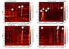 |
Fig. 8. Dynamic radio spectra recorded by LOFAR in the LBA. Solar type-III radio bursts of the pre-flare, first, second, and gradual flare phase are visible as increased flux densities with negative frequency drift. |
Additionally, the dynamic radio imaging spectroscopy reveals detailed information about the propagation of flare-accelerated electrons in the various flare phases. For each burst and frequency (Figs. 9, 10) the source position and propagation angle is determined. The position of the AR on the solar disk is marked with a gray circle in these figures. All radio source positions are in the south-eastern part of the field of view and are correlated in time with the other flare observations. Therefore, it is assumed, that the bursts are associated with the observed AR in the south.
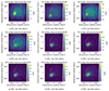 |
Fig. 9. Type-III radio source positions for R10 to R505 (flare phases are noted in the sub-captions). Contours are overplotted at the full width at half maximum of the radio maps. The colors of the contours correspond to their frequency, namely 80 MHz (purple), 70 MHz (blue), 60 MHz (green), 50 MHz (orange) and 40 MHz (red). The gray lines are the lines of longitude and latitude of the AR. |
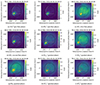 |
Fig. 10. Type-III radio source positions for burst R506 to R7g2 (flare phases are noted in the sub-captions). The colors of the contours correspond to their frequency, namely 80 MHz (purple), 70 MHz (blue), 60 MHz (green), 50 MHz (orange) and 40 MHz (red). The gray lines are the lines of longitude and latitude of the AR. |
Pre-flare phase (08:30 UT–08:40 UT): The first radio bursts (R10, R20, R30), which we consider to be related to the event are visible in the low band more than four minutes before the flare onset between 08:32 UT and 08:36 UT. Electron beams responsible for the radio radiation of these bursts, follow field lines in north, west and north-west direction. Their starting position is close to the line of sight above the AR and changes slightly from north of the AR (R10) to south (R20) and back again to north (R30). The radio flux increases with time from 0.3 SFU (R10) to 2 SFU (R30). While these bursts share a few similarities, the differences in propagation direction suggests treating them as individual bursts, which cannot be grouped based on the radio observations.
The main group of type-III bursts in this flare event consisting of burst R40, R501 to R507, appearing between 08:38:28 UT and 08:40:13 UT (Fig. 8), that is, at the end of the pre-flare phase. These bursts are only seen at lower heights in the corona and are partly identified as J-bursts (R503, Fig. 8). In contrast to the previous bursts R10, R20, R30, only little variations of the source position are observed for bursts between 08:38:38 UT and 08:40:13 UT (Figs. 9, 10). All bursts (R501 to R507) start at the eastern side of the AR and most of them propagate with propagation directions between 315° and 330° toward the other AR in the north. An exception is the R40, it propagates along the line of sight.
First flare phase (08:40 UT–08:44 UT): With the flare onset at 08:40 UT (GOES X-ray fluxes) the radio flux of type-III bursts decreases and after 08:40:49 UT the radio bursts disappear completely. Hence, the only burst in the first flare phase is R21 at 08:40:49 UT. R21 differs in many ways from the bursts between 08:38 UT and 08:40:13 UT, especially with respect to its propagation angle (W-directed), large source size and low radio flux.
Second flare phase (08:44 UT–08:50 UT): After the radio quiet period (08:40:49 UT–08:45:09 UT) and with the second impulsive increase in X-ray radiation (08:44 UT) a single burst (R52) with high fluxes is observed at 08:45:09 UT. R52 reaches fluxes of 30 SFU making it the strongest burst of the flare event. Notably, R52 shares many characteristics with the bursts R501 to R507. Propagation path, high radio flux and starting position are very similar although the bursts belong to different flare phases. A difference is that the source position of R52 changes strongly from 50 MHz to 40 MHz.
Gradual phase (08:50 UT–09:01 UT): Bursts observed in the gradual phase (Figs. 10e–10i) are characterized by emission across a broad frequency range. This suggest that they are produced by electrons propagating either on very far-reaching field lines or on open field lines. Burst R1g1 (08:51:32 UT) is for example seen in high altitudes of the solar atmosphere from frequencies of 23 MHz (≈0.9 RS). The bursts start position (at 80 MHz) is also closer to the AR. With 20 SFU R1g1 is one of the strongest bursts of the event. The propagation is similar to burst R10, but the two bursts have a different starting position. A second burst of similar shape is observed at 08:54:50 UT (R1g2). R1g2 has a minor maximum originating from the quiet Sun background.
Further bursts (R6g, R7g1, R7g2) in the gradual flare phase have in general low fluxes (below 1 SFU). They are included in the analysis to show, that the radio quiet period between 08:41 UT and 08:45 UT cannot be explained by a too low sensitivity of the LOFAR instrument since even bursts below 0.4 SFU are detected. Furthermore, they contain information about the magnetic connectivity after the flare. R6g propagates close to the line of sight in the LOFAR observations and slightly to the east for higher frequencies. The trajectory differs from the other bursts. R7g1 and R7g2 propagate in the same direction.
Trajectories of radio bursts and the PFSS model: A comparison with the PFSS model shows (Fig. 11), that most of the bursts follow field lines directed toward the other AR. One main path is taken by the flare-accelerated electrons responsible for these bursts, namely from the AR to the north-western direction away from the Sun with a maximal height level of 40 MHz (≈0.7 RS, Fig. 11). Since these field lines are orientated along the line of sight in lower heights and north-west orientated in their maximal height above the solar disk, the radio source positions at higher frequencies are shifted.
Bursts with northward trajectories (R10, R1g1, R1g2) follow field lines from the AR to the north pole (Fig. 11). Bursts with trajectories in purely west or east direction (R20, R21, R6g) are likely produced by electrons following large-scale loops surrounding the M loops in greater heights. These loops are visible in Fig. 2 (AIA 171 Å).
We summarize that the radio observations are in agreement with the PFSS model (Figs. 3, 11) and with the visible loops in the AIA data presented in the previous sections.
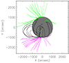 |
Fig. 11. Position of radio sources for burst R503 at four frequencies: 80 MHz (purple), 70 MHz (blue), 60 MHz (green), and 50 MHz (yellow) observed by LOFAR. The green and purple field lines are open; black field lines are closed. The field lines from the PFSS model are based on HMI/SDO data (displayed as gray surface of the Sun). The flare-accelerated electrons propagate along closed magnetic field lines in that example. |
3.6. Section summary
The emission by heated flare loops and by downward particle acceleration lead to the X-ray peaks in STIX and GOES observations at 08:31 UT, 08:39 UT, 08:41 UT, and 08:45 UT. As seen from the AIA observations and their extended analysis with a DEM reconstruction, the X-ray peaks are a consequence of triggered energy releases in the small-scale loop system of the AR. These changes are best resolved in 171 Å. Several impulsive energy releases (emission at foot points) are timely correlated with thermal responses in the time thereafter (Fig. 7).
We found characteristic EUV features in 171 Å, which are reappearing over the flare process. For loop b these are b0 (08:31 UT), b1 (08:40 UT) and bg (08:52:35 UT). Sinking temperatures during X2 show, that loop b is not contributing to the second flare peak. Loop a shows activity with a0 (08:33 UT–08:34 UT), a1 (08:40:47 UT), ag (08:40:47 UT–08:53:58 UT). The evolution of loop c consists of two temperature increases, Tc01 (08:38:30 UT–08:43:30 UT) and Tc2 (08:44:30 UT–08:48:00 UT).
Whether there is also upward-directed particle acceleration in combination with an open access to the higher corona during the heating periods of the AR is investigated with radio observations (LOFAR). Each radio burst has in principle its own characteristics and is in this sense unique. However, similarities in frequency range, trajectory or time of occurrence suggest a relation between selected bursts. During the pre-flare peak (X0’, 08:39 UT) and the second flare peak (X2, 08:45 UT), very similar bursts are observed (R501 to R507). Periods with no significant radio bursts are observed between X1 and X2 (08:40:13 UT–08:45:09 UT), and after the second flare peak (08:45:09 UT–08:51:32 UT).
4. Correlations in the multi-wavelength analysis
Here we discuss correlations in the temperature evolution, X-ray fluxes and the radio observations, which are presented separately in the previous section.
4.1. Sources of X-ray emission in the active region
Increased X-ray fluxes (X0, X0’, X1, X2) arise from the coronal loops in the AR as a consequence of magnetic reconnection and the reconfiguration of field lines. The DEM analysis allows the main loops responsible for the X-ray radiation in each flare phase to be identified.
We observed that X0 is correlated with loop b. This loop has the highest EM and temperatures during X0 and several minutes before and after it (Fig. 7, panel 3/4). Furthermore, GOES X-ray flux (Fig. 1) and EM evolution (Fig. 7) have a very similar shape. As for X0’, it is most likely emitted from the foot points of loop c. It is well correlated in time with the start of the gradual heating of loop c (Fig. 7). The heating rate in the foot point of loop c after X0’ is unchanged, the X-ray peak marks the onset of this heating process. The higher X-ray fluxes from 08:38 UT to 08:39 UT are not very correlated with loop b. Loop b is already slightly heated from 08:37 UT to 08:38 UT and keeps its temperature, while its EM decreases during X0’. At this point, the average temperatures are unchanged, and the temperatures and EM of c-mid have not yet increased either. These are indications of a non-thermal origin of X0’ related to the foot points of loop c.
The strongest X-ray peak in this event is X1, and it is correlated with the heating of loop b. As seen from the DEM analysis, loop b contains most of the heated plasma between 08:40 UT and 08:42 UT.
In the second flare phase, rising X-ray fluxes are accompanied by the simultaneously occurring EM-increase (c2) in loop c. At the peak X2 and in the following minute the heating rate in c-mid is increased (Fig. 7, Tc2). In EUV (Fig. 4, 08:45:11 UT) c-north shows also higher intensities. The different thermal evolution of loop b (cooling phase) and loop c (heating phase) after X2 suggest, that X2 is related to the energy release in loop c.
Further energy releases, which are not accompanied by X-ray radiation, are related to the loop a and loop A-B. These lead to increased EM between 08:32:30 UT and 08:33:30 UT and around 08:41 UT. Heating of the foot points of loop A-B is observed in the period 08:51 UT to 08:56 UT. There is also another sub-loop of loop b forming from 08:52:35 UT to 08:55 UT, also in this case there are no notable X-ray peaks in STIX or GOES (1 Å − 8 Å), but it is visible in the DEM maps with temperatures of 4 MK.
4.2. Relating radio bursts to the energy releases in the AR
Radio bursts are the result of an acceleration process in a certain region and its magnetic connectivity to the height where they can be detected. Both conditions need to be unchanged in order to produce bursts with the same characteristics.
The observed drift rates of −2 MHz/s–−5 MHz/s indicate radial kinetic energies of approximately 1 keV–3 keV (1.3 ⋅ 107 m/s–2.3 ⋅ 107 m/s), depending on the used density model (e.g., Newkirk 1961). A comparison of different density models is presented for example in Dabrowski et al. (2021). As shown by Mann et al. (1999),
![Mathematical equation: $$ \begin{aligned} f_{\rm pe}(r) = f_{\rm S} \cdot \exp \left[6.915 \cdot \left(\frac{R_{\rm S}}{r}-1\right)\right] \end{aligned} $$](/articles/aa/full_html/2025/02/aa49289-24/aa49289-24-eq3.gif) (3)
(3)
can be used as an appropriate approximation of regions with radial distances of r = 1.1 RS–3 RS (from the center of the Sun) with a surface density NS = 5.14 ⋅ 109 cm−3, and surface frequency fS = 644 MHz. The expression is based on the Newkirk model (Newkirk 1961) with a temperature of 1 ⋅ 106 K. 70 MHz corresponds to a height of 0.5 RS, 20 MHz corresponds to 1.0 RS above the solar surface. If the acceleration region is close to the loops seen in EUV observations, flare-accelerated electrons need to propagate about half a solar radius in radial direction before they are detected by LOFAR (LBA) at 70 MHz. This causes a delay of 14 s − 25 s between triggered acceleration and detection, for electrons with an average kinetic energy of 1 keV–3 keV.
Considering the electron travel time allows the present processes in the AR in the moment of particle acceleration to be determined. These processes could also be linked to the particle acceleration process, which is discussed in the interpretation section. Here we concentrate on the relations between the energy releases related to X0, X0’, X1, X2, and the radio bursts. There are also radio bursts without X-ray counterpart, these are covered in the end of the section.
In the early pre-flare phase, electrons responsible for R10 were accelerated in lower heights around 08:32:04 UT (assumed trigger time). At this time the heating of loop b is already completed. Loop a starts its activity and reaches an EM peak at 08:33:30 UT. During the trigger time of R20 (08:34:18 UT) loop a is already filled with more plasma (Fig. 7, 4) and small temperature increases happen along the loop (Fig. 6). After the burst the activity is concluded and the EM sinks. R30 (08:35:23 UT) occurs after the activity of loop a and cannot be linked to any activity during this time.
In the late pre-flare phase, R40 is triggered at 08:38:08, that is right at the onset of the heating process of loop c (Fig. 7, 4) and the onset of X0’ (Fig. 7, 1). The enhanced STIX flux (08:38:30 UT–08:39:30 UT) is correlated in time with the trigger times of radio bursts R40 and R501–R507 (08:38:08 UT–08:39:53 UT). In the rising flux phase (08:38:30 UT–08:39:00 UT) of the X-ray observations radio bursts with higher fluxes (up to 25 SFU) are observed.
In the first flare phase, R21 occurs and is characterized by rather low fluxes below 1 SFU. The estimated trigger time of R21 is 08:40:19 UT. During this time loop b is reaching the maximal heating rate and is filled rapidly with hot plasma. That is, in the middle of the first major heating process of the AR (Fig. 7, 2). The heating rate of loop c is not changed after this burst, but the EM rises in the box for loop a (Fig. 7, 4) and loop A-B appears at the same time in AIA 94 Å (Fig. 4). R21 is timely correlated with the heating of loop b and the formation of loop A-B.
In the second flare phase, R52 is triggered around 08:44:59 UT. At this time the X-ray flux is rising and has almost reached X2. Loop c has reached a constant temperature at c-S and is still heated with the same heating rate at c-mid (Fig. 7). With the triggering of R52 the heating rate of c-mid is increased. Also, the EM increases stronger in the minutes after the burst. R52 is therefore correlated in time with X2, which is seen to be emitted by loop c (Sect. 4.1).
In the gradual flare phase, R1g1 is triggered around 08:51:12 UT. Loop b and loop c are in the cooling phase at this time. Loop A-B is in the beginning of a heating process at 08:51:30 UT, which lasts from 08:51:30 UT to 08:53:30 UT. The timing of R1g1 is correlated with the activity in loop A-B (Tag, Fig. 7). At the end of Tag burst R1g2 is triggered (08:54:30 UT). Already 95 seconds before, at 08:52:55 UT, there is an energy release in loop b (Fig. 4) and the thermal response becomes visible at 08:54:00 UT in the average temperatures (Tbg, Fig. 7, 3). R1g2 is more correlated with the evolution of loop A-B.
R6g, R7g1 and R7g2 are triggered around 08:59:28 UT, 08:59:30 UT, 09:00:58 UT. At this time there is no relevant activity in the loops a, b, A-B, but the λ-shaped structure is active in the north-western part of the AR. The bursts are related in time with this structure, which is located closer to the large-scale magnetic field of the AR.
The strongest correlation between radio bursts and energy releases in the AR is found for X0’ and X2. These bursts (R40, R501–R507 and R52) are related to the energy release in loop c and have a reduced frequency range of 85 MHz–48 MHz, in comparison to other bursts with 85 MHz–30 MHz (corresponding to heights up to 0.8 RS). The J-shape of burst R503 and a stopping frequency in the range of 65 MHz–48 MHz for bursts in the late pre-flare phase (corresponding to heights of 0.5 RS–0.6 RS), indicate that the radio emission originates from lower regions in the solar atmosphere, thus providing evidence for injection of electrons into smaller large-scale loops during this time (L loop in Fig. 3).
4.3. Relating heating periods and radio burst fluxes
As seen from Sect. 4.2, the radio bursts appear mainly at the beginning or end of heating periods in this event. The period in between, either impulsive or gradual heating, is not accompanied by type-III bursts in these observations. An example is the heating of c-mid (08:39:00 UT–08:45:00 UT) and the radio quiet time after R507 (triggered at 08:40:19 UT). In the period of about five minutes after this energy input, the heating rate remains. In the second flare phase the same duration of effect is observed for R52 (08:44:59 UT) and the temperature increase with a maximum at 08:50 UT.
There are also indications for loop heating without any related radio bursts. The radio bursts are correlated with major changes in EM and temperature of loop a, A-B and c, or formation of the λ-structure (Sect. 4.2).
There are no indications of radio bursts linked to the evolution of loop b in the pre-flare phase (Tb0), main flare phase (Tb1), or in the gradual phase (Tbg). This is quite notable because closer to the main STIX X-ray peaks (X0 and X1) and the main heating phase, much more energy for particle acceleration should be available. The absence can either be a result of missing particle acceleration or a closed magnetic field configuration, which leads to an interrupted magnetic connectivity and forces the flare-accelerated electrons to remain in the AR.
We have investigated the evolution of particle acceleration, loops affected by the energy release and the trajectories of flare-accelerated electrons observed above the AR. In the next section we interpret the findings and discuss the possible influence of the magnetic connectivity on the presented flare observations.
5. Interpretation
In this section we aim to explain why radio observations in this event are on the one hand well-correlated with changes of the flaring loops in the AR, but are on the other hand absent during certain energy releases in the low corona. On that account possible magnetic reconnection processes and the evolution of the magnetic connectivity are discussed as possible explanations for presence and absence (i.e., the modulation) of type-III bursts during certain flare phases. Finally, the findings are compared with selected previous studies.
5.1. Magnetic reconnection in the active region
The presented observations suggest that the loops of the AR are interacting by magnetic reconnection. Possible interactions based on the photospheric magnetic field data are summarized in Fig. 12. The result would be a shortening of the total loop length and a reduction of stored energy. In the AIA observations not all loops of the AR are filled with plasma, so that this is only an extract of the main loops. The sketches illustrate how loop A-B could be formed from loop a and b by a reconnection process. Observational evidence for this process is found for example in the AIA 171 Å data at 08:41:59 UT (Fig. 4, easternmost red dot). If loop A-B was formed in this way, it would reduce the magnetic flux in loop b.
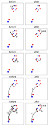 |
Fig. 12. Possible transition of loops due to magnetic reconnection. The polarities are based on the HMI data. Regions with positive polarity (blue) and negative polarity (red) are connected by magnetic field lines. These processes can also take place simultaneously. The bottom panel shows a superposition of all the loops above. |
The structural evolution of loop b, in which it changes from a J-shaped structure toward a semicircle (Fig. 4, 94 Å) is likely a result of successive magnetic reconnection of the sub-loops of loop b (e.g., Yang et al. 2023). In Fig. 12 we show the opposite case, in which the loop length is reduced by reconnecting two closed current-carrying loops with each other, as described in the flare model by Melrose (1997).
Loop c is of particular importance in the flare event and its evolution is well correlated with the radio bursts. A polarity inversion close to the positive polarity of loop b is responsible for a number of possible reconnection processes. In the sketched case, an interaction with a sub-loop of loop b is shown. Such a process could support the speeded heating of loop c after 08:45 UT. The sketch is in agreement with Fig. 5 (08:45:11 UT and 08:46:11 UT), where a temperature increase happens at the same position as the newly formed small loop in the sketch.
At c-S there is also a region of negative polarity. We see in the AIA observations thin loops with similar shape as loop c, but with inverted orientation (HMI data, Fig. 2) and filled with much cooler plasma. When comparing the panels of Fig. 5 between 08:43:11 UT and 08:55:11 UT, there is always a gap in the otherwise uniform temperatures along loop c, where we expect the crossing of both loops as seen from the given observing angle. A magnetic reconnection between those two could explain the heated loop close to c-S at 08:45:11 UT in Fig. 5.
A combination of the discussed processes is likely occurring in the flare event. There are energy build-up phases (08:35 UT–08:40 UT for loop b, Fig. 7, 2) and energy release phases (08:40 UT–08:41 UT for loop b) triggered by magnetic reconnection. The rapid changes of field lines can lead to particle acceleration. How the particles are exactly accelerated in these scenarios is beyond the scope of this paper. We only assume here, that each of these reconnection processes is leading to a specific acceleration process (also, when triggered more than once). The location of the acceleration region is expected to be close to the heated flare loops of the AR.
5.2. Magnetic connectivity
We have identified their energy release sites in the AR, mainly the three loops, a connecting loop (A-B) and several sub-loops. We assume a symmetric acceleration process in which particles are accelerated upward and downward.
Type-III bursts correlated in time with these energy releases in neighboring loops, are emitted along similar propagation trajectories. That is also the case for bursts occurring in different flare phases as long they are associated with the same loop in the AR. Each of the related particle acceleration regions seems to have a different magnetic connectivity to the higher corona. Bursts triggered more than once (e.g., R501 to R507) likely originate from the same acceleration region and process. The missing bursts related to loop b are probably a result of the magnetic reconnection type (from closed to closed). The large-scale magnetic field, consisting of encapsulated loop systems, is very stable and not affected by the flare in contrast to the magnetic connectivity. Once flare-accelerated electrons can leave the AR and lower coronal heights, they tend to end up on very similar large-scale magnetic field lines. This can be seen from the pairs and groups of radio bursts in Fig. 7 (panel 5).
Heating and magnetic connectivity are anticorrelated in a sense, that loops with good magnetic connectivity have lower heating rates (slope of Tag < Tc01), while the strongest temperature increases were observed in loop b (Tb1) characterized by a suppressed magnetic connectivity.
5.3. Comparison with previous studies
This paper stands in context with several other studies, which focused on the relative timing of hard X-ray, microwave and lower frequency radio bursts in different phases of flares (Trottet 1986) and partly also on their relation to the small- and large-scale magnetic fields in the low, middle and upper corona (Trottet 2003; Trottet et al. 2006). Major results supporting the interpretation of data given in this paper are that hard X-ray radiation and radio emitting electrons are produced at common acceleration sites (Trottet 2003). That is based on comparisons of radio emission below ≈410 MHz and X-rays above 50 keV (Vilmer et al. 2002; James & Vilmer 2023).
By choosing a small B-class flare, the findings for relations between X-rays and radio observations above 150 MHz are extended to emission of radiation with lower frequencies (i.e., for greater solar heights more relevant for space weather). It was shown for the flare event on 6 June 2020, that the latest DEM reconstruction codes allow energy release sides with high spatial resolution to be identified, although there are no hard X-ray images available for the event. The heating onset times are as important in this event as the hard X-ray peaks in other stronger events.
In contrast to previous studies by Trottet et al. (2006), who found that the source position at a given frequency changes from burst to burst for each of the five observing frequencies above 164 MHz, R40 to R503, and R506 are examples for bursts with the same source positions for frequencies 60 MHz–80 MHz in the flare event on 6 June 2020. Additionally, a burst with similar trajectory is observed five minutes later in the gradual flare phase (R52). These radio sources propagate along large-scale magnetic loops from one AR to the other AR present in the north-west (similar as in Nakajima et al. 1984).
In agreement with the findings from other much stronger events (e.g., Chupp et al. 1993; Trottet et al. 1994; Trottet 2003), the B-class flare starts with an acceleration process before the impulsive phase in loop b. The particle acceleration is correlated with a gradual heating process in a neighboring loop, which starts before the heating of loop b. Type-III bursts appear about one minute (similar to Chupp et al. 1993) earlier before the initiation of the main X-ray peak. The source of type-III bursts are likely rapid changes in the topology of the magnetic field as a consequence of interacting loops as suggested already in Chupp et al. (1993). With the DEM reconstruction, we provide further information about the evolving loops and their expected magnetic connectivity (Fig. 12).
Radio emission at the relevant frequencies are clear signs that flare-accelerated particles have access to the higher corona (Klein et al. 2010). In other events, as 5 November 1998, with a similar PFSS magnetic field configuration of loops with different sizes and strong indications for a joint accelerator for hard X-ray radiation and radio emitting electrons, there was no evidence for a direct magnetic connection between the hard X-ray emitting structures and the radio sources (Trottet et al. 2006). That raises questions regarding the trajectory of electrons from the acceleration region close to the heated flare loops to the large-scale magnetic arches.
For the larger coronal heights studied here, the observed trajectories are rather close to the line of sight (Figs. 9, 10), although the particles must propagate through the overlaying mid-scale loops (M loops, Fig. 2). Hints for an influence of these larger loops on the particle trajectories is only seen from the missing south-east trajectories in the burst observations, otherwise we did not find any observational evidence for their influence. That is in agreement with detailed observations of trajectories from the AR to the middle corona, indicating that the corona is rather permeable in nature, consisting of many unresolved tracks, furthermore the type-III emitting strands were found to have a direct connectivity to the reconnection region (Chen et al. 2013). This further supports our interpretation, that the access to the higher corona depends mainly on the magnetic connectivity of the small-scale core loops in the low corona, while the other parts of the encapsulated loop systems in greater heights were found to be rather stable.
6. Conclusion
In this paper, we have investigated the propagation of flare-accelerated electrons, coronal loop heating, and the underlying magnetic connectivity of lower (< 40 Mm = 0.057 RS height) and higher corona (0.4 RS–1.0 RS height) for different flare phases. Our aim was to explore the possible influences of magnetic connectivity on the evolution of the flare process, the relative timing of multi-wavelength observations, and the modulation of type-III radio bursts between 20 MHz and 85 MHz.
To this end, we conducted a case study of a B1 solar flare event from 08:30 UT to 09:01 UT on 6 June 2020. The advantages of studying this small event are a rather simple sub-structure, no saturation effects in the DEM analysis, and negligible pre-heating of plasma due to earlier activity. This allowed us to study the magnetic connectivity while the main aspects of the general flare setup remained rather constant. By applying a detailed DEM reconstruction of the AIA/EUV observations, it was possible to identify single loops in the low corona, which are the source of the thermal flare emission. The traces of flare-accelerated electrons, type-III radio bursts, were investigated with a spectroscopic solar dynamic radio imager (LOFAR). The type-III bursts are emitted in the higher corona close to the AR when the sources are projected to the solar surface from the LOFAR perspective. The propagation paths of the flare-accelerated electrons producing the radio bursts are in agreement with information about the magnetic field from the PFSS model and AIA observations. The spatial agreement of EUV and LOFAR observations suggest that the observed regions in different heights of the solar atmosphere are in principal magnetically connected.
Electron travel times of approximately 14 s–25 s were found based on a density model and the observed frequency drifts of radio bursts. We searched for any indication of primary energy release in the loops around the estimated electron acceleration time (e.g., foot point heating) and their thermal response in the time thereafter as seen from the DEM map analysis. With this method, we found evidence for a linkage of certain acceleration processes, particle trajectories, and the heating of three core loops in the AR. This is also the case for bursts occurring in different flare phases, as long as they are associated with the same loop in the AR. In these cases, the bursts are emitted along similar trajectories. The onset of selected heating processes in the core loops are correlated in time with type-III bursts. Heating processes, lasting up to five minutes after the conclusion of type-III radio emission, continue as radio quiet. In some cases, as for the main flare loop, there are no associated radio bursts detected between 20 MHz and 85 MHz in the whole event.
Our aim was to explain why radio observations in this event are on the one hand well correlated with changes of the flaring loops in the AR but are on the other hand absent during the main energy release and during the continuation of selected heating processes in the low corona. If the acceleration process is symmetric (i.e., electrons are accelerated toward and away from the Sun), we consider that access to the higher corona is suppressed, during an ongoing heating process as a thermal response to the downward-accelerated particles. No particular changes have been observed in the EUV data of the mid-scale magnetic field systems (loop length ≈2 ⋅ 102 Mm). Also, the large-scale field as seen from trajectories of radio sources was rather stable across the different flare phases. Once the particles leave the AR, they tend to end up on very similar large-scale magnetic field lines. Hence, we consider the influence of the mid- and large-scale magnetic fields on the reduced magnetic connectivity to be small here, and we assume that the access to the higher corona is already suppressed in the low corona.
We separated the superposition of two heating processes in different but neighboring loops by applying the multi-wavelength analysis. The occurrence of type-III bursts before the onset of X-rays (originating from the smaller loop) is interpreted as a consequence of the poor magnetic connectivity during the loop-loop interaction of the main flare. However, it is likely that the energy releases are related. This would imply an interaction between a longer loop with good connection to the higher corona and a system of short loops with strong heating and poor upward connection. We suggest suppressed access to the higher corona in the core loops of the AR, leading to more effective heating and absent type-III radio bursts between 20 MHz and 85 MHz, as a possible explanation for the asymmetric evolution in the lower and higher corona.
There are slight indications of an anticorrelation of heating and magnetic connectivity in a sense that loops with good magnetic connectivity (i.e., loops with associated type-III bursts) have lower heating rates in this event, while the strongest temperature increases are observed in small loops with poor magnetic connectivity. We also found signs of the continuation of selected heating processes with closed magnetic connectivity to the higher corona. However, observations of the complete electron trajectories (including microwave observations) would be needed to ensure this for heights below 0.4 RS.
Since other flare events originate from ARs with more complex loop systems, it is conceivable that coronal loops with very different magnetic connectivity exist in such regions as well. Scenarios in which the type-III bursts occur before the X-ray peak could be partly due to the phenomenon assumed here: an interaction of coronal loops with good and poor magnetic field connection.
In the future, the presented multi-wavelength analysis could be applied to a set of slightly stronger events originating from similar ARs with stable large-scale magnetic field. This may further support the influence of the magnetic connectivity on the evolution of coronal loops and the propagation of flare-accelerated electrons.
Data availability
Movie associated to Fig. 4 is available at https://www.aanda.org
Acknowledgments
We thank the Deutsche Forschungsgemeinschaft (DFG, German Research Foundation) and the National Science Centre, Poland, for granting “LOFAR observations of the solar corona during Parker Solar Probe perihelion passages” in the Beethoven Classic 3 funding initiative under project numbers VO 2123/1-1 and 2018/31/G/ST9/01341, respectively. UWM would like to thank the Ministry of Education and Science of Poland for granting funds for the Polish contribution to the International LOFAR Telescope, LOFAR2.0 upgrade (decision number: 2021/WK/2) and for maintenance of the LOFAR PL-612 Bałdy station (decision number: 28/530020/SPUB/SP/2022). This paper is based (in part) on data obtained with the International LOFAR Telescope (ILT) under project code LT16_001. LOFAR (van Haarlem et al. 2013) is the Low Frequency Array designed and constructed by ASTRON. It has observing, data processing, and data storage facilities in several countries, that are owned by various parties (each with their own funding sources), and that are collectively operated by the ILT foundation under a joint scientific policy. The ILT resources have benefitted from the following recent major funding sources: CNRS-INSU, Observatoire de Paris and Université d’Orléans, France; BMBF, MIWF-NRW, MPG, Germany; Science Foundation Ireland (SFI), Department of Business, Enterprise and Innovation (DBEI), Ireland; NWO, The Netherlands; The Science and Technology Facilities Council, UK; Ministry of Science and Higher Education, Poland. This research is based on observations made with AIA and HMI on NASA’s SDO satellite and with STIX on the Solar Orbiter satellite. Solar Orbiter is a mission of international cooperation between ESA and NASA, operated by ESA. We acknowledge the Joint Science Operations Center (JSOC) for providing the SDO data. Software: DEM sparse inversion code (Su et al. 2018). PFSS Model as part of the SolarSoftWare (SSW, Freeland & Handy 1998; Schrijver et al. 2003). This research used version 4.0.6 of the SunPy open source software package (The SunPy Community 2020).
References
- Aschwanden, M. J. 2004, Physics of the Solar Corona. An Introduction (Praxis Publishing Ltd) [Google Scholar]
- Benz, A. O., Barrow, C. H., Dennis, B. R., et al. 1983, Sol. Phys., 83, 267 [NASA ADS] [CrossRef] [Google Scholar]
- Breitling, F., Mann, G., Vocks, C., Steinmetz, M., & Strassmeier, K. G. 2015, Astron. Comput., 13, 99 [NASA ADS] [CrossRef] [Google Scholar]
- Carmichael, H. 1964, NASA Spec. Publ., 50, 451 [NASA ADS] [Google Scholar]
- Caspi, A., Seaton, D., Casini, R., et al. 2023, BAAS, 55, 048 [Google Scholar]
- Chen, B., Bastian, T. S., White, S. M., et al. 2013, ApJ, 763, L21 [NASA ADS] [CrossRef] [Google Scholar]
- Cheung, M. C. M., Boerner, P., Schrijver, C. J., et al. 2015, ApJ, 807, 143 [Google Scholar]
- Chupp, E. L., Trottet, G., Marschhauser, H., et al. 1993, A&A, 275, 602 [NASA ADS] [Google Scholar]
- Dabrowski, B., Flisek, P., Mikuła, K., et al. 2021, Remote Sensing, 13, 148 [NASA ADS] [CrossRef] [Google Scholar]
- Dabrowski, B., Wolowska, A., Vocks, C., et al. 2025, Acta Geophys., 73, 987 [Google Scholar]
- Freeland, S. L., & Handy, B. N. 1998, Sol. Phys., 182, 497 [Google Scholar]
- Ginzburg, V. L., & Zhelezniakov, V. V. 1958, Soviet Astron., 2, 653 [NASA ADS] [Google Scholar]
- Handy, B. N., & Schrijver, C. J. 2001, ApJ, 547, 1100 [NASA ADS] [CrossRef] [Google Scholar]
- Harra, L., Brooks, D. H., Bale, S. D., et al. 2021, A&A, 650, A7 [NASA ADS] [CrossRef] [EDP Sciences] [Google Scholar]
- Heald, G., Bell, M. R., Horneffer, A., et al. 2011, JApA, 32, 589 [NASA ADS] [Google Scholar]
- Hirayama, T. 1974, Sol. Phys., 34, 323 [Google Scholar]
- James, T., & Vilmer, N. 2023, A&A, 673, A57 [NASA ADS] [CrossRef] [EDP Sciences] [Google Scholar]
- Kane, S. R. 1972, Sol. Phys., 27, 174 [NASA ADS] [CrossRef] [Google Scholar]
- Kane, S. R., Benz, A. O., & Treumann, R. A. 1982, ApJ, 263, 423 [NASA ADS] [CrossRef] [Google Scholar]
- Klein, K. L., Trottet, G., & Klassen, A. 2010, Sol. Phys., 263, 185 [NASA ADS] [CrossRef] [Google Scholar]
- Kopp, R. A., & Pneuman, G. W. 1976, Sol. Phys., 50, 85 [Google Scholar]
- Krucker, S., Kontar, E. P., Christe, S., & Lin, R. P. 2007, ApJ, 663, L109 [CrossRef] [Google Scholar]
- Krucker, S., Hurford, G. J., Grimm, O., et al. 2020, A&A, 642, A15 [NASA ADS] [CrossRef] [EDP Sciences] [Google Scholar]
- Kundu, M. R., Gergely, T. E., & Golub, L. 1980, ApJ, 236, L87 [NASA ADS] [CrossRef] [Google Scholar]
- Lemen, J. R., Title, A. M., Akin, D. J., et al. 2012, Sol. Phys., 275, 17 [Google Scholar]
- Lin, R. P. 1974, Space Sci. Rev., 16, 189 [NASA ADS] [CrossRef] [Google Scholar]
- Lin, R. P., Evans, L. G., & Fainberg, J. 1973, Astrophys. Lett., 14, 191 [NASA ADS] [Google Scholar]
- Mann, G., Jansen, F., MacDowall, R. J., Kaiser, M. L., & Stone, R. G. 1999, A&A, 348, 614 [NASA ADS] [Google Scholar]
- Mann, G., Breitling, F., Vocks, C., et al. 2018, A&A, 611, A57 [NASA ADS] [CrossRef] [EDP Sciences] [Google Scholar]
- Maxwell, A., & Swarup, G. 1958, Nature, 181, 36 [NASA ADS] [CrossRef] [Google Scholar]
- McMullin, J. P., Waters, B., Schiebel, D., Young, W., & Golap, K. 2007, in Astronomical Data Analysis Software and Systems XVI, eds. R. A. Shaw, F. Hill, & D. J. Bell, ASP Conf. Ser., 376, 127 [Google Scholar]
- Melrose, D. B. 1985, in Solar Radiophysics: Studies of Emission from the Sun at Metre Wavelengths, eds. D. J. McLean, & N. R. Labrum, 177 [Google Scholar]
- Melrose, D. B. 1997, ApJ, 486, 521 [NASA ADS] [CrossRef] [Google Scholar]
- Müller, D., St. Cyr, O. C., Zouganelis, I., et al. 2020, A&A, 642, A1 [Google Scholar]
- Nakajima, H., Dennis, B. R., Hoyng, P., et al. 1984, BAAS, 16, 524 [Google Scholar]
- Neupert, W. M. 1968, ApJ, 153, L59 [NASA ADS] [CrossRef] [Google Scholar]
- Newkirk, G. 1961, ApJ, 133, 983 [NASA ADS] [CrossRef] [Google Scholar]
- Raulin, J. P., Vilmer, N., Trottet, G., et al. 2000, in High Energy Solar Physics Workshop – Anticipating Hess!, eds. R. Ramaty, & N. Mandzhavidze, ASP Conf. Ser., 206, 245 [Google Scholar]
- Reid, H. A. S. 2020, Front. Astron. Space Sci., 7, 56 [NASA ADS] [CrossRef] [Google Scholar]
- Reid, H. A. S., & Kontar, E. P. 2021, Nat. Astron., 5, 796 [NASA ADS] [CrossRef] [Google Scholar]
- Reid, H. A. S., Vilmer, N., & Kontar, E. P. 2011, A&A, 529, A66 [NASA ADS] [CrossRef] [EDP Sciences] [Google Scholar]
- Schrijver, C. J., De Rosa, M. L., & Title, A. M. 2003, ApJ, 590, 493 [NASA ADS] [CrossRef] [Google Scholar]
- Sturrock, P. A., & Coppi, B. 1966, ApJ, 143, 3 [NASA ADS] [CrossRef] [Google Scholar]
- Su, Y., Veronig, A. M., Hannah, I. G., et al. 2018, ApJ, 856, L17 [NASA ADS] [CrossRef] [Google Scholar]
- The SunPy Community (Barnes, W. T., et al.) 2020, ApJ, 890, 68 [Google Scholar]
- Trottet, G. 1986, Sol. Phys., 104, 145 [NASA ADS] [CrossRef] [Google Scholar]
- Trottet, G. 2003, Adv. Space Res., 32, 2403 [Google Scholar]
- Trottet, G., Chupp, E. L., Marschhaeuser, H., et al. 1994, A&A, 288, 647 [NASA ADS] [Google Scholar]
- Trottet, G., Correia, E., Karlický, M., et al. 2006, Sol. Phys., 236, 75 [NASA ADS] [CrossRef] [Google Scholar]
- van Haarlem, M. P., Wise, M. W., Gunst, A. W., et al. 2013, A&A, 556, A2 [NASA ADS] [CrossRef] [EDP Sciences] [Google Scholar]
- Vilmer, N., Krucker, S., Lin, R. P., & The Rhessi Team 2002, Sol. Phys., 210, 261 [NASA ADS] [CrossRef] [Google Scholar]
- Wild, J. P. 1950, Aust. J. Sci. Res. A Phys. Sci., 3, 541 [NASA ADS] [Google Scholar]
- Yang, L., Yan, X., Xue, Z., et al. 2023, ApJ, 952, 43 [NASA ADS] [CrossRef] [Google Scholar]
- Zheleznyakov, V. V., & Zaitsev, V. V. 1970, Soviet Astron., 14, 250 [NASA ADS] [Google Scholar]
Appendix A: Tables
EUV features in the AR and their properties (cf. Fig. 4, attached movie).
Thermal features in the AR and their properties based on the DEM reconstruction (cf. Fig. 5, 7).
Type-III radio bursts and their properties (cf. Fig. 8, 9, 10). Radio bursts with fluxes above 10 SFU are highlighted in bold. The radio source position is noted with respect to the position of the AR, when the sources are projected to the solar surface from the LOFAR perspective. The propagation direction is in the same way the apparent movement on the solar disk with 0° as north, 180° as south, 90° as west and 270° as east.
All Tables
Thermal features in the AR and their properties based on the DEM reconstruction (cf. Fig. 5, 7).
Type-III radio bursts and their properties (cf. Fig. 8, 9, 10). Radio bursts with fluxes above 10 SFU are highlighted in bold. The radio source position is noted with respect to the position of the AR, when the sources are projected to the solar surface from the LOFAR perspective. The propagation direction is in the same way the apparent movement on the solar disk with 0° as north, 180° as south, 90° as west and 270° as east.
All Figures
|
Fig. 1. Smoothed GOES X-ray fluxes in 1 Å − 8 Å and 0.5 Å − 4 Å. Flare phases are marked with black vertical lines between the flare onset at 08:40 UT and the second flare onset at 08:44 UT and between the second flare onset and the peak X-ray flux at 08:47 UT. The dashed line highlights the onset of the main group of type-III radio bursts (08:38:30 UT–08:40 UT) at the end of the pre-flare phase. |
| In the text | |
|
Fig. 2. AIA observations in two channels and HMI data show the coronal loops of the AR with different sizes and magnetic polarities. Top panel: Magnetic field lines in channel 171 Å. Middle panel: Magnetic field lines in channel 94 Å. This channel shows mainly the small-scale loops of the AR. Larger loops with lower temperatures are only faintly visible. Bottom panel: Colorized magnetogram based on HMI data showing the different polarities of the AR. The overlaid illustrations of possible loops were identified by eye from the AIA observations. |
| In the text | |
|
Fig. 3. PFSS model for a starting height of 1.01 solar radii and a projection centroid of L0 = 100° and B0 = −30°. Displayed in green are data from channel 94 Å (AIA) to complement the model. |
| In the text | |
|
Fig. 4. AIA observations in 171 Å and 94 Å of the small-scale AR with the main loops a, b, c, and A-B. White circles indicate the foot points of the overlaying M and L loops (Fig. 2). Enhancements of intensities are marked with red dots and white boxes. These highlight foot points and loop-tops of the suddenly changing loops. Red arrows show the orientation of the loops based on the polarity of their foot points (HMI data, Fig. 2). The associated movie is available online. |
| In the text | |
|
Fig. 5. Evolution of the core loops of the AR as seen in the EM-weighted temperature maps. Changes and important structures are marked with white arrows. The influence of the flare on the AR can be especially seen at 08:41 UT (loop b reaches temperature of 7 MK in the first flare phase) and at 08:45 UT (loop c is strongly heated during the second impulsive flare phase). White boxes in the image at 08:46:11 UT are the sub-regions for the temperature analysis (Fig. 7). |
| In the text | |
|
Fig. 6. Evolution of the coronal loops a, b, and c as seen in EM for plasma with at least 2 MK. Loop b contains most of the plasma. The sequence shows the beginning of the filling process of loop c between 08:44 UT and 08:46 UT. |
| In the text | |
|
Fig. 7. Temporal evolution of the B1 flare of 6 June 2020 as seen in X-ray fluxes, average temperatures of sub-regions and timing of radio bursts. X-ray fluxes in the range 6 keV–7 keV are characterized by several peaks labeled with X0 to X2 (panel 1). The time axis was corrected for the light travel time. The timing of type-III bursts (dashed lines and panel 5) are shown in all panels. Radio bursts with fluxes above 10 SFU are displayed in bold line styles. Average temperatures of the AR based on the DEM reconstruction (panel 2). Temperature (panel 3) and EM evolution (panel 4) of the sub-regions (Fig. 5). |
| In the text | |
|
Fig. 8. Dynamic radio spectra recorded by LOFAR in the LBA. Solar type-III radio bursts of the pre-flare, first, second, and gradual flare phase are visible as increased flux densities with negative frequency drift. |
| In the text | |
|
Fig. 9. Type-III radio source positions for R10 to R505 (flare phases are noted in the sub-captions). Contours are overplotted at the full width at half maximum of the radio maps. The colors of the contours correspond to their frequency, namely 80 MHz (purple), 70 MHz (blue), 60 MHz (green), 50 MHz (orange) and 40 MHz (red). The gray lines are the lines of longitude and latitude of the AR. |
| In the text | |
|
Fig. 10. Type-III radio source positions for burst R506 to R7g2 (flare phases are noted in the sub-captions). The colors of the contours correspond to their frequency, namely 80 MHz (purple), 70 MHz (blue), 60 MHz (green), 50 MHz (orange) and 40 MHz (red). The gray lines are the lines of longitude and latitude of the AR. |
| In the text | |
|
Fig. 11. Position of radio sources for burst R503 at four frequencies: 80 MHz (purple), 70 MHz (blue), 60 MHz (green), and 50 MHz (yellow) observed by LOFAR. The green and purple field lines are open; black field lines are closed. The field lines from the PFSS model are based on HMI/SDO data (displayed as gray surface of the Sun). The flare-accelerated electrons propagate along closed magnetic field lines in that example. |
| In the text | |
|
Fig. 12. Possible transition of loops due to magnetic reconnection. The polarities are based on the HMI data. Regions with positive polarity (blue) and negative polarity (red) are connected by magnetic field lines. These processes can also take place simultaneously. The bottom panel shows a superposition of all the loops above. |
| In the text | |
Current usage metrics show cumulative count of Article Views (full-text article views including HTML views, PDF and ePub downloads, according to the available data) and Abstracts Views on Vision4Press platform.
Data correspond to usage on the plateform after 2015. The current usage metrics is available 48-96 hours after online publication and is updated daily on week days.
Initial download of the metrics may take a while.