| Issue |
A&A
Volume 694, February 2025
|
|
|---|---|---|
| Article Number | A130 | |
| Number of page(s) | 9 | |
| Section | Cosmology (including clusters of galaxies) | |
| DOI | https://doi.org/10.1051/0004-6361/202346891 | |
| Published online | 06 February 2025 | |
Are light curve classification metrics good proxies for SN Ia cosmological constraining power?
1
McWilliams Center for Cosmology, Department of Physics, Carnegie Mellon University,
Pittsburgh,
PA,
USA
2
Pittsburgh Particle Physics, Astrophysics, and Cosmology Center (PITT PACC), Physics and Astronomy Department, University of Pittsburgh,
3941 O’Hara St,
Pittsburgh,
PA
15260,
USA
3
SLAC National Accelerator Laboratory,
2575 Sand Hill Rd,
Menlo Park,
CA
94025,
USA
4
Université Clermont Auvergne, CNRS/IN2P3, LPC,
63000
Clermont-Ferrand,
France
5
CENTRA/COSTAR, Instituto Superior Técnico, Universidade de Lisboa,
Av. Rovisco Pais 1,
1049-001,
Lisboa,
Portugal
6
Independent Researcher,
Ingolstadt,
Germany
7
Donald Bren School of Information and Computer Sciences, University of California,
Irvine,
CA
92697,
USA
8
CENTRA/SIM, Faculdade de Ciências, Universidade de Lisboa,
Ed. C8, Campo Grande,
1749-016
Lisboa,
Portugal
9
Centre for Astrophysics Research, University of Hertfordshire,
College Lane,
Hatfield
AL10 9AB,
UK
10
Department of Computer Science, University of California Irvine,
Irvine,
CA,
USA
11
Physics Department, Brookhaven National Laboratory,
Upton,
NY
11973,
USA
12
Institute of Space Sciences (ICE, CSIC), Campus UAB, Carrer de Can Magrans, s/n,
08193
Barcelona,
Spain
13
Institut d’Estudis Espacials de Catalunya (IEEC),
08034
Barcelona,
Spain
★ Corresponding author; This email address is being protected from spambots. You need JavaScript enabled to view it.
Received:
12
May
2023
Accepted:
19
April
2024
Abstract
Context. When selecting a light curve classifier for use as part of a photometric supernova Ia (SN Ia) cosmological analysis, it is common to make decisions based on metrics of classification performance, such as the contamination within the photometrically classified SN Ia sample, rather than a measure of cosmological constraining power. If the former is an appropriate proxy for the latter, this practice would eliminate the computational expense of a full cosmology forecast in the analysis pipeline design process.
Aims. This study tests the assumption that light curve classification metrics are an appropriate proxy for cosmology metrics.
Methods. We emulated photometric SN Ia cosmology light curve samples with controlled contamination rates of individual contaminant classes and evaluated each of them under a set of classification metrics. We then derived cosmological parameter constraints from all samples under two common analysis approaches and quantified the impact of contamination by each contaminant class on the resulting cosmological parameter estimates.
Results. We observe that cosmology metrics are sensitive to both the contamination rate and the class of the contaminating population, whereas the classification metrics are shown to be insensitive to the latter.
Conclusions. Based on these findings, we discourage any exclusive reliance on light curve classification-based metrics for analysis design decisions, which (counterintuitively) include but are not limited to the classifier choice. Instead, we recommend optimising science analysis pipeline design choices using a metric of the information gained about the physical parameters of interest.
Key words: methods: data analysis / methods: miscellaneous / methods: observational / methods: statistical / supernovae: general / cosmological parameters
© The Authors 2025
 Open Access article, published by EDP Sciences, under the terms of the Creative Commons Attribution License (https://creativecommons.org/licenses/by/4.0), which permits unrestricted use, distribution, and reproduction in any medium, provided the original work is properly cited.
This article is published in open access under the Subscribe to Open model. This email address is being protected from spambots. You need JavaScript enabled to view it. to support open access publication.
1 Introduction
More than two decades after the discovery of the accelerating expansion of the universe (Riess et al. 1998; Perlmutter et al. 1999), Type Ia Supernovae (SNe Ia) remain a widely used probe of dark energy with the potential to distinguish between cosmological models and the values of their parameters, particularly the dark energy equation-of-state parameter, w. Technological advances have allowed large photometric surveys, such as the Sloan Digital Sky Survey1 (SDSS, Holtzman et al. 2008), the ESSENCE Supernova Survey (Wood-Vasey et al. 2007), the SuperNova Legacy Survey (SNLS, Astier et al. 2006), PAN-STARRS2 (Rest et al. 2014), the Dark Energy Survey3 (DES, Dark Energy Survey Collaboration 2016; DES Collaboration 2018), and the Zwicky Transient Facility4 (ZTF, Bellm et al. 2019), to significantly increase the number of SNe Ia available for cosmological studies (Hlozek et al. 2012; Jones et al. 2018; Popovic et al. 2020; Vincenzi et al. 2022). Soon, the next-generation Rubin Observatory Legacy Survey of Space and Time5 (LSST, LSST Science Collaboration 2009; The LSST Dark Energy Science Collaboration 2018) and Nancy Grace Roman Space Telescope6 (Hounsell et al. 2018; Rose et al. 2021) will amass even larger samples of light curves, exceeding the available spectroscopic follow-up resources that could confirm their identities. Consequently, the utility of these samples for SN Ia cosmology depends heavily on light curve classifiers that have the ability to classify sources as SNe Ia to be included in a cosmology sample. This procedure would be done on the basis of their photometric data including (but not necessarily limited to) the light curves (Kessler et al. 2010; Hložek et al. 2023), primarily by machine learning techniques (see e.g. Ishida 2019, and references therein).
Since there is no perfect light curve classifier, we should expect an unavoidable fraction of false positives (non-SNe Ia erroneously classified as SNe Ia), which can cause biases in subsequent cosmological analyses7. Imperfect classifications are, in part, induced by the coarseness of broad-band photometry, the irregular and sparse timing of observations, and the nonrepresentativity and incompleteness of training sets or model libraries. Much effort has been directed towards optimising light curve classification, largely focusing on the development of data-driven classifiers (e.g. Muthukrishna et al. 2019; Pasquet et al. 2019; Möller & de Boissière 2020; Villar et al. 2020), and there have been recent attempts made to improve the training sets used for machine learning methods (e.g. Boone 2019; Ishida et al. 2019; Kennamer et al. 2020; Carrick et al. 2021). Valiant efforts toward using probabilistic classifications have been undertaken (e.g. Kessler & Scolnic 2017), yet the reliability of estimated classification probabilities remains difficult to characterise (Malz et al. 2019), leading to a continued reliance on the definition of cosmological light curve samples with a goal of purity.
It is reasonable to expect that depending on a contaminant class’s characteristic deviations from an SN Ia light curve shape and color, the distance modulus derived from an inappropriate SN Ia fitting procedure may induce a different biasing effect in the final cosmological results. Thus, it is important not only to determine which classes of objects are the main sources of contamination, but also to understand how their contamination affects the cosmological results. In what follows, we stress-test the hypothesis that metrics of classification quality are a good proxy for the impact of impurities on subsequent cosmological parameter inference.
This work was developed under the umbrella of the Recommendation System for Spectroscopic Follow-up (RESSPECT) project8, a joint effort between the LSST Dark Energy Science Collaboration9 (DESC) and the Cosmostatistics Initiative10 (COIN), whose goal is to guide the construction of optimal spectroscopic training sets for purely photometrically-typed SN Ia cosmology. The core project uses an active learning approach (see e.g. Ishida et al. 2019) that identifies, on each night, which candidate targets should be selected for spectroscopic follow-up (Kennamer et al. 2020). Considering a fixed amount of telescope time per night there are different sets of potential objects that result in the same classification improvement if added to the training sample; however, the metrics of cosmological parameter constraints might be sensitive to effects that the classification metrics cannot capture.
We present an experiment in which we propagated imperfect classifications of synthetic light curves to constraints on the dark energy equation-of-state parameter, w, and the analysis in which we evaluated a comprehensive set of metrics to establish how well those of classification predict those of constraints on a cosmological parameter. This paper is organised as follows. We review the mock light curve data set and present our adjustments made to it and the mock classification generation process in Section 2. In Section 3, we present the classification metrics, cosmology fitting procedures, and cosmology metrics. We present the results of the quantitative analysis in Section 4 and present our conclusions in Section 5. The code necessary to reproduce our results are available within the COINtoolbox11 and the corresponding output data is available at Zenodo12.
2 Data
We analyzed the cosmological parameter constraints derived from mock-classified samples of synthetic light curves, as described below. Section 2.1 reviews the light curve data set, Section 2.2 outlines how mock-classified SN Ia samples were created from the light curve catalogue, and Section 2.3 describes the procedures used to obtain cosmological parameter constraints.
2.1 Light curves and distance moduli
We first describe the pool of light curves from which our cosmological samples are defined. Section 2.1.1 introduces the multi-class light curves and Section 2.1.2 describes the additional set of SN Ia light curves included as a realistic low-redshift anchor sample. We then present the process by which distance moduli are derived from the light curves in Section 2.1.3.
2.1.1 PLASTICC light curves
The Photometric LSST Astronomical Time-Series Classification Challenge (PLASTICC; The PLAsTiCC team et al. 2018; Kessler et al. 2019; Malz et al. 2019; Hložek et al. 2023) was an open challenge that ran in 2018 and offered a cash prize to catalyze the development of light curve classifiers by the machine learning community; as PLASTICC aimed to address a Rubin-wide need for multi-class classification, its metric was agnostic to specific science goals. This opened up the possibility of subsequent works, such as this, to explore metrics for cosmology and other use cases. The complete unblinded PLASTICC data set13 (PLAsTiCC-Modelers 2019) includes simulations of three years of observations for LSST.
The data set was generated considering a flat dark-energy-dominated cosmology with dark matter energy density of Ωm = 0.3 and dark energy equation of state of w = −1. Fourteen galactic and extragalactic classes are represented in the training set and 15 classes are present in the test set. In this work, we limit our sample to extragalactic (z > 0) sources in the test set, including supernova type Ia (SN Ia), supernova type Iax (SN Iax), supernova type Ia-91bg (SN Ia-91bg), core-collapse supernova type Ibc (SN Ibc), core-collapse supernova type II (SN II), super-luminous supernova (SLSN), tidal disruption event (TDE), kilonova (KN), active galactic nucleus (AGN), intermediate luminous optical transient (ILOT), calcium-rich transient (CaRT), and pair-instability supernova (PISN) models. For more details about the PLASTICC models and simulations, we refer to Kessler et al. (2019).
The PLASTICC simulations assumed a baseline cadence model that has two distinct observing strategies: Wide-Fast-Deep (WFD) and Deep-Drilling Fields (DDF), both covering observations in all LSST filters (ugrizY) and following the trigger model described in Section 6.3 of Kessler et al. (2019). The WFD covers 17 950 deg2 every few days, producing a large set of sparsely sampled light curves. The DDF covers a much smaller part of the sky and observes in at least two filters every night, yielding light curves having higher signal-to-noise ratio (S/N) and denser time-sampling. To isolate the effect of different survey strategies on the final cosmological results, we present separate results for DDF and WFD light curves.
2.1.2 Low-z anchor light curve sample
We supplement all our synthetic sub-samples of PLASTICC light curves with a simulated low-redshift sample of 147 SNe Ia with 0.01 ≤ z ≤ 0.11 as a stand-in for the common practice of supplementing photometric SNe Ia samples with high-fidelity, spectroscopically-confirmed SNe Ia. The simulation is generated using SNANA using the SALT2 model from Betoule et al. (2014) and reproduces the FOUNDATION sample in Jones et al. (2019). This low-z sample acts as an anchor for the Hubble diagram, thus guaranteeing numerical convergence for samples with higher contamination fractions.
2.1.3 Distance modulus estimation
We assumed the true redshifts of the host galaxies were known to avoid introducing the nonlinear bias from the PLASTICC photo-z model. All PLASTICC test set light curves were subject to the SALT2 fitting and standardisation procedure (Guy et al. 2007), and only light curves for which this process converged were used in the subsequent analysis. This procedure naturally selects objects whose light curves are similar to the SALT2 SNIa model, reducing the total number of available light curves14 and raising the proportion of SN Ia, as detailed in Table 1. In other words, SALT2 convergence is an effective classifier of SNe Ia, with 84% purity and 64% completeness under the DDF observing strategy, and 91% purity and 61% completeness under the WFD observing strategy, but also that the surviving non-SN Ia light curves are those with properties most similar to SNe Ia.
Subsequently, we used the SALT2mu (Marriner et al. 2011) program within the SNANA package, which uses the “BEAMS with Bias Correction” (BBC; Hlozek et al. 2012) method to calculate bias-corrected distance moduli of the post-SALT2 light curve sample (Marriner et al. 2011; Kessler & Scolnic 2017). It fits the population-level nuisance parameters α and β decoupled from the cosmology fit and determines the bias-correction terms by simulating large light curve samples and running them through the same analysis procedure. Here, we simulate the biascorrection samples using the same SNANA inputs (i.e. redshift, luminosity-color, luminosity-stretch parameters) that generated the PLASTICC data and the low-z sample, while increasing the sample size by a factor of ~10. Since the bias-correction samples were simulated with the same selection functions as were used in the original simulations, the BBC method corrects for the simulated selection bias. However, we did not utilise the BBC framework to take into account the classification probabilities and assumed all the objects in the final cosmology sample were SNe Ia, as it would require more careful treatment to the classification probabilities to properly use them and such study is beyond the scope of this paper. We then utilised a 1 D bias correction method within SNANA, which only determines the bias in distance modulus as a function of redshift in the context of SALT2mu (i.e. it does not calculate biases in the determination of other SALT2 parameters).
The populations of light curves under each survey strategy that survive a SALT2 fit, as well as the survivor fraction after the SALT2 fit criterion.
2.2 Mock SN la classification
We built the light curve samples for the cosmology calculations by considering mock classifiers of the full set of light curves shown in Table 1, in a procedure analogous to that of Malz et al. (2019). In Section 2.2.1, we describe the mock classifiers and in Section 2.2.2, we address the choice of the size of the mock samples used in the cosmological analysis.
2.2.1 Mock classifiers
Though modern classifiers often provide classification probabilities to sophisticated SN Ia cosmology pipelines, the scope of our experiment only needed deterministic classifications necessary to define light curve samples. We defined three baseline mock classifiers: ‘perfect’, ‘random’, and ‘fiducial’. The ‘perfect’ classifier yields an entirely pure sample of SNe Ia, and the ‘random’ classifier yields a sample with the class proportions of the underlying post-SALT2 PLASTICC data set given in Table 1. The ‘fiducial’ classifier emulates a realistically competitive classifier, modeled after Avocado, the winner of PLASTICC (Boone 2019), defined by the pseudo-confusion matrix provided in Figure 8 of Hložek et al. (2023).
In addition to these baseline classifiers, we constructed mock classifiers with controlled levels of contamination, considering one contaminant class at a time. To generate each light curve sample, we set a desired sample size, 𝒩, comprised of the numbers of true positives, T P (true SN Ia correctly classified as SN Ia), and false positives, F P (true non-SN Ia misclassified as SN Ia). For a sample of 𝒩 ≡ T P + F P light curves classified as SN Ia, a fraction, c, belong to the contaminating class, whereas the remaining 1 − c are true SN Ia. We considered target contamination rates of c = 0.01, 0.02, 0.05, 0.1, 0.25.
We could certainly conceive of more sophisticated mock classification schemes than those we considered here. For example, all the mock classifiers in this experiment lack a notion of false negatives F N, as their effect would degenerate according to the different sample sizes being tested. This is, of course, the case – unless the selection is conditioned on source properties, such as redshift or peak magnitude. Such an extension of this study could be informative, but this is beyond the scope of this initial investigation and shall be left for future work.
2.2.2 Cosmological sample size
Independently of the bias due to contamination, a larger cosmological sample will yield tighter constraints on the cosmological parameters. To isolate this effect, we performed experiments with a shared sample size of 𝒩 = T P + F P = 3000 cosmological light curves. Although LSST’s photometric cosmology sample will be much larger, we performed a series of tests with different samples sizes which showed that keeping a sample comparable to that of modern spectroscopic SN Ia cosmology analyses was enough to access the impact in cosmology that we sought to measure, while maintaining computational cost within feasible values for this proof of concept work. Nevertheless, we expected that the qualitative impact of different contaminant populations at each given contamination level would be preserved among samples of constant total size in the limiting regime where it is much larger than the low-z (z < 0.1) anchor sample size; given current estimates of detection rates, this assumption shall hold for the duration of LSST (see, e.g. Gris et al. 2023).
As a consequence of enforcing the intrinsic balance of classes under the WFD and DDF observing strategies, some rare classes did not have enough members to draw without replacement the desired F P = c𝒩 non-SNe Ia light curves for the contaminated samples at all target contamination rates c. To preserve the realism of the test cases, we created samples only for reasonable values of c given the potential pool of light curves shown in Table 1. In DDF, we considered only c less than or equal to the ratio of contaminant light curves to SN Ia light curves. Because the quality of light curves in WFD varies so much, we performed ten trials, drawn with replacement, to establish error bars on the metrics; we thus considered only values of c less than or equal to ten times the ratio of the contaminant to SN Ia in the post-SALT2 PLASTICC sample.
2.3 Cosmology constraints
Using distances obtained from SALT2mu, we subjected all our mock samples to a Hubble Diagram fit to obtain constraints for the dark energy equation of state parameter, w, and the matter density parameter Ωm. For comparison, we employed two approaches to constraining the cosmological parameters, the wfit method15 implemented within SNANA (Kessler et al. 2009) and a simple Bayesian model for parameter inference (StanIa), which produces full posterior estimates for w and Ωm. The StanIa model structure and priors are given in Table 2. As the tight prior on Ωm dominates the joint posterior samples, we present here only the constraints on w.
Although StanIa16 does not contain many of the nuances of modern cosmology pipelines (e.g. Hlozek et al. 2012; Kessler & Scolnic 2017; Hinton & Brout 2020), it is not an oversimplification given the goal of this paper. RESSPECT seeks not to perform a cosmological analysis to derive physically meaningful constraints; rather, we aim only to quantify the effect of training set imperfection on derived cosmology results in order to identify the follow-up candidates whose inclusion in the classifier’s training set will be most impactful to downstream cosmological constraints. We thus consider a simplified cosmology pipeline and deterministic classification scenario, resulting in a conservative framework to evaluate the potential impact on cosmology under each case of imperfect classification. As our goal is to determine if the classification metrics are sufficient for RESSPECT or if RESSPECT needs a cosmology metric to optimally allocate spectroscopic follow-up resources for training set construction, we require a computationally light pipeline working on incomplete data. Thus, the framework described here is entirely appropriate even if it would be insufficient for a research-grade cosmological study.
Description of the StanIa model for cosmological parameter inference.
3 Methods
We evaluated two categories of metrics: Section 3.1 describes those based on the degree of non-Ia contamination within each mock cosmological sample, and Section 3.2 describes those based on cosmological parameter constraints obtained from the same samples.
3.1 Metrics of classification
Deterministic classifications are often summarised by a confusion matrix (Hložek et al. 2023), an array of the number of objects truly of class i classified as class j for all pairs i, j = 1, . . ., M for M classes in total. Since the application of SN Ia cosmology is concerned only with the classification of light curves as SNe Ia or non-SNe Ia, we evaluate the classification metrics in the binary case of M = 2, namely, SN Ia vs. nonSN Ia. In addition to T P and F P defined in Section 2.1, we must also define the numbers of true negatives T N (true non-SN Ia correctly classified as non-SN Ia) and false negatives F N (true SN Ia misclassified as non-SN Ia).
We evaluate the following classification metrics, initially proposed within the SNPHOTCC (Kessler et al. 2010):
-
The accuracy is defined as
![Mathematical equation: $\[\mathcal{A}=\frac{T P+T N}{\mathcal{N}},\]$](/articles/aa/full_html/2025/02/aa46891-23/aa46891-23-eq4.png) (1)
(1)where a value closer to unity is more accurate.
-
The ‘purity’ (also known as ‘precision’) is defined as
![Mathematical equation: $\[\mathcal{P}=\frac{T P}{T P+F P},\]$](/articles/aa/full_html/2025/02/aa46891-23/aa46891-23-eq5.png) (2)
(2)where a value closer to unity is more pure.
-
The ‘efficiency’ (also known as ‘recall’) is defined as
![Mathematical equation: $\[\mathcal{R}=\frac{T P}{T P+F N},\]$](/articles/aa/full_html/2025/02/aa46891-23/aa46891-23-eq6.png) (3)
(3)where a value closer to unity is more efficient.
-
The SNPHOTCC defines a ‘figure of merit’ (FoM):
![Mathematical equation: $\[\mathrm{FoM}_{W^{\text {false }}} \equiv \mathrm{FoM}\left(W^{\text {false }}\right)=\frac{T P}{T P+F N} \times \frac{T P}{T P+W^{\text {false }} \times F P},\]$](/articles/aa/full_html/2025/02/aa46891-23/aa46891-23-eq7.png) (4)
(4)where the factor Wfalse penalises false positives. For Wfalse = 1, FoM1 = ℛ×𝒫. We used FoM3 in this paper to match the SNPHOTCC value of Wfalse = 3.
Figure 1 shows the aforementioned metrics as a function of contamination parameter c, showing that they are wholly degenerate with one another and insensitive to the contaminant types. As a consequence, we only need to evaluate one classification metric and choose FoM3, noting that in our experimental design, T N = F N = 0.
3.2 Metrics of cosmology constraints
We explored the metrics of derived cosmological constraints between our synthetic SN Ia samples, rather than relative to an absolute true cosmology. In doing so, we were able to account for the fact that the purity of the SN Ia sample is not the only factor influencing the quality of the cosmology results; for example, the quality of the light curves themselves and the analysis methodology chosen both impact the accuracy and precision of derived constraints. This paper aims to isolate such effects from that of systematic deviations from a perfect classification.
We compared cosmology metrics that can be divided into three broad categories: a Fisher matrix based on redshifts and distance moduli under the ΛCDM cosmological model, a Gaussian approximation to the inferred w, and metrics of the inferred posterior probability distribution of w, each relative to that of the ‘perfect’ sample described in Section 2.2.1).
The Fisher matrix (FM) from the light curve fits: Frequently used to guide survey design decisions, the Fisher matrix uses redshifts and estimated errors on distance moduli under a Gaussian likelihood centered on a given mean model (Albrecht et al. 2006), probing only the expected uncertainties in inferred parameters. We calculated the FM at the expected mean of w = −1 and Ωm = 0.3, given a flat universe, and report the fractional difference ΔF M on the inverse of its diagonal component
![Mathematical equation: $\[\sigma_{w}^{2}\]$](/articles/aa/full_html/2025/02/aa46891-23/aa46891-23-eq8.png) between a given light curve sample’s estimate and that of the ‘perfect’ sample.
between a given light curve sample’s estimate and that of the ‘perfect’ sample.
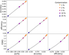
Fig. 1 Traditional deterministic metrics as a function of each other for increasing values (arrows) of the contamination parameter (c = 0.01, 0.02, 0.05, 0.10, 0.25), indicated in light orange, dark orange, pink, violet, and navy, respectively. Though these metrics are functions of the same four variables (see Equations (1), (2), (3), and (4)) and should thus be expected to have consistent relationships at all values of c, the detailed shapes depend on the values of the true and false positive and negative rates; this demonstrative plot thus reflects the proportions of SNe Ia and non-SNe Ia under the DDF observing strategy from Table 1 and our cosmological sample size of 𝒩 = 3000 (see Section 2.2.2). As anticipated, these metrics are degenerate with one another and are insensitive to the contaminating class makeup, only probing the contamination rate.
The summary statistics of estimated cosmological parameters: wfit assumes a Gaussian likelihood centered on the ΛCDM model and produces an estimated mean,
![Mathematical equation: $\[\hat{\mu}\]$](/articles/aa/full_html/2025/02/aa46891-23/aa46891-23-eq9.png) wfit, and standard deviation,
wfit, and standard deviation, ![Mathematical equation: $\[\hat{\sigma}\]$](/articles/aa/full_html/2025/02/aa46891-23/aa46891-23-eq10.png) wfit, whereas StanIa, on the other hand, yields posterior samples of w, which define a univariate probability density function (PDF). For the sake of comparison, we fit a normal distribution to the StanIa posterior samples of w to obtain
wfit, whereas StanIa, on the other hand, yields posterior samples of w, which define a univariate probability density function (PDF). For the sake of comparison, we fit a normal distribution to the StanIa posterior samples of w to obtain ![Mathematical equation: $\[\hat{\mu}\]$](/articles/aa/full_html/2025/02/aa46891-23/aa46891-23-eq11.png) StanIa and
StanIa and ![Mathematical equation: $\[\hat{\sigma}\]$](/articles/aa/full_html/2025/02/aa46891-23/aa46891-23-eq12.png) StanIa and observed their relative responses under different contamination levels and contaminant classes.
StanIa and observed their relative responses under different contamination levels and contaminant classes.-
Metrics of cosmology posterior PDFs: The posterior samples of w from the StanIa fit define a PDF, which we flexibly fit and evaluate on a fine grid using kernel density estimation (KDE), that is, eliminating the Gaussian assumption of the aforementioned cosmology metrics. We then performed a quantitative comparison of the KDEs
![Mathematical equation: $\[\hat{p}_{mock}(w)\]$](/articles/aa/full_html/2025/02/aa46891-23/aa46891-23-eq13.png) for each synthetic light curve sample by comparing them to that of the ‘perfect’ sample
for each synthetic light curve sample by comparing them to that of the ‘perfect’ sample ![Mathematical equation: $\[\hat{p}_{0}(w)\]$](/articles/aa/full_html/2025/02/aa46891-23/aa46891-23-eq14.png) by evaluating two metrics:
by evaluating two metrics:
-
The Kullback–Leibler divergence (KLD),
![Mathematical equation: $\[K L D=-\int \hat{p}_{0}(w) ~\ln~ \left[\frac{\hat{p}_{mock}(w)}{\hat{p}_{0}(w)}\right] d w,\]$](/articles/aa/full_html/2025/02/aa46891-23/aa46891-23-eq15.png) (5)
(5)is an information theoretic measure of the loss of information due to using an approximation,
![Mathematical equation: $\[\hat{p}_{mock}(w)\]$](/articles/aa/full_html/2025/02/aa46891-23/aa46891-23-eq16.png) , rather than the true distribution
, rather than the true distribution ![Mathematical equation: $\[\hat{p}_{0}(w)\]$](/articles/aa/full_html/2025/02/aa46891-23/aa46891-23-eq17.png) ; the KLD has been used before in extragalactic astrophysics (Malz et al. 2018; Kalmbach et al. 2020).
; the KLD has been used before in extragalactic astrophysics (Malz et al. 2018; Kalmbach et al. 2020). -
The Earth-Mover’s distance (EMD),
![Mathematical equation: $\[E M D=\int_{-\infty}^{\infty}\left|\int_{-\infty}^{w} \hat{p}_{0}(w^{\prime}) d w^{\prime}-\int_{-\infty}^{w} \hat{p}_{mock}(w^{\prime}) d w^{\prime}\right| d w,\]$](/articles/aa/full_html/2025/02/aa46891-23/aa46891-23-eq18.png) (6)
(6)also known as the first-order Wasserstein metric, can be intuitively understood as the integrated discrepancy between a pair of PDFs, defined in terms of their cumulative distribution functions (CDFs); the EMD has been used before in cosmology (e.g. Moews et al. 2021).
For both the KLD and EMD, lower values indicate a closer correspondence between distributions.
-
4 Analysis and results
Recalling that the goal of this investigation is to assess the degree to which classification metrics are consistent with metrics of cosmological constraints in the context of RESSPECT’s need for an internal metric to optimise classifications that are ultimately destined for SN Ia cosmology, we present a comprehensive comparison of various metrics evaluated on incrementally contaminated samples.
Our first goal is to quantify the effect on parameter inference due to sample size. Figure 2 shows posterior samples of w for the ‘perfect’, ‘random’, and ‘fiducial’ cases on mock cosmological light curve samples for different sample sizes. As the observed sensitivity of the posterior PDFs on w to sample size matches intuitive predictions (i.e. narrower for larger sample size), it is thus safe to use T P + F P = 3000 ‘post-classification’ light curves in our cosmological samples. The relatively small difference between the posterior widths for the DDF and WFD light curves could be considered a natural consequence of the fact that the samples include only light curves that survived a SALT2 fit and thus have error bars of comparable size on the distance moduli that enter the cosmology fits.
The tremendous gap between ‘random’ and the other two samples in the DDF is a direct consequence of the intrinsically higher S/N and sampling rate defining the DDF observing strategy. We also see that under DDF conditions, the constraints of the realistic ‘fiducial’ sample are close to the results for the ‘perfect’ sample. For the WFD, however, the distinction between the three cases is less pronounced, although the ‘random’ sample still outputs the largest biases independent of the sample size.
Figures 3 and 4 depict the behavior of our metrics as a function of the contaminant class and contamination level for the DDF and WFD observing strategies, respectively. Under both observing strategies, we note that the metrics of derived cosmological constraints are sensitive to both the contaminant class and the contamination rate, whereas the classification metric probes only the rate.
Under the DDF, in Figure 3, we observe that ΔF M shows a comparable impact for 2% SN II and 1% SN Ibc, and, separately for 5% SN II and 2% SN Ibc contamination, which are themselves on par with that of the random classification scheme, indicating that SN Ibc contaminants are effectively twice as damaging as SN II contaminants, and that random contamination isn’t much worse than that. However, the metrics derived from a full cosmological analysis tell a different story; the constraints from wfit and StanIa agree that even 1% contamination in the DDF with SN II skews the mean ![Mathematical equation: $\[\hat{w}\]$](/articles/aa/full_html/2025/02/aa46891-23/aa46891-23-eq19.png) beyond the 1-σ error bars of the pure sample, whereas even 5% SN Ibc or SN Iax do not. Critically, the bias due to even a low DDF contamination rate by SN II is on par with what would result from the realistic ‘fiducial’ classifier, a concern mirrored in the response of the metrics of the posterior PDFs of w from StanIa.
beyond the 1-σ error bars of the pure sample, whereas even 5% SN Ibc or SN Iax do not. Critically, the bias due to even a low DDF contamination rate by SN II is on par with what would result from the realistic ‘fiducial’ classifier, a concern mirrored in the response of the metrics of the posterior PDFs of w from StanIa.
For visualisation purposes, Figure 4 displays error bars corresponding to the greatest deviation from the mean across the ten trials rather than the standard deviation, except for the FOM3 metric, which lacks error bars because it is the same across all trials by construction. The most striking effect in Figure 4 is that the variation in metric values due to the random sample of included WFD light curves dominates over the impact of the different contaminant identities; there is a large range of light curve quality under the WFD observing strategy, and our relaxed sample selection criteria permit what amounts to only a few light curves to sway the cosmological constraints. Beyond that, we observe that 1% and 2% contamination by all classes are indistinguishable under the WFD by all cosmology metrics and do not induce a bias inconsistent with a pure sample nor the ‘fiducial’ mock classifier, a reassuring discovery. Though there is a weakly class-dependent effect at higher contamination rates according to the estimated mean and standard deviation on w by both fitting methods, which shows that 5% contamination with SN Iax is worse than 5% contamination by SN Ibc or SN II, the effect only persists at 10% contamination for wfit and at 25% for StanIa, suggesting a need for more WFD trials.
Figure 5 directly compares the relative response of the FOM3 classification metric and the KLD and EMD of posterior samples of the cosmological parameters for subsamples of varying contamination rate and contaminant within the DDF and WFD observing strategies. The clustering of points at discrete values of FOM3 are a result of its insensitivity to contaminant class, and the differentiation within each group demonstrates the sensitivity of the resulting cosmological parameter constraints to the type of contaminant at the same contamination rate. As is observed in Figures 3 and 4, we see stratification of cosmology metric values by contaminant class, somewhat suppressed in the WFD. This visualisation more directly highlights the conclusions from Figures 3 and 4, namely: (1) at a constant contamination rate, there are systematic, quantifiable differences in the derived cosmology depending on the contaminant class; (2) the effect establishes that contamination by SN II more strongly impacts the derived cosmology; (3) the variation between contaminant class is subdominant to the quality of the light curves under each observing strategy; (4) and both metrics of posterior samples of w are in qualitative agreement.
Figure 6 shows that the severity of bias in the estimated cosmological parameters as a function of the contaminant class is also related to how far off the estimated distance moduli are from the truth when fitting non-SN Ia with the SN Ia standardisation model, as expected. More importantly, it shows that individual contaminating light curves cannot, in general, be isolated from the SN Ia sample based on their fitted absolute magnitude, particularly at higher redshifts and under the WFD observing strategy. In effect, our mock sample generation procedure probes the most extreme bias that could be caused by each contaminant class. This test effectively includes redshift-dependent misclassification, which would lead to more of the brightest contaminants at higher redshift and those most similar to SN Ia in lower red-shifts, thus imposing a more subtle bias in the cosmological parameter constraints that would nonetheless not be reflected in the classification metrics alone.
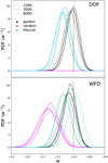 |
Fig. 2 StanIa posterior PDFs of w for different cosmological sample sizes (line styles) from the DDF and WFD observing strategies (panels) under the ‘perfect’ (black), ‘random’ (magenta), and ‘fiducial’ (cyan) mock classification schemes, with the true value of w indicated by a brown vertical line. We note that the ‘random’ classifier’s constraints in the DDF underestimate w by so much that they cannot be shown on these axes. As the constraints are not very sensitive to the sample size, we can safely use a cosmological sample of 3000 light curves in our tests. |
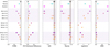 |
Fig. 3 Metrics summary for the DDF, with metric values on the x-axes and light curve samples on the y-axis, grouped by contaminant (shape and light purple backgrounds) and ranked by contamination fraction (color) aside from the ‘perfect’, ‘fiducial’, and ‘random’ light curve samples defined in Section 2.2, using the same colors for the named mock samples as in Figure 2. Reference values (vertical lines; dash-dotted black for the pure sample with 1-σ error regions in gray and solid brown for the truth) are provided where appropriate. The constraints on w (central two panels) include both the mean, |
![Mathematical equation: $\[\hat{w}\]$](/articles/aa/full_html/2025/02/aa46891-23/aa46891-23-eq20.png)
![Mathematical equation: $\[\sigma_{w}^{2}\]$](/articles/aa/full_html/2025/02/aa46891-23/aa46891-23-eq21.png)
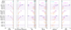 |
Fig. 4 Equivalent of Figure 3 for the WFD based on ten realisations of each sample. The plotted uncertainties in the constraints on w (central two panels) correspond to the largest |
![Mathematical equation: $\[\sigma_{w}^{2}\]$](/articles/aa/full_html/2025/02/aa46891-23/aa46891-23-eq22.png)
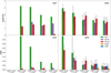 |
Fig. 5 The log-KLD and EMD of posterior samples of w at different values of the FOM3 classification metric for each contaminating class (color) and observing strategy (panel). The vertical lines within the WFD panels indicate the minimum and maximum values among ten different realizations. Despite the considerable variability between realizations, the cosmology metrics do exhibit consistent sensitivity to the impact of different classes of contaminant at a given contamination level. Examples of this effect manifest as stratification among the classes at a given FOM3 value. |
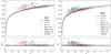 |
Fig. 6 Hubble diagram (upper) and residuals (lower) showing the ΛCDM model (solid black line) and two others depicting extreme dark energy behaviors (w = −2 - dashed, and w = 0 − dot-dashed). The gray points correspond to 2970 randomly selected SNe Ia from the available sample plus the low-z anchor SNe Ia, and the contaminants are shown at 1% contamination (class-specific shapes and colors) in DDF (left) and WFD (right). While some individual contaminant light curves have SALT2mu fit parameters far from those of the true SNe Ia, there is nontrivial overlap that would preclude simply classifying by eye to remove them from a sample entirely as expected given the selection criterion of a convergent SALT2mu fit); in the DDF, this effect is noticeable among the SN-Iax contaminants as well as SN-Ibc and SN-II at z > 0.8, whereas in the WFD, the problem is more severe, affecting all contaminants except CART and at redshifts as low as z > 0.2. |
5 Conclusions
Metrics of SNe Ia classification often serve as proxies for metrics of cosmological constraints derived from samples of light curves classified as SNe Ia, particularly in applications assessing the performance of light curve classifiers intended for cosmological analyses. In this work, we test the strength of the assumption underlying this usage and find that classification metrics are not always an appropriate substitute for metrics of cosmological parameters; the metrics of cosmological constraining power are sensitive to the composition of the contaminating populations as well as the contamination rate, but only the latter is probed by classification metrics. We thus recommend the use of cosmology-based metrics in place of classification metrics when optimising analysis pipeline designs, despite their associated computational expense (except when the light curves are noise-dominated).
In the context of RESSPECT, the above results confirm that relevant information is encapsulated in a metric of impact on cosmological constraints and must thus be considered as a factor in selecting spectroscopic follow-up candidates for inclusion in the training set within the active learning pipeline. More generically, as astronomical classifications are of course used for many other population-level studies, including and beyond transients, we encourage a healthy skepticism to those aiming to use such classifications in further scientific analyses. It would be prudent to confirm any correspondence between classification performance and metrics tailored to a specific science case prior to any decision-making on analysis approaches.
Acknowledgements
This paper has undergone internal review in the LSST Dark Energy Science Collaboration. The authors would like to thank Renée Hložek, Alex Kim, and Maria Vincenzi for serving as the LSST-DESC publication review committee, as well as David O. Jones, for his comments and suggestions that improved the quality of this manuscript. AIM acknowledges support during this work from the Max Planck Society and the Alexander von Humboldt Foundation in the framework of the Max Planck-Humboldt Research Award endowed by the Federal Ministry of Education and Research. A.I.M. is supported by Schmidt Sciences. M.D. is supported by the Horizon Fellowship at the Johns Hopkins University. S.G.G. acknowledges support by FCT under Project CRISP PTDC/FIS-AST-31546/2017 and UIDB/00099/2020. L.G. acknowledges financial support from the Spanish Ministry of Science and Innovation (MCIN) under the 2019 Ramon y Cajal program RYC2019-027683 and from the Spanish MCIN project HOSTFLOWS PID2020-115253GA-I00. This work is financially supported by CNRS as part of its MOMENTUM programme under the project Adaptive Learning for Large Scale Sky Surveys. The Cosmostatistics Initiative (COIN, https://cosmostatistics-initiative.org/) is an international network of researchers whose goal is to foster interdisciplinarity inspired by Astronomy. The DESC acknowledges ongoing support from the Institut National de Physique Nucléaire et de Physique des Particules in France; the Science & Technology Facilities Council in the United Kingdom; and the Department of Energy, the National Science Foundation, and the LSST Corporation in the United States. DESC uses resources of the IN2P3 Computing Center (CC-IN2P3–Lyon/Villeurbanne – France) funded by the Centre National de la Recherche Scientifique; the National Energy Research Scientific Computing Center, a DOE Office of Science User Facility supported by the Office of Science of the U.S. Department of Energy under Contract No. DE-AC02-05CH11231; STFC DiRAC HPC Facilities, funded by UK BIS National E-infrastructure capital grants; and the UK particle physics grid, supported by the GridPP Collaboration. This work was performed in part under DOE Contract DE-AC02-76SF00515. Author contributions. A.I. Malz: conceptualisation, formal analysis, investigation, methodology, software, validation, visualisation, writing – original draft, writing – review & editing; M. Dai: data curation, formal analysis, investigation, methodology, software, validation, writing – review & editing; K.A. Ponder: conceptualisation, formal analysis, investigation, methodology, software, validation, visualization, writing – original draft; E.E.O. Ishida: conceptualisation, data curation, formal analysis, funding acquisition, project administration, resources, software, supervision, validation, visualisation, writing – original draft, writing – review & editing; S. Gonzalez-Gaitain: conceptualisation, methodology, software, writing – review & editing; R. Durgesh: software; A. Krone-Martins: funding acquisition, project administration, resources, software, supervision; R.S. de Souza: funding acquisition, project administration, resources, supervision; N. Kennamer: software, methodology; S. Sreejith: software; L. Galbany: conceptualisation.
References
- Albrecht, A., Bernstein, G., Cahn, R., et al. 2006, arXiv e-prints [arXiv:astro-ph/0609591] [Google Scholar]
- Astier, P., Guy, J., Regnault, N., et al. 2006, A&A, 447, 31 [NASA ADS] [CrossRef] [EDP Sciences] [Google Scholar]
- Bellm, E. C., Kulkarni, S. R., Graham, M. J., et al. 2019, PASP, 131, 018002 [Google Scholar]
- Betoule, M., Kessler, R., Guy, J., et al. 2014, A&A, 568, A22 [NASA ADS] [CrossRef] [EDP Sciences] [Google Scholar]
- Boone, K. 2019, AJ, 158, 257 [NASA ADS] [CrossRef] [Google Scholar]
- Carrick, J. E., Hook, I. M., Swann, E., et al. 2021, MNRAS, 508, 1 [Google Scholar]
- Dark Energy Survey Collaboration (Abbott, T., et al.) 2016, MNRAS, 460, 1270 [Google Scholar]
- DES Collaboration (Abbott, T. M. C., et al.) 2018, arXiv e-prints [arXiv:1811.02374] [Google Scholar]
- Gris, P., Regnault, N., Awan, H., et al. 2023, ApJS, 264, 22 [NASA ADS] [CrossRef] [Google Scholar]
- Guy, J., Astier, P., Baumont, S., et al. 2007, A&A, 466, 11 [NASA ADS] [CrossRef] [EDP Sciences] [Google Scholar]
- Hinton, S., & Brout, D. 2020, J. Open Source Softw., 5, 2122 [NASA ADS] [CrossRef] [Google Scholar]
- Hlozek, R., Kunz, M., Bassett, B., et al. 2012, ApJ, 752, 79 [NASA ADS] [CrossRef] [Google Scholar]
- Hložek, R., Malz, A. I., Ponder, K. A., et al. 2023, ApJS, 267, 25 [Google Scholar]
- Holtzman, J. A., Marriner, J., Kessler, R., et al. 2008, AJ, 136, 2306 [NASA ADS] [CrossRef] [Google Scholar]
- Hounsell, R., Scolnic, D., Foley, R. J., et al. 2018, ApJ, 867, 23 [NASA ADS] [CrossRef] [Google Scholar]
- Ishida, E. E. O. 2019, Nat. Astron., 3, 680 [NASA ADS] [CrossRef] [Google Scholar]
- Ishida, E. E. O., Beck, R., González-Gaitán, S., et al. 2019, MNRAS, 483, 2 [Google Scholar]
- Jones, D. O., Scolnic, D. M., Riess, A. G., et al. 2018, ApJ, 857, 51 [NASA ADS] [CrossRef] [Google Scholar]
- Jones, D. O., Scolnic, D. M., Foley, R. J., et al. 2019, ApJ, 881, 19 [Google Scholar]
- Kalmbach, J. B., VanderPlas, J. T., & Connolly, A. J. 2020, ApJ, 890, 74 [NASA ADS] [CrossRef] [Google Scholar]
- Kennamer, N., Ishida, E. E. O., González-Gaitán, S., et al. 2020, in 2020 IEEE Symposium Series on Computational Intelligence (SSCI), 3115 [CrossRef] [Google Scholar]
- Kessler, R., & Scolnic, D. 2017, ApJ, 836, 56 [Google Scholar]
- Kessler, R., Bernstein, J. P., Cinabro, D., et al. 2009, PASP, 121, 1028 [Google Scholar]
- Kessler, R., Bassett, B., Belov, P., et al. 2010, PASP, 122, 1415 [CrossRef] [Google Scholar]
- Kessler, R., Narayan, G., Avelino, A., et al. 2019, PASP, 131, 094501 [NASA ADS] [CrossRef] [Google Scholar]
- LSST Science Collaboration (Abell, P. A., et al.) 2009, arXiv e-prints [arXiv:0912.0201] [Google Scholar]
- Malz, A. I., Marshall, P. J., DeRose, J., et al. 2018, AJ, 156, 35 [CrossRef] [Google Scholar]
- Malz, A. I., Hložek, R., Allam, T., J., et al. 2019, AJ, 158, 171 [NASA ADS] [CrossRef] [Google Scholar]
- Marriner, J., Bernstein, J. P., Kessler, R., et al. 2011, ApJ, 740, 72 [NASA ADS] [CrossRef] [Google Scholar]
- Moews, B., Schmitz, M. A., Lawler, A. J., et al. 2021, MNRAS, 500, 859 [Google Scholar]
- Möller, A., & de Boissière, T. 2020, MNRAS, 491, 4277 [CrossRef] [Google Scholar]
- Muthukrishna, D., Narayan, G., Mandel, K. S., Biswas, R., & Hložek, R. 2019, PASP, 131, 118002 [NASA ADS] [CrossRef] [Google Scholar]
- Pasquet, J., Pasquet, J., Chaumont, M., & Fouchez, D. 2019, A&A, 627, A21 [NASA ADS] [CrossRef] [EDP Sciences] [Google Scholar]
- Perlmutter, S., Aldering, G., Goldhaber, G., et al. 1999, ApJ, 517, 565 [Google Scholar]
- PLAsTiCC-Modelers 2019, https://doi.org/10.5281/zenodo.2612896 [Google Scholar]
- Popovic, B., Scolnic, D., & Kessler, R. 2020, ApJ, 890, 172 [NASA ADS] [CrossRef] [Google Scholar]
- Rest, A., Scolnic, D., Foley, R. J., et al. 2014, ApJ, 795, 44 [Google Scholar]
- Riess, A. G., Filippenko, A. V., Challis, P., et al. 1998, AJ, 116, 1009 [Google Scholar]
- Rose, B. M., Baltay, C., Hounsell, R., et al. 2021, arXiv e-prints [arXiv:2111.03081] [Google Scholar]
- The PLAsTiCC team, Allam, T. Jr., Bahmanyar, A., et al. 2018, arXiv e-prints [arXiv:1810.00001] [Google Scholar]
- The LSST Dark Energy Science Collaboration, Mandelbaum, R., Eifler, T., et al. 2018, arXiv e-prints [arXiv:1809.01669] [Google Scholar]
- Villar, V. A., Hosseinzadeh, G., Berger, E., et al. 2020, ApJ, 905, 94 [NASA ADS] [CrossRef] [Google Scholar]
- Vincenzi, M., Sullivan, M., Möller, A., et al. 2022, MNRAS, 518, 1106 [NASA ADS] [CrossRef] [Google Scholar]
- Wood-Vasey, W. M., Miknaitis, G., Stubbs, C. W., et al. 2007, ApJ, 666, 694 [NASA ADS] [CrossRef] [Google Scholar]
The effect caused by false negatives is outside the scope of this work.
Only 32% of the objects in the original data survived this procedure.
See SNANA manual, Section 11 at https://github.com/RickKessler/SNANA/blob/master/doc/snana_manual.pdf
All Tables
The populations of light curves under each survey strategy that survive a SALT2 fit, as well as the survivor fraction after the SALT2 fit criterion.
All Figures
|
Fig. 1 Traditional deterministic metrics as a function of each other for increasing values (arrows) of the contamination parameter (c = 0.01, 0.02, 0.05, 0.10, 0.25), indicated in light orange, dark orange, pink, violet, and navy, respectively. Though these metrics are functions of the same four variables (see Equations (1), (2), (3), and (4)) and should thus be expected to have consistent relationships at all values of c, the detailed shapes depend on the values of the true and false positive and negative rates; this demonstrative plot thus reflects the proportions of SNe Ia and non-SNe Ia under the DDF observing strategy from Table 1 and our cosmological sample size of 𝒩 = 3000 (see Section 2.2.2). As anticipated, these metrics are degenerate with one another and are insensitive to the contaminating class makeup, only probing the contamination rate. |
| In the text | |
|
Fig. 2 StanIa posterior PDFs of w for different cosmological sample sizes (line styles) from the DDF and WFD observing strategies (panels) under the ‘perfect’ (black), ‘random’ (magenta), and ‘fiducial’ (cyan) mock classification schemes, with the true value of w indicated by a brown vertical line. We note that the ‘random’ classifier’s constraints in the DDF underestimate w by so much that they cannot be shown on these axes. As the constraints are not very sensitive to the sample size, we can safely use a cosmological sample of 3000 light curves in our tests. |
| In the text | |
|
Fig. 3 Metrics summary for the DDF, with metric values on the x-axes and light curve samples on the y-axis, grouped by contaminant (shape and light purple backgrounds) and ranked by contamination fraction (color) aside from the ‘perfect’, ‘fiducial’, and ‘random’ light curve samples defined in Section 2.2, using the same colors for the named mock samples as in Figure 2. Reference values (vertical lines; dash-dotted black for the pure sample with 1-σ error regions in gray and solid brown for the truth) are provided where appropriate. The constraints on w (central two panels) include both the mean, |
| In the text | |
|
Fig. 4 Equivalent of Figure 3 for the WFD based on ten realisations of each sample. The plotted uncertainties in the constraints on w (central two panels) correspond to the largest |
| In the text | |
|
Fig. 5 The log-KLD and EMD of posterior samples of w at different values of the FOM3 classification metric for each contaminating class (color) and observing strategy (panel). The vertical lines within the WFD panels indicate the minimum and maximum values among ten different realizations. Despite the considerable variability between realizations, the cosmology metrics do exhibit consistent sensitivity to the impact of different classes of contaminant at a given contamination level. Examples of this effect manifest as stratification among the classes at a given FOM3 value. |
| In the text | |
|
Fig. 6 Hubble diagram (upper) and residuals (lower) showing the ΛCDM model (solid black line) and two others depicting extreme dark energy behaviors (w = −2 - dashed, and w = 0 − dot-dashed). The gray points correspond to 2970 randomly selected SNe Ia from the available sample plus the low-z anchor SNe Ia, and the contaminants are shown at 1% contamination (class-specific shapes and colors) in DDF (left) and WFD (right). While some individual contaminant light curves have SALT2mu fit parameters far from those of the true SNe Ia, there is nontrivial overlap that would preclude simply classifying by eye to remove them from a sample entirely as expected given the selection criterion of a convergent SALT2mu fit); in the DDF, this effect is noticeable among the SN-Iax contaminants as well as SN-Ibc and SN-II at z > 0.8, whereas in the WFD, the problem is more severe, affecting all contaminants except CART and at redshifts as low as z > 0.2. |
| In the text | |
Current usage metrics show cumulative count of Article Views (full-text article views including HTML views, PDF and ePub downloads, according to the available data) and Abstracts Views on Vision4Press platform.
Data correspond to usage on the plateform after 2015. The current usage metrics is available 48-96 hours after online publication and is updated daily on week days.
Initial download of the metrics may take a while.