| Issue |
A&A
Volume 693, January 2025
|
|
|---|---|---|
| Article Number | A186 | |
| Number of page(s) | 9 | |
| Section | The Sun and the Heliosphere | |
| DOI | https://doi.org/10.1051/0004-6361/202452938 | |
| Published online | 15 January 2025 | |
Non-local thermal transport impact on compressive waves in two-temperature coronal loops
1
Centre for Fusion, Space and Astrophysics, Department of Physics, University of Warwick, Coventry CV4 7AL, UK
2
Healthcare Technology Institute, School of Chemical Engineering, The University of Birmingham, Birmingham, UK
3
Engineering Research Institute “Ventspils International Radio Astronomy Centre (VIRAC)”, Ventspils University of Applied Sciences, Ventspils LV-3601, Latvia
⋆ Corresponding author; This email address is being protected from spambots. You need JavaScript enabled to view it.
Received:
8
November
2024
Accepted:
7
December
2024
Abstract
Context. Observations of slow magnetoacoustic waves in solar coronal loops suggest that in hot coronal plasma, heat conduction may be suppressed in comparison with the classical thermal transport model.
Aims. We link this suppression with the effect of the non-local thermal transport that appears when the plasma temperature perturbation gradient becomes comparable to the electron mean-free-path. Moreover, we consider a finite time of thermalisation between electrons and ions so that separate electron and ion temperatures can occur in the loop.
Methods. We numerically compared the influence of the local and non-local thermal transport models on standing slow waves in one- and two-temperature coronal loops. To quantify our comparison, we used the period and damping time of the waves as commonly observed parameters.
Results. Our study reveals that non-local thermal transport can result in either shorter or longer slow-wave damping times in comparison with the local conduction model due to the suppression of the isothermal regime. The difference in damping times can reach 80%. For hot coronal loops, we find that the finite equilibration between electron and ion temperatures results in an up to 50% longer damping time compared to the one-temperature case. These results indicate that non-local transport will influence the dynamics of compressive waves across a broad range of coronal plasma parameters with Knudsen numbers (the ratio of mean-free-path to temperature scale length) larger than 1%.
Conclusions. In the solar corona, the non-local thermal transport shows a significant influence on the dynamics of standing slow waves in a broad range of plasma parameters, while two-temperature effects come into play for hot and less dense loops.
Key words: conduction / waves / Sun: corona / Sun: oscillations
© The Authors 2025
 Open Access article, published by EDP Sciences, under the terms of the Creative Commons Attribution License (https://creativecommons.org/licenses/by/4.0), which permits unrestricted use, distribution, and reproduction in any medium, provided the original work is properly cited.
This article is published in open access under the Subscribe to Open model. This email address is being protected from spambots. You need JavaScript enabled to view it. to support open access publication.
1. Introduction
Standing slow waves in the solar corona were first observed as periodic variations of the Doppler shift in hot lines (Wang et al. 2002, 2003; Mariska 2005, 2006). Named after the Solar Ultraviolet Measurement of Emitted Radiation (SUMER) spectrometer on board the Solar and Heliospheric Observatory, these oscillations are called SUMER oscillations. Later, standing slow waves associated with SUMER oscillations in flaring coronal loops were detected by imaging observations (Wang et al. 2015; Nisticò et al. 2017). The intrinsic feature of SUMER oscillations is a rapid decay with characteristic times comparable to their periods. These damping times can be used as seismological information to determine the transport coefficients in coronal plasma (Wang et al. 2018; Wang & Ofman 2019) and constrain the coronal heating function (Reale et al. 2019; Kolotkov et al. 2020).
At the same time, there is evidence of standing slow waves existing in cooler coronal loops obtained by spectroscopic and imaging instruments. Using the extreme UV imaging-spectrometer Hinode/EIS, Erdélyi & Taroyan (2008) analysed oscillations of intensity and Doppler shift along coronal loop-like structures with 1–2 MK temperatures. Due to the quarter-period phase shift between the intensity and the Doppler shift, these oscillations were explained as standing slow waves. Using the same instrument for Fe XII, Fe XIII, Fe XIV, and Fe XV coronal lines, Mariska et al. (2008) observed the Doppler shift oscillations with the amplitude of about 2 km/s and a period of around 35 minutes, which is consistent with the explanation in terms of standing slow waves. For these observations, the damping time increased with increasing temperature. For the Fe XII line (the lowest formation temperature), the damping time was 42 minutes, while for the Fe XV line (the highest formation temperature), no damping was observed. For the latter, the lack of slow-wave damping was attributed to the effect of thermal misbalance in Kolotkov et al. (2019). For coronal fan loops, Pant et al. (2017) reported imaging observations of standing slow waves with a period and damping time of about 25 and 45 minutes, respectively.
Statistical analysis made by Nakariakov et al. (2019) shows that there is a gap in observations of standing slow waves between hot coronal loops with temperatures of 6–14 MK, where these waves are predominantly observed, and cold and warm coronal loops with temperatures of 0.6–2 MK. For hot coronal loops, one may expect the field-aligned thermal conduction to be the main actor for the slow wave dynamics. However, the seismologic measurement of the polytropic index using a standing slow wave in a 10 MK loop showed a value near 1.64 (Wang et al. 2015). Since this value is close to the adiabatic index 5/3 for an ideal monatomic gas, Wang et al. (2015) suggested that the thermal conduction should be suppressed in the hot flare loops by at least a factor of three. For 1.7 MK plasma, Van Doorsselaere et al. (2011) estimated the polytropic index to be 1.10 using slow waves propagating upward from active region footpoints. The measured value is close to the isothermal adiabatic index of one, which suggests that thermal conduction is important in these conditions. Moreover, unlike (Wang et al. 2015), the thermal conduction value inferred from the measured phase shift was comparable to the classical value (Spitzer & Härm 1953). On the other hand, when investigating propagating slow waves in fan loops, Prasad et al. (2018) found that the polytropic index varied from 1.04 to 1.58, being higher for hotter loops, while the temperature range considered was approximately 0.9–1.1 MK. It should be mentioned that all of these inferences on the role of conduction were made in the polytropic assumption. It was shown by Kolotkov (2022) that this assumption can be used in the corona only in a weakly conductive regime when the effective polytropic index weakly deviates from its adiabatic value of 5/3.
When fitting polytropic models with conduction to the damping of slow waves, the higher values of the polytropic index inferred for hotter loops are in contradiction to the classical thermal conduction theory (Spitzer & Härm 1953), which would predict a decrease in the inferred polytropic index with temperature (see e.g. Fig. 5 from Kolotkov 2022). The heat fluxes predicted by this local thermal transport model depend on the local temperature gradient. It assumes that the thermal electron mean-free path is much less than the characteristic length scales of the temperature gradient. However, as the temperature increases, the mean-free path can become comparable with the characteristic length scales, and hot electrons from the tail of the electron distribution can travel for longer distances between effective collisional scattering. This makes the local thermal transport model invalid and demands using a non-local model based on solving the Vlasov-Fokker-Planck equation (Arber et al. 2023). The main effects described by the non-local models of thermal transport are the broadening of the heat flux effective spatial profile (also referred to as pre-heating, and it is caused by hotter electrons carrying energy for longer distances) and an overall suppression of heat fluxes. In other words, non-local thermal transport models allow for mitigating the infinite increase of the heat flux with temperature in the classical thermal conduction theory by Spitzer & Härm (1953). In the case of coronal loops, this suppression may result in an increase in coronal cooling times (West et al. 2004, 2008). This suggests that non-local thermal transport may explain the suppression of thermal conduction observed by using slow waves (Wang et al. 2015; Prasad et al. 2018) and in solar flare observations (Battaglia et al. 2009; Fleishman et al. 2023). However, the influence of the non-local thermal effects on slow waves has yet to be studied.
In this work, we compare the influence of the local and non-local thermal transport models on standing compressive waves for a broad range of coronal plasma conditions. Also, we examine how finite equilibration between ion and electron temperatures affect the wave dynamics. The paper is organised as follows. In Section 2, we describe the numerical code and the thermal transport models used in this study. In Section 3, we conduct a parametric study of the thermal transport influence on standing slow waves in one- and two-temperature coronal loops. Finally, we draw our conclusions in Section 4.
2. Numerical model
In this study, we use the Freyja code. It is a two-temperature hydrodynamics code designed originally for simulating laser plasma experiments (e.g. Paddock et al. 2023) and solves the equations for mass and momentum conservation coupled to non-adiabatic equations for the specific internal energies of the ion and electron species of a plasma:
 (1)
(1)
 (2)
(2)
 (3)
(3)
 (4)
(4)
Here, we used the hydrodynamical model without taking magnetic field perturbations into account because in the low-β plasma, slow waves result in perturbations of the magnetic field that are much smaller than the density and temperature perturbations (e.g. Ofman & Wang 2022). This 1D approach for modelling slow waves in the corona is also known as the infinite field approximation (see Wang et al. 2021, Sect. 2.3 and references therein).
The core hydrodynamics equations were solved in the Lagrangian frame using a compatible energy update (Caramana et al. 1998a). The term QVisc represents a shock viscosity (Caramana et al. 1998b). The viscous heating only impacts the ion equation, and PT = Pi + Pe represents the total hydrodynamical pressure. The specific internal energies ϵi, e are the internal energies of the ions and electrons divided by the total (electron and ion) mass density. The plasma was assumed to be fully ionised hydrogen, with an ideal gas equation of state,
 (5)
(5)
where γ = 5/3.
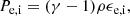
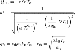
The term Sequil represents the change in temperature due to collisional temperature equilibration of the ion and electron species. The rate of change of the electron temperature is given by
 (6)
(6)
where the equilibration time τei is given by the inverse of the collision frequency:
 (7)
(7)
where me, i, ne, i, Te, i, Ze, i are masses, number densities, temperatures, and charge numbers of electrons and ions, respectively; kB is the Boltzmann constant; and λei is the electron-ion Coulomb logarithm. To justify the importance of treating electron and ion temperatures separately in our study, we have plotted the equilibration time τei in the left panel of Fig. 1 for a wide set of coronal densities and temperatures. This plot shows that this time may vary from a fraction of a second to several thousand seconds. The right panel of Fig. 1 compares this time with the period P of the fundamental standing slow mode in an adiabatic plasma calculated as P = 2L0/cs, where L0 = 100 Mm is the loop length and cs is the adiabatic sound speed. It can be seen that there is a region where τei is comparable with wave periods, and therefore, this effect should be taken into account in the study.
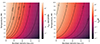 |
Fig. 1. Equilibration time τei importance under coronal conditions. Left panel: equilibration time τei contours as a function of the plasma number density and temperature. Right panel: relation between the equilibration time τei and a period P of a fundamental standing mode in a 100 Mm loop in adiabatic plasma as a function of the plasma number density and temperature. |
In this work, ion thermal conduction is neglected. The term SCond. in Eq. (4) represents the heat flux:
 (8)
(8)
The electron heat flux, q can be calculated either as a heat flux obtained for short mean-free-paths by using Spitzer-Härm (SH) approximation (Spitzer & Härm 1953) QSH, the flux-limited (FL) local heat flux QFL, or the non-local heat flux obtained with the Schurtz-Nicolaï-Busquet (SNB) model (Schurtz et al. 2000; Brodrick et al. 2017) QSNB. The SH heat flux is calculated as follows:
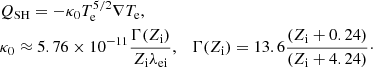 (9)
(9)
For fully ionised hydrogen plasma, Zi = 1, and λei = 18.5 is frequently assumed for the coronal conditions, giving κ0 ≈ 10−11. While this SH approximation is common in solar coronal studies, it is only a valid approximation for Knudsen numbers 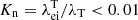 , where
  is the electron thermal mean-free path, and λT is the temperature gradient length scale.
In regions of steep temperature gradients, the predicted SH flux can become unphysical. For example, the total heat flux is unlikely to be larger than the total local thermal energy density advected at the thermal speed, the so-called free-streaming limit heat flux: qfs = vthnekBTe. As a result, the heat flux is often limited to make sure it is less than this limit. The FL local heat flux was calculated by applying a Larsen limiter (Olson et al. 2000) to the Spitzer-Härm flux:
 (10)
(10)
where α is the maximum fraction of the free-streaming flux permitted. Typically, this is between 0.01 and 0.2 and is usually determined by the best fit to observations. This limits the predictive power of this approach.
The heat flux in the SH model is primarily carried by electrons with speeds of ≃3 vth. Since the mean-free-path scales with speed to the fourth power, such electrons have mean-free-paths ≃100 times larger than the thermal mean-free-path. Hence, SH is expected to be inaccurate once Kn > 0.01. A full treatment of heat conduction in this regime requires a Vlasov-Focker-Planck (VFP) solution. This is too complex to be included in a fluid code, and instead a simplified model, the SNB model, is often used. The SNB model is an approximate solution of the full VFP equation divided into energy bins (for the derivation outline see Schurtz et al. 2000; Brodrick et al. 2017). These energy bins are introduced to approximate the distribution function. The simplified VFP equation is solved for each energy bin, and the solutions are combined to calculate a correction to the local SH heat flux QSH. The non-local heat flux obtained with the SNB model (Schurtz et al. 2000; Brodrick et al. 2017) is
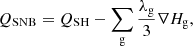 (11)
(11)
where the function Hg is calculated by solving ODE (15) from Arber et al. (2023) for each energy group Eg with λg2 = λeeλei, where λee and λei are electron-electron and electron-ion mean-free paths (for the details see Arber et al. 2023).
To illustrate the differences between the aforementioned thermal transport models, we calculated the heat fluxes for the initial Gaussian perturbation of plasma temperature in the form T = T0 + 0.01T0exp(−x2/σ2), where T0 = 1 MK, σ = 5 Mm, and the plasma number density is n0 = 109 cm−3 by using Eqs. (9), (10), and (11). The SNB heat flux was calculated by adopting the python script from Arber et al. (2023)1. The calculated heat fluxes are shown in the left panel of Fig. 2. It can be seen that SNB results in a suppression of the heat flux, and it spreads in a wider region compared to the local SH and FL models. This pre-heat is due to the high-energy tail of the electron distribution. Thus SH over-estimates the heat flux for Kn > 0.01. This reduction in heat flux can be approximated using the FL model but only once the answer is known so that α can be specified. The SNB model has no free parameters and predicts both the flux suppression and pre-heat.
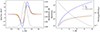 |
Fig. 2. Comparison between the SH, FL, and SNB thermal transport models. Left panel: initial Gaussian perturbation of temperature (black dotted curve) and heat fluxes corresponding to this perturbation for the case of the SH (blue solid curve), SNB (green dashed curve), and FL (red dashed curve) thermal transport models. The orange shading denotes the regions where pre-heating takes place (the effective width of the heat flux predicted by SNB is greater than that by SH and than the width of the initial temperature perturbation). Right panel: peak SH (blue solid curve), SNB (green dashed curve), and FL (red dashed curve) heat fluxes measured in units of maximum SH heat flux at 1 MK (Q0). The black dotted curve denotes the relation of maximum SNB heat flux over the corresponding maximum SH heat flux. |
With an increase in temperature, the maximum heat flux value increases for all models considered (see blue, green, and red curves in the right panel of Fig. 2). However, this growth is significantly slower for the FL and SNB models. Moreover, the results for the FL model are subject to the choice of the parameter α. For the SNB case, the effective reduction of heat flux in comparison to the SH model is connected with the increase in the electron mean-free-path with temperature. The black curve in the right panel of Fig. 2 demonstrates that QSNB decreases with increasing temperature from QSNB ≈ 0.7 QSH at T0 = 1 MK to QSNB ≈ 0.008 QSH at T0 = 10 MK.
3. Numerical simulations
3.1. Slow wave mode set up
To simulate standing slow waves, we used 1000 uniformly spaced grid points and reflecting boundary conditions assuring a zero thermal flux through the boundaries. The shock viscosity was switched off since all the simulations are linear and do not involve any shocks. To initialise the fundamental standing mode, we set up the initial velocity perturbation as
 (12)
(12)
where cs is a sound speed and L0 is a length of the loop that is equal to the size of the domain. All runs were performed for a set of loop parameters listed in Table 1 using the following thermal transport models: SH, FL, and SNB. For the SNB model, we used 50 energy bins uniformly spread between 0 and 20kBT0 to assure both adequate energy resolution and computational speed.
Set of the loop parameters used in the study.
Figure 3 shows examples of the velocity evolution at the loop apex for the considered models of thermal transport in the one-temperature (left panel) and two-temperature (right panel) regimes. It follows from the plot that the two-temperature regime results in slower damping of standing waves. Also, it can be seen that the difference between non-local and local thermal transport is not negligible. At the same time, the SNB and FL models almost coincide at T0 = 1 MK for the chosen value of the flux-limiting parameter α = 0.0001 and diverge with the increase in temperature. This demonstrates that the choice of the flux-limiting parameter α = 0.0001 is problem-dependent, and it is impossible to use the same value of α for all domains of the plasma considered. Moreover, at T0 = 10 MK, the FL model shows apparent non-exponential damping (the oscillation amplitude approaches a stationary level), while the damping is exponential in the SH and SNB cases. This non-exponential damping is attributed to the form of flux limiting and is therefore non-physical. For the reasons mentioned above, we focused on the comparison between the SH and SNB models.
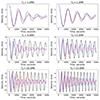 |
Fig. 3. Examples of velocity perturbations at the apex of a loop with L = 100 Mm and n0 = 108 cm−3 for SH (black solid curve), SNB (red dashed curve), and FL with α = 0.0001 (blue dashed curve) in the one-temperature (left column) and two-temperature (right column) regimes. |
3.2. One-temperature (magnetohydrodynamic) regime
To initially separate the effects of non-local thermal transport from the effect of the finite equilibration time τei, we multiplied the value of τei, calculated using Eq. (7), by 10−20, effectively making temperature equilibration instantaneous. This guarantees that plasma is in the magnetohydrodynamic (MHD), or one-temperature, regime. Next, to separate the local thermal transport regime from the non-local one, it is worth using Knudsen number  . Usually, the temperature length scale is determined as λT = T(dT/dx)−1; however, in this work, we used λT = L0 since we study small perturbations of uniform background and may underestimate λT. It was shown that the local thermal transport approximation fails for Kn > 0.01, and non-local effects take place (Arber et al. 2023). Figure 4 demonstrates the critical temperature gradient scale length
  ; when
  , the local thermal transport may be violated. For example,
  Mm for hot coronal plasma, which is comparable with the loop lengths observed.
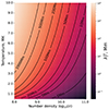 |
Fig. 4. Critical temperature length scale |


To check the difference between the local and non-local thermal transport models, we used the velocity profiles at the middle of the numerical domain (as in Fig. 3) and fit them with the decaying harmonic function v(x = 0.5L0,t) ∝ e−t/τsin(2πt/P+ϕ0) with initial phase ϕ0 to retrieve the oscillation period P and damping time τ as potential observables. A similar approach was used by Wang et al. (2015) to retrieve the parameters of slow-mode waves in a flaring loop. Thus, using these parameters, we could estimate how the different thermal transport models affect slow wave dynamics for the different coronal plasma conditions.
The left panel of Fig. 5 shows the relative difference between the damping time of slow waves with non-local thermal transport τSNB and the damping time for the local thermal transport model τSH together with Kn contours for the one-temperature regime for coronal loops with L0 = 100 Mm (cf. Fig. 6 for solar flares in Battaglia et al. 2009). As one can see from Fig. 5, the damping of slow waves with the SNB model can be more and less effective than with the SH model, and the absolute value of the difference between damping times can reach 80%. The border between the regimes of faster or slower damping is found to be near Kn = 0.01. Since non-local thermal transport results in thermal flux suppression, faster damping of slow waves seems to be a contradiction in this case. However, this faster damping can be explained by the left panel of Fig. 6 showing the dependencies of SNB and SH damping times on temperature for the plasma number density n0 = 109 cm−3. Validating the results of our numerical simulations, Fig. 6 also shows the dependence of the SH damping time on temperature, obtained from the dispersion relation of a slow-mode wave in one-temperature plasma with thermal conduction (see e.g. Eq. (19) in De Moortel & Hood 2003). Thus, for the SH case, the damping time curve reaches a minimum near 3 MK. Up to this value, an increasing temperature results in an increase in thermal conductivity and a consequent reduction in the damping time due to conduction. However, for very high temperatures, conduction is so rapid that the oscillations approach the isothermal limit. In this regime, conduction can have no effect on the damping of the slow mode, and thus the damping time increases. This explains the increase in damping time after the minimum (see also the left panel of Fig. 3). Thus, we can conclude that for the SH model, the waves gradually approach an isothermal regime after 3 MK. In the SNB case, in contrast, the heat-flux suppression due to non-local thermal transport results in the damping time minimum being shifted to higher temperatures (≳10 MK, according to Fig. 6). Therefore, SNB non-local conduction causes a delayed onset of the isothermal regime compared to SH.
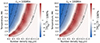 |
Fig. 5. Relative difference between SNB and SH damping times of slow waves for the one-temperature (left panel) and two-temperature (right panel) plasma regimes. The plot was obtained by using cubic interpolation of the results from a 0.5 × 0.5 grid cell to a 0.1 × 0.1 grid cell. |
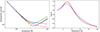 |
Fig. 6. Comparison of slow-wave damping times between the SH and SNB thermal transport models. Left panel: slow-wave damping times for SH in the one-temperature (orange solid curve) and two-temperature (green solid curve) regimes and SNB in the one-temperature (red dashed curve) and two-temperature (blue dashed curve) plasma with n0 = 109 cm−3. The black crosses represent the damping time calculated by solving a dispersion relation (see e.g. Eq. (19) in De Moortel & Hood 2003) for one-temperature plasma with the SH thermal transport model. Right panel: ratio of SNB and SH damping times for one-temperature (red solid curve) and two-temperature (blue dashed curve) plasma with n0 = 109 cm−3. |
The right panel of Fig. 6 shows how the ratio between SNB and SH damping times changes with temperature for plasma number density n0 = 109 cm−3. It can be seen that the deviation between SNB and SH damping times is non-monotonic, with the increase in temperature corresponding to a Kn increase. Initially, the SNB damping time grows in comparison with the SH case and drops down as soon as waves approach the isothermal regime in the SH case.
The left panel of Fig. 7 represents the relative difference of the measured periods of slow standing waves for the SNB (PSNB) and the SH (PSH) models for the one-temperature regime as it was shown for the damping time τ in Fig. 5. The region where the difference is noticeable starts from the Kn = 0.01 contour. The difference is negative inside this domain, and it means that the period of standing waves is shorter for the case of non-local thermal transport, and therefore, their phase speed is higher. For the local thermal transport case, the phase speed of slow waves decreases from the usual sound speed to the isothermal sound speed. As the non-local thermal transport prevents slow waves from switching to the isothermal regime, the phase speed of slow waves decreases more slowly than in the case of local thermal transport and, thus, yields a negative difference in periods. In this regard, non-local transport allows the periods of slow waves to remain closer to their values in the adiabatic plasma.
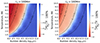 |
Fig. 7. Relative difference between SNB and SH periods of slow waves for the one-temperature (left panel) and two-temperature (right panel) plasma regimes. The plot was obtained by using cubic interpolation of the results from a 0.5 × 0.5 grid cell to a 0.1 × 0.1 grid cell. |
Thus, our parametric study for the one-temperature (MHD) regime showed that the suppression of heat fluxes by non-local transport leads to the later appearance of the isothermal regime. From the observational point of view, it results in higher or smaller damping times and shorter (close to adiabatic values) periods of standing slow waves. Moreover, the difference in damping time can reach 80%.
3.3. Two-temperature regime
As shown in Fig. 1, the value of the equilibration time τei can be comparable with the observed periods of slow waves in the solar corona. In this case, the temperatures of electrons and ions are not strongly coupled, and plasma exists in the two-temperature regime. The right panels of Figs. 5 and 7 reflect the same dependencies as those shown in their left panels but for the two-temperature case. If one compares the cases of one- and two-temperature plasma (left and right panels), one can observe that the regions appear qualitatively similar where the difference between the SNB and SH models is noticeable. Moreover, the features observed for the one-temperature regime (e.g. faster or slower damping in the case of the SNB model) are also present in the two-temperature regime. However, the difference between the SH and SNB models for wave periods is less pronounced in the two-temperature regime.
Additionally, the left panel of Fig. 6 shows that the SH and SNB damping times exceed their values in the one-temperature regime. This deviation can be explained in terms of different ion and electron temperatures. In this model, the thermal energy is transferred by electrons, while the momentum is connected with ions. The only mechanism through which the wave can dissipate its energy is electron thermal conduction. However, the kinetic energy connected to the ions cannot be effectively dissipated because of the decoupling between the electron and the ion temperatures, which is due to the τei being comparable to the wave period. It reduces the amount of energy the wave can dissipate through electron thermal conduction and, therefore, increases the damping time of slow waves in comparison to the one-temperature regime. Moreover, the presence of two temperatures complicates the onset of the isothermal regime: a uniform electron temperature established by strong thermal conduction can lose its uniformity when interacting with the non-uniform ion temperature, which is unaffected by thermal conduction. Thus, the onset of the isothermal regime is determined by both the electron thermal conduction and equilibration times. As can be seen from the left panel of Fig. 6, SH damping times in both the one- and two-temperature regimes reach minima near 3 MK, indicating that the equilibration between electron and ion temperatures occurs on a faster timescale than thermal conduction operates. In the SNB case, however, the damping time curve for the two-temperature regime does not clearly reach a minimum, unlike the one-temperature regime. This is attributed to the fact that electron thermal conduction and equilibration timescales are of similar orders.
The left panel of Fig. 8 shows a plot of the relative difference between the damping time for the SH model in the two-temperature ( ) and one-temperature (τSH) regimes, while the right panel demonstrates the difference between periods. It can be seen that finite equilibration results in higher damping times (up to 50%) in comparison with the one-temperature regime. Moreover, the boundary of the region, where the deviation is noticeable, coincides with the τei/P = 0.1 contour. It gives us an empirical condition τei > 0.1P when two-temperature effects are important for the dynamics of compressive waves. At the same time, the influence on periods is less pronounced and rarely exceeds 10%. However, the same condition τei > 0.1P is applicable in this case.
 |
Fig. 8. Relative difference between damping times (left panel) and periods (right panel) of slow waves obtained for the local thermal transport model in cases of one- and two-temperature plasma. The plot was obtained by using cubic interpolation of the results from a 0.5 × 0.5 grid cell to a 0.1 × 0.1 grid cell. |
In summary, the addition of the finite equilibration delays the onset of the transition of slow waves to the isothermal regime due to the non-local thermal transport. Moreover, for plasma parameters corresponding to hot coronal loops, slow waves damp slower in the two-temperature regime.
4. Conclusions
In this study, we used the Freyja code to compare the influence of different thermal transport models on standing slow waves in one-temperature and two-temperature coronal loops in 1D. We considered the following thermal transport models: a local thermal transport model (SH) (Spitzer & Härm 1953), a flux-limiting thermal transport model (FL) (Olson et al. 2000), and the non-local thermal transport model (SNB) (Schurtz et al. 2000; Brodrick et al. 2017). Next, we simulated a fundamental standing slow-wave harmonic for all the thermal transport mechanisms and the plasma parameters listed in Table 1.
For all simulations, we determined the wave period and the damping time by fitting the velocity perturbation at the centre of the domain by an exponentially decaying sine function. We used these parameters to quantify how the different thermal transport models affected the observable parameters of standing slow waves. For both the one- and two-temperature regimes, we observed the temperature-density regions where the non-local thermal transport model results in periods and damping times different from the case of the SH model. These regions are plotted in Figs. 5 and 7 and coincide with the regions bounded by the Knudsen number contours.
We found that the damping time of standing slow waves for the SNB model can deviate from the case of the SH model. In the SNB case, standing waves can dissipate more rapidly or more slowly, with the border between these regimes being around Kn = 0.01. The reason for this damping-time behaviour in the SNB case is that the non-local thermal transport suppresses heat-fluxes, and it leads to the later appearance of the isothermal regime. As a result, the damping-time minimum is shifted towards higher temperatures. Thus, for slow waves, smaller heat fluxes result in the thermal perturbation existing for a longer time, which prevents the waves from being isothermal.
For the slow wave periods, the regions with significant differences between SNB and SH models were found. In all of these regions, the SNB model showed reduced periods and, therefore, higher phase speeds. This is explained, again, by the fact that the phase speed of slow waves decreases more slowly from sound speed to isothermal sound speed than in the case of local thermal transport because the non-local thermal transport prevents slow waves from switching to the isothermal regime. Thus, the periods are closer to their adiabatic values in the SNB case.
Moreover, we quantified the influence of the finite equilibration time on the slow wave dynamics. Our analysis showed that, in this case, damping times are up to 50% higher in comparison with the one-temperature regime. We explained these high damping times in terms of decoupling between ions and electrons. Also, we found an empirical condition, τei > 0.1P, that shows when two-temperature effects should be taken into account. Using this condition, we concluded that the considered effect is important for hot coronal loops.
Our parametric study shows that the non-local thermal transport may affect observable parameters of standing slow waves. We find that the non-local thermal transport effects are important for slow waves for a broad range of coronal parameters when Kn > 0.001. For the parameters of hot flaring loops, it was shown that the considered observable parameters are strongly affected by finite equilibration between ion and electron temperatures. A future aim related to this work is to study how the effect of the non-local thermal transport impacts the polytropic index dependence on the temperature detected in observations (see the references in Sect. 1). The use of the non-local thermal transport model for the modelling of plasma dynamics in solar flares is also of interest since flares may have steeper temperature gradients in comparison to waves.
In our study, we have considered a fully ionised hydrogen plasma. In reality, the coronal composition is more complicated, and the presence of heavier elements is crucial for extreme UV emission and free-free radio emission, for example. However, as hydrogen and helium form ≈99.9% and ≈98% of the Sun’s number of atoms and mass, respectively, we do not expect that elements heavier than helium would noticeably affect heat fluxes and the mean plasma temperature. If helium is added, it results in a mean particle mass of about 0.6 of the hydrogen mass and an effective ion charge number of Zi ≈ 1.1, which are close to the hydrogen values used in our study. Nevertheless, a detailed account for the solar composition is a promising future direction for the forward modelling of plasma processes with thermal conduction in both local and non-local regimes.
The Python script and Jupyter notebook can be accessed on GitHub: https://github.com/Warwick-Solar/SNB_flux
Acknowledgments
The work is funded by STFC Grant ST/X000915/1. DYK also acknowledges funding from the Latvian Council of Science Project No. lzp2022/1-0017.
References
- Arber, T. D., Goffrey, T., & Ridgers, C. 2023, Front. Astron. Space Sci., 10, 1155124 [NASA ADS] [CrossRef] [Google Scholar]
- Battaglia, M., Fletcher, L., & Benz, A. O. 2009, A&A, 498, 891 [NASA ADS] [CrossRef] [EDP Sciences] [Google Scholar]
- Brodrick, J. P., Kingham, R. J., Marinak, M. M., et al. 2017, Phys. Plasmas, 24, 092309 [CrossRef] [Google Scholar]
- Caramana, E., Burton, D., Shashkov, M. J., & Whalen, P. 1998a, J. Comput. Phys., 146, 227 [NASA ADS] [CrossRef] [Google Scholar]
- Caramana, E. J., Shashkov, M. J., & Whalen, P. P. 1998b, J. Comput. Phys., 144, 70 [NASA ADS] [CrossRef] [Google Scholar]
- De Moortel, I., & Hood, A. W. 2003, A&A, 408, 755 [NASA ADS] [CrossRef] [EDP Sciences] [Google Scholar]
- Erdélyi, R., & Taroyan, Y. 2008, A&A, 489, L49 [NASA ADS] [CrossRef] [EDP Sciences] [Google Scholar]
- Fleishman, G. D., Nita, G. M., & Motorina, G. G. 2023, ApJ, 953, 174 [NASA ADS] [CrossRef] [Google Scholar]
- Kolotkov, D. Y. 2022, Front. Astron. Space Sci., 9, 402 [NASA ADS] [CrossRef] [Google Scholar]
- Kolotkov, D. Y., Nakariakov, V. M., & Zavershinskii, D. I. 2019, A&A, 628, A133 [NASA ADS] [CrossRef] [EDP Sciences] [Google Scholar]
- Kolotkov, D. Y., Duckenfield, T. J., & Nakariakov, V. M. 2020, A&A, 644, A33 [EDP Sciences] [Google Scholar]
- Mariska, J. T. 2005, ApJ, 620, L67 [CrossRef] [Google Scholar]
- Mariska, J. T. 2006, ApJ, 639, 484 [Google Scholar]
- Mariska, J. T., Warren, H. P., Williams, D. R., & Watanabe, T. 2008, ApJ, 681, L41 [NASA ADS] [CrossRef] [Google Scholar]
- Nakariakov, V. M., Kosak, M. K., Kolotkov, D. Y., et al. 2019, ApJ, 874, L1 [Google Scholar]
- Nisticò, G., Polito, V., Nakariakov, V. M., & Del Zanna, G. 2017, A&A, 600, A37 [NASA ADS] [CrossRef] [EDP Sciences] [Google Scholar]
- Ofman, L., & Wang, T. 2022, ApJ, 926, 64 [NASA ADS] [CrossRef] [Google Scholar]
- Olson, G. L., Auer, L. H., & Hall, M. L. 2000, J. Quant. Spectrosc. Radiat. Transf., 64, 619 [NASA ADS] [CrossRef] [Google Scholar]
- Paddock, R., Li, T., Kim, E., et al. 2023, Plasma Phys. Control. Fusion, 66, 025005 [Google Scholar]
- Pant, V., Tiwari, A., Yuan, D., & Banerjee, D. 2017, ApJ, 847, L5 [NASA ADS] [CrossRef] [Google Scholar]
- Prasad, S. K., Raes, J. O., Van Doorsselaere, T., Magyar, N., & Jess, D. B. 2018, ApJ, 868, 149 [NASA ADS] [CrossRef] [Google Scholar]
- Reale, F., Testa, P., Petralia, A., & Kolotkov, D. Y. 2019, ApJ, 884, 131 [NASA ADS] [CrossRef] [Google Scholar]
- Schurtz, G. P., Nicolaï, P. D., & Busquet, M. 2000, Phys. Plasmas, 7, 4238 [NASA ADS] [CrossRef] [Google Scholar]
- Spitzer, L., & Härm, R. 1953, Phys. Rev., 89, 977 [Google Scholar]
- Van Doorsselaere, T., Wardle, N., Del Zanna, G., et al. 2011, ApJ, 727, L32 [NASA ADS] [CrossRef] [Google Scholar]
- Wang, T., & Ofman, L. 2019, ApJ, 886, 2 [Google Scholar]
- Wang, T., Solanki, S. K., Curdt, W., Innes, D. E., & Dammasch, I. E. 2002, ApJ, 574, L101 [Google Scholar]
- Wang, T. J., Solanki, S. K., Curdt, W., et al. 2003, A&A, 406, 1105 [NASA ADS] [CrossRef] [EDP Sciences] [Google Scholar]
- Wang, T., Ofman, L., Sun, X., Provornikova, E., & Davila, J. M. 2015, ApJ, 811, L13 [NASA ADS] [CrossRef] [Google Scholar]
- Wang, T., Ofman, L., Sun, X., Solanki, S. K., & Davila, J. M. 2018, ApJ, 860, 107 [NASA ADS] [CrossRef] [Google Scholar]
- Wang, T., Ofman, L., Yuan, D., et al. 2021, Space Sci. Rev., 217, 34 [CrossRef] [Google Scholar]
- West, M. J., Cargill, P. J., & Bradshaw, S. J. 2004, ESA Spec. Publ., 575, 573 [Google Scholar]
- West, M. J., Bradshaw, S. J., & Cargill, P. J. 2008, Sol. Phys., 252, 89 [NASA ADS] [CrossRef] [Google Scholar]
All Tables
All Figures
|
Fig. 1. Equilibration time τei importance under coronal conditions. Left panel: equilibration time τei contours as a function of the plasma number density and temperature. Right panel: relation between the equilibration time τei and a period P of a fundamental standing mode in a 100 Mm loop in adiabatic plasma as a function of the plasma number density and temperature. |
| In the text | |
|
Fig. 2. Comparison between the SH, FL, and SNB thermal transport models. Left panel: initial Gaussian perturbation of temperature (black dotted curve) and heat fluxes corresponding to this perturbation for the case of the SH (blue solid curve), SNB (green dashed curve), and FL (red dashed curve) thermal transport models. The orange shading denotes the regions where pre-heating takes place (the effective width of the heat flux predicted by SNB is greater than that by SH and than the width of the initial temperature perturbation). Right panel: peak SH (blue solid curve), SNB (green dashed curve), and FL (red dashed curve) heat fluxes measured in units of maximum SH heat flux at 1 MK (Q0). The black dotted curve denotes the relation of maximum SNB heat flux over the corresponding maximum SH heat flux. |
| In the text | |
|
Fig. 3. Examples of velocity perturbations at the apex of a loop with L = 100 Mm and n0 = 108 cm−3 for SH (black solid curve), SNB (red dashed curve), and FL with α = 0.0001 (blue dashed curve) in the one-temperature (left column) and two-temperature (right column) regimes. |
| In the text | |
|
Fig. 4. Critical temperature length scale |
| In the text | |
|
Fig. 5. Relative difference between SNB and SH damping times of slow waves for the one-temperature (left panel) and two-temperature (right panel) plasma regimes. The plot was obtained by using cubic interpolation of the results from a 0.5 × 0.5 grid cell to a 0.1 × 0.1 grid cell. |
| In the text | |
|
Fig. 6. Comparison of slow-wave damping times between the SH and SNB thermal transport models. Left panel: slow-wave damping times for SH in the one-temperature (orange solid curve) and two-temperature (green solid curve) regimes and SNB in the one-temperature (red dashed curve) and two-temperature (blue dashed curve) plasma with n0 = 109 cm−3. The black crosses represent the damping time calculated by solving a dispersion relation (see e.g. Eq. (19) in De Moortel & Hood 2003) for one-temperature plasma with the SH thermal transport model. Right panel: ratio of SNB and SH damping times for one-temperature (red solid curve) and two-temperature (blue dashed curve) plasma with n0 = 109 cm−3. |
| In the text | |
|
Fig. 7. Relative difference between SNB and SH periods of slow waves for the one-temperature (left panel) and two-temperature (right panel) plasma regimes. The plot was obtained by using cubic interpolation of the results from a 0.5 × 0.5 grid cell to a 0.1 × 0.1 grid cell. |
| In the text | |
|
Fig. 8. Relative difference between damping times (left panel) and periods (right panel) of slow waves obtained for the local thermal transport model in cases of one- and two-temperature plasma. The plot was obtained by using cubic interpolation of the results from a 0.5 × 0.5 grid cell to a 0.1 × 0.1 grid cell. |
| In the text | |
Current usage metrics show cumulative count of Article Views (full-text article views including HTML views, PDF and ePub downloads, according to the available data) and Abstracts Views on Vision4Press platform.
Data correspond to usage on the plateform after 2015. The current usage metrics is available 48-96 hours after online publication and is updated daily on week days.
Initial download of the metrics may take a while.