| Issue |
A&A
Volume 693, January 2025
|
|
|---|---|---|
| Article Number | A163 | |
| Number of page(s) | 21 | |
| Section | Galactic structure, stellar clusters and populations | |
| DOI | https://doi.org/10.1051/0004-6361/202452392 | |
| Published online | 15 January 2025 | |
MAGIS (Measuring Abundances of red super Giants with Infrared Spectroscopy) project
I. Establishment of an abundance analysis procedure for red supergiants and its evaluation with nearby stars
1
National Astronomical Observatory of Japan,
2-21-1 Osawa,
Mitaka, Tokyo
181-8588,
Japan
2
Department of Astronomy, Graduate School of Science, The University of Tokyo,
7-3-1 Hongo,
Bunkyo-ku, Tokyo
113-0033,
Japan
3
Laboratory of Infrared High-resolution spectroscopy (LiH), Koyama Astronomical Observatory, Kyoto Sangyo University,
Motoyama, Kamigamo,
Kita-ku, Kyoto
603-8555,
Japan
4
Institute of Astronomy, Graduate School of Science, The University of Tokyo,
2-21-1 Osawa,
Mitaka, Tokyo
181-0015,
Japan
5
Kiso Observatory, Institute of Astronomy, Graduate School of Science, The University of Tokyo,
10762-30 Mitake, Kiso-machi, Kiso-gun,
Nagano
397-0101,
Japan
6
Department of Astronomy, Stockholm University, AlbaNova University centre,
Roslagstullsbacken 21,
114 21
Stockholm,
Sweden
7
Observatoire de la Côte d'Azur, CNRS UMR 7293,
BP4229, Laboratoire Lagrange,
06304
Nice Cedex 4,
France
8
Education Center for Medicine and Nursing, Shiga University of Medical Science,
Seta Tsukinowa-cho, Otsu,
Shiga
520-2192,
Japan
9
Photocoding,
460-102 Iwakura-Nakamachi,
Sakyo-ku, Kyoto
606-0025,
Japan
10
Department of Astrophysics and Atmospheric Sciences, Faculty of Science, Kyoto Sangyo University,
Motoyama, Kamigamo,
Kita-ku, Kyoto
603-8555,
Japan
★ Corresponding author; d.taniguchi.astro@gmail.com
Received:
27
September
2024
Accepted:
2
December
2024
Context. Given their high luminosities (L ≳ 104 L⊙), red supergiants (RSGs) are good tracers of the chemical abundances of the young stellar population in the Milky Way and nearby galaxies. However, previous abundance analyses tailored to RSGs suffer some systematic uncertainties originating in, most notably, the synthesized molecular spectral lines for RSGs.
Aims. We establish a new abundance analysis procedure for RSGs that circumvents difficulties faced in previous works, and test the procedure with ten nearby RSGs observed with the near-infrared high-resolution spectrograph WINERED (0.97−1.32 µm, R = 28 000). The wavelength range covered here is advantageous in that the molecular lines contaminating atomic lines of interest are mostly weak.
Methods. We first determined the effective temperatures (Teff) of the targets with the line-depth ratio (LDR) method, and calculated the surface gravities (log 𝑔) according to the Stefan-Boltzmann law. We then determined the microturbulent velocities (vmicro) and metallicities ([Fe/H]) simultaneously through the fitting of individual Fe I lines. Finally, we also determined the abundance ratios ([X/Fe] for element X) through the fitting of individual lines.
Results. We determined the [X/Fe] of ten elements (Na I, Mg I, Al I, Si I, K I, Ca I, Ti I, Cr I, Ni I, and Y II). We estimated the relative precision in the derived abundances to be 0.04−0.12 dex for elements with more than two lines analyzed (e.g., Fe I and Mg I) and up to 0.18dex for the other elements (e.g., Y II). We compared the resultant abundances of RSGs with the well-established abundances of another type of young star, namely the Cepheids, in order to evaluate the potential systematic bias in our abundance measurements, assuming that the young stars (i.e., both RSGs and Cepheids) in the solar neighborhood have common chemical abundances. We find that the determined RSG abundances are highly consistent with those of Cepheids within <0.1 dex for some elements (notably [Fe/H] and [Mg/Fe]), which means the bias in the abundance determination for these elements is likely to be small. In contrast, the consistency is worse for some other elements (e.g., [Si/Fe] and [Y/Fe]). Nevertheless, the dispersion of the chemical abundances among our target RSGs is comparable with the individual statistical errors on the abundances. Hence, the procedure is likely to be useful to evaluate the relative difference in chemical abundances among RSGs.
Key words: methods: data analysis / stars: abundances / stars: late-type / stars: massive / Galaxy: abundances / infrared: stars
© The Authors 2025
 Open Access article, published by EDP Sciences, under the terms of the Creative Commons Attribution License (https://creativecommons.org/licenses/by/4.0), which permits unrestricted use, distribution, and reproduction in any medium, provided the original work is properly cited.
This article is published in open access under the Subscribe to Open model. Subscribe to A&A to support open access publication.
1 Introduction
The Milky Way is the “closest” galaxy in the Universe, and provides us with unique opportunities to investigate the properties of a galaxy in great detail. Indeed, we are able to obtain full “7D” information on Galactic stars (with distances within several kiloparsecs): the position, velocity, and chemical abundances. In particular, chemical abundances provide clear information on stellar age and star-formation history, and thereby play an essential role in decoding the formation and merger history of the Galaxy (Helmi 2020).
In the present paper, we focus on the young stellar population (younger than a few hundred million years) in the Galaxy, whose chemical abundances have been used as a tracer of the present-day gas (e.g., Grisoni et al. 2018; Esteban et al. 2022). The chemical abundances of the young population are usually traced with H II regions, young open clusters, classical Cepheid variables, OB-type stars, and red supergiants (RSGs) (Esteban et al. 2022; Magrini et al. 2023; Trentin et al. 2024; Bragança et al. 2019; Luck 2014, and references therein). Among them, an increasing number of RSGs (ages ≲50 Myr; Ekström et al. 2012) have recently been found in many parts of the Galaxy (e.g., Sellgren et al. 1987; Figer et al. 2006; Messineo & Brown 2019) and in nearby galaxies (e.g., Massey et al. 2021; Ren et al. 2021).
The metallicities indicated by the iron abundance [Fe/H] (and abundance ratios [X/Fe] for an element X) of RSGs in the Galaxy have been determined with high-resolution spectroscopy, that is, in the solar neighborhood (Luck & Bond 1989; Luck 2014; Carr et al. 2000; Ramírez et al. 2000; Alonso-Santiago et al. 2017, 2018, 2019, 2020; Negueruela et al. 2021; Fanelli et al. 2022), the Galactic center (Carr et al. 2000; Ramírez et al. 2000; Cunha et al. 2007; Davies et al. 2009a), and at the tip of the Galactic bar (Davies et al. 2009b; Origlia et al. 2013, 2016, 2019). It has also been demonstrated that near-infrared (NIR) J-band low-resolution spectroscopy of RSGs is useful for investigating the metallicities of young stars in galaxies, with notable applications to the solar neighborhood (Davies et al. 2010; Gazak et al. 2014), the inner Galactic disk (Asa’d et al. 2020), the Magellanic Clouds (Davies et al. 2015; Patrick et al. 2016), NGC 300 (Gazak et al. 2015), NGC 6822 (Patrick et al. 2015), NGC 55 (Patrick et al. 2017), and IC 1613 (Chun et al. 2022). However, there remain some problems in the conventional abundance analysis procedures for RSGs adopted in these works, as highlighted below.
Luck & Bond (1989), Luck (2014), and collaborators determined the stellar parameters and [Fe/H] of Galactic RSGs with the classical equivalent-width (EW) method (e.g., Jofré et al. 2019), using Fe I and Fe II lines in optical high-resolution spectra. Carr et al. (2000) also determined the effective temperatures Teff and microturbulent velocities vmicro using the EW method, but with lines of the CO molecule in the NIR HK band. Some other works (Lambert et al. 1984; Davies et al. 2009a,b; Origlia et al. 2013, 2016; Alonso-Santiago et al. 2017, 2018, 2019, 2020) also used the EW method to measure chemical abundances after determining stellar parameters in some other ways. Whereas the EW method is often useful for late-type stars, EWs of RSGs are easily overestimated because broad absorption lines in RSGs tend to be severely contaminated with other lines, especially molecular lines. Thus, the stellar parameters and abundances derived with the EW method may also be biased (Cunha et al. 2007).
A method to overcome the contamination problem in the EW method is to fit individual lines, whereby observed and synthesized spectra are matched around the lines. It is important to use synthesized spectra that well reproduce the observed spectra. By fitting individual Fe I lines, Ramírez et al. (2000) and Fanelli et al. (2022) determined vmicro and [Fe/H] of (a part of) their target RSGs. Cunha et al. (2007), Origlia et al. (2019), Fanelli et al. (2022), and Guerço et al. (2022) also fitted lines of various elements and determined chemical abundances.
Still, it is difficult to resolve the degeneracy between stellar parameters when only using the fitting or the EW measurement of individual iron lines, especially in the case of RSGs. For this reason, many previous works determined some of the stellar parameters in an independent way to mitigate the difficulty before analyzing iron lines. For example, Teff has often been determined on the basis of the relations between Teff and the strengths of TiO molecular lines in the optical (Levesque et al. 2005) or CO and/or H2O lines in the HK bands (Ramírez et al. 2000; Blum et al. 2003; Cunha et al. 2007; Davies et al. 2008). These relations were often calibrated with the RSGs whose Teff are measured with interferometry or with the so- called TiO method (e.g., Blum et al. 2003). Alternatively, Teff has also been determined with the C-thermometer method proposed by Fanelli et al. (2021, 2022), in which the balance between the carbon abundance derived with C I and CO lines is imposed. However, the results of any of these methods are, to a greater or lesser extent, affected by the CNO abundances, the discrepancy between the molecular spectra of real stars and synthesized spectra based on a simplified model, and/or potential systematic errors in the adopted Teff values (see, e.g., Taniguchi et al. 2021). Regarding other stellar parameters, log 𝑔 is usually determined using the Stefan-Boltzmann law (Lambert et al. 1984; Carr et al. 2000; Ramírez et al. 2000; Cunha et al. 2007; Fanelli et al. 2022) because the small number of lines of ionized species in the spectra of RSGs makes it challenging to employ the so-called ionization equilibrium method (e.g., Jofré et al. 2019). Another parameter, vmicro , has in some cases been determined with a relation of vmicro to Teff and/or log 𝑔 calibrated with observations or a 3D simulation (Ramírez et al. 2000; Alonso-Santiago et al. 2017, 2018, 2019, 2020; Negueruela et al. 2021). The relations for RSGs have often been estimated by extrapolating those for giants and/or dwarfs.
Another strategy for abundance analysis is to use global spectral synthesis. With optical spectra, Alonso-Santiago et al. (2017, 2018, 2019, 2020) and Negueruela et al. (2021) determined Teff, log 𝑔, and [Fe/H] simultaneously by fitting narrow ranges of the spectra around many iron lines using the STEPARSYN code (Tabernero et al. 2022). With K-band spectra, Cunha et al. (2007) fitted several Fe I lines and determined vmicro and [Fe/H]. Davies et al. (2010, 2015), Gazak et al. (2014, 2015), Patrick et al. (2015, 2016, 2017), and Asa’d et al. (2020) fitted several lines of Fe I, Mg I, Si I, and Ti I and determined Teff , log 𝑔, vmicro , and [Fe/H] simultaneously, assuming [X/Fe] = 0.0 dex. Similarly, Davies et al. (2009a,b) and Origlia et al. (2013, 2016, 2019) determined Teff , log 𝑔, and vmicro by matching the observed strengths and shapes of absorption bands of three molecules (CO, OH, and CN in the NIR) with synthesized ones. These methods are useful when synthesized spectra that well reproduce observed ones are available, which is usually not the case for RSGs.
In summary, conventional abundance analysis procedures of RSGs are subject to uncertainties related to at least one of the following points: (1) molecular lines (or Teff values of RSGs in the literature), (2) EW measurement, (3) an extrapolated log 𝑔–vmicro relation, and (4) the assumption on the chemical-abundance ratios for some elements. Any one of these four points may result in a systematic bias on the derived stellar parameters. Moreover, most of the conventional procedures have not been well tested with RSGs with the known reliable abundances or at least with the abundances that can be predicted. Such a test is crucial when analyzing spectra of types for which the analysis procedure has not been well established, such as NIR spectra of late-type stars and the spectra of M-type stars (e.g., Smith et al. 2013; Ishikawa et al. 2020; Nandakumar et al. 2023).
Here, circumventing all the above problems, we establish a procedure to derive the chemical abundances of RSGs from observed spectra based on fitting individual atomic lines, and test this procedure with real stars. Specifically, we use high- resolution spectra of ten nearby RSGs in the NIR YJ bands (0.97–1.32 µm; Sect. 2). The wavelength range used in this procedure is advantageous in that it is the least affected by molecular lines in the optical and NIR wavelength ranges (Coelho et al. 2005; Davies et al. 2010). With these spectra, we present our procedure for the abundance analysis of RSGs (Sect. 3), and extensively evaluate the procedure (Sect. 4).
Observation log of our sample RSGs observed by T21.
2 Observations and data reduction
In this paper, we use the NIR high-resolution spectra of ten nearby RSGs observed by Taniguchi et al. (2021, hereafter T21). The RSGs are located within ∼2 kpc of the Sun, and their locations are translated into galactocentric distances (RGC ) of 8 ≲ RGC ≲ 10 kpc. Their Teff and bolometric luminosity L were determined by T21.
All the objects were observed using the NIR high-resolution spectrograph WINERED installed on the Nasmyth platform of the 1.3 m Araki Telescope at Koyama Astronomical Observatory of Kyoto Sangyo University in Japan (Ikeda et al. 2022). Spectra covering a wavelength range from 0.90 to 1.36 µm (z′, Y and J bands) with a spectral resolution of R = 28 000 were collected using the WINERED WIDE mode with the nodding pattern of A–B–B–A or O–S–O. All the targets are bright (−3.0 ≤ J ≤ 3.0 mag), and the total integration time for each target within the slit ranged between 3–180 s, with which a S/N per pixel of 100 or higher (>200 for most echelle orders of most stars) was achieved. Telluric standard stars (slow-rotating A0V stars in most cases; see Sameshima et al. 2018) were also observed, and their spectra were used to subtract the telluric absorption. Table 1 summarizes the observation log.
As in T21, we analyzed the echelle orders 57–52 (Y band; 0.97–1.09 µm) and 48–43 (J band; 1.15–1.32 µm) only among the available orders 61–42 because stellar atomic lines in the unselected orders are severely contaminated with lines of the telluric and/or stellar CN molecule.
The initial steps of the spectral reduction were performed with WINERED Automatic Reduction Pipeline (WARP; Hamano et al. 2024)1. Then, the telluric absorption lines were removed, using the observed spectra of the A0V stars after their intrinsic lines had been removed with the method described in Sameshima et al. (2018). We did not remove the telluric lines for the 55th–53rd orders (1.01 to 1.07 µm) of the objects taken in winter, in which almost no significant telluric lines were present. Finally, the radial velocities were measured by comparing the observed and synthesized spectra, the wavelength scale was adjusted to the one in the standard air at rest using the formula given by Ciddor (1996), and the continuum was renormalized. An example of the reduced spectrum is presented in Figs. 1 and 2.
3 Chemical abundance analysis: Method
In our procedure, we first determine Teff , using the line-depth ratio (LDR) method (Sect. 3.1), which neither relies on molecular lines nor is not calibrated against literature Teff of RSGs. Then, we estimate log 𝑔, using the Stefan–Boltzmann law, as has been done in many other works (Sect. 3.2). Next, we determine vmicro and [Fe/H] simultaneously, fitting small wavelength ranges of spectra around individual Fe I lines under the assumption that the derived iron abundances from individual lines are independent of the line strength (Sect. 3.5). Finally, we determine [X/Fe] of elements other than iron by the fitting for individual lines (Sect. 3.6).
For the spectral analysis in this paper, we developed the PYTHON3 code named OCTOMAN (Optimization Code To Obtain Metallicity using Absorption liNes), which is a wrapper of the spectral synthesis code MOOG (Sneden 1973; Sneden et al. 2012). The code mainly comprises of two functions: spectral synthesis and fitting of individual lines, as detailed in Appendices A and B, respectively. The code has already been used in some studies for the abundance analysis of late-type stars (Matsunaga et al. 2023; Elgueta et al. 2024). In this work, we used the MARCS spherical model atmospheres with M = 5M⊙ (Gustafsson et al. 2008). We used the VALD3 and MB99 line lists and compared the results to identify potential differences if any. We adopted the solar abundance pattern and isotope ratios presented by Asplund et al. (2009) throughout the paper unless otherwise specified.
3.1 Effective temperature (Teff)
We adopted Teff of the sample RSGs determined in T21 using the LDR method (Gray & Johanson 1991). In T21, they used 11 LDR–Teff relations calibrated against nine solar-metallicity red giants to determine Teff of the RSGs. T21 estimated the resultant precision of Teff to be ∼40 K when analyzing a high-S/N spectrum, although they might be less precise, depending on several parameters including S/N, Teff , and macroturbulent velocity vmacro . T21 also estimated the systematic bias in the derived Teff due to effects of log 𝑔, vmicro , line broadening, and non-local thermodynamic equilibrium (non-LTE) to be ∼100 K. In the present work, we adopted the recalculated Teff , using re-reduced spectra of the RSGs. The updates in Teff values are mostly within ≲30 K, which is much smaller than the systematic bias of ∼100 K.
3.2 Surface gravity (log 𝑔)
The YJ-band spectra of RSGs contain no useful Fe II lines and only a small number of lines of ionized atoms other than iron. Hence, it is difficult to determine log g of RSGs with the ionization balance method. Also, no asteroseismic measurement was available for log g of the target RSGs. We thus estimated evolutionary log g, using the Stefan-Boltzmann law instead, as described below.
First, we determined the bolometric luminosity L in the way described in Sect. 4.3 of T21; i.e., we calculated L of each target RSG with
 (1)
(1)
where Ks is the Ks -band magnitude taken from the 2MASS point source catalog (Cutri et al. 2003; Skrutskie et al. 2006), A(Ks) is the extinction in the Ks band converted from A(V) listed in Levesque et al. (2005) according to the reddening law A(K)/A(V) = 0.1137 given by Cardelli et al. (1989) where we assumed  is the bolometric correction estimated by means of interpolation of the relation between Teff and BCK presented by Levesque et al. (2005), ϖ is the parallax in mas taken from the HIPPARCOS catalog (van Leeuwen 2007) for Betelgeuse and from the Gaia DR3 (Gaia Collaboration 2016, 2023b) for the others, where we corrected for the systematic bias according to the recipe presented by Lindegren et al. (2021), and Mbol,⊙ = 4.74 mag (IAU 2015 recommendation; Prša et al. 2016) is the bolometric magnitude of the Sun.
As discussed in T21, Teff and log(L/L⊙) that we determined were in good agreement with the Geneva’s stellar evolution model with rotation presented by Ekström et al. (2012) on the HR diagram; i.e., the pair of our estimated values (Teff, L) fell in the region where RSGs are expected to stay for a long period. Then, we estimated the current masses, M, of the RSGs, by means of the visual inspection of the HR diagram. With these masses, we calculated evolutionary surface gravity log g for the gravity g in the cgs unit system, using the Stefan-Boltzmann law, as
 (2)
(2)
where C represents log L⊙/(4πσGM⊙) = 10.607 with the Stefan–Boltzmann constant σ.
Table 2 summarizes the results of the calculations. In the calculations, the errors and the median values were computed with the Monte Carlo method (Anderson 1976), with excluding samples with ϖ < 0 and/or A(Ks) < 0. We ignored the systematic errors in the input parameters mentioned in literature, which could, if properly taken into account, increase the errors in log g that we determined. Nevertheless, the systematic effect would not affect the final results of the abundance analysis for most elements because varying log g by, e.g., 0.5, has little effect (<0.1 dex) on the resultant [Fe/H] (Origlia et al. 2019; Kondo et al. 2019). Also, we ignored the turbulent pressure (Chiavassa et al. 2011), which would decrease log g by up to 0.3 (Davies et al. 2015).
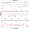 |
Fig. 1 Example of a RSG spectrum observed with WINERED: namely that of Betelgeuse in the Y band (echelle orders 57-52). Black thick lines show the reduced spectrum of Betelgeuse, after telluric lines were removed. Gray thin lines show the spectrum of the corresponding telluric standard A0V star, HIP 27830, after the stellar lines were removed. Red thick vertical dashed lines near the top edge of each panel indicate the wavelengths of the lines from the VALD3 and/or MB99 line list used for measuring [X/H]. Light-red thin vertical dashed lines indicate the wavelengths of the candidate lines preselected in Sects. 3.3 and 3.6 from VALD3 and/or MB99 but eventually rejected in Sects. 3.5.2 and 3.6 for both line lists. |
3.3 Line selection for the abundance analysis
For the abundance measurements, we chose the atomic lines that are comparatively free from contamination from surrounding lines among all the neutral and first-ionized atomic lines in the VALD3 and MB99 line lists. We considered lines in wavelength ranges of 9760–10 860 Å for the Y band and 11 620–13 170 Å for the J band (Sect. 2). Since the MB99 list contains only the lines with the wavelengths longer than 10 000 Å, the spectra within 9760–10 000 Å were analyzed only with VALD3. We excluded the lines of carbon, nitrogen, and oxygen2, along with hydrogen and helium, because the CNO abundances had been adjusted in such a way that the synthesized CN spectra well reproduced the observed ones as we see later (Sect. 3.4). We note that during line selection, we assumed 12C/13C = 10 as the typical isotope ratio of carbon for RSGs (Hinkle et al. 1976; Milam et al. 2009; Fanelli et al. 2022) and used solar isotope ratios from Asplund et al. (2009) for the other elements.
In order to evaluate the amount of contamination for each atomic line, we considered synthesized spectra of a theoretical RSG, RSG3 defined in Table 3 of T21, having the solar metallic- ity and Teff = 3850 K. Specifically, we synthesized three types of spectra for RSG3 for the wavelength range around each line with different groups of lines: (1) All – all the atomic and molecular lines, (2) OneOut – all the lines except for the line of interest (see Fig. 3 in Kondo et al. 2019, for three examples of OneOut spectra), and (3) OnlyOne – only the line of interest. With these synthesized spectra, we first measured the depth dOnlyOne from unity in the wavelength λ0 of the line in OnlyOne, excluding the lines shallower than 0.03 for Fe I lines and 0.01 for the other species. Then, following Kondo et al. (2019), we computed two EWs  , where α indicates All or OneOut, around the line, as defined by
 (3)
(3)
where fAll(λ) and fOneOut(λ) indicate the synthesized spectra for All and OneOut, respectively, and c indicates the speed of light. In the computation, we considered two wavelength ranges (Δ1 and Δ2 corresponding to 40 and 80 km s−1, respectively). Both Δ1 and Δ2 were larger than those for red giants used by Kondo et al. (2019) considering that vmicro of RSGs are larger than those of red giants. With these EWs, we defined two indices β1 and β2 as
 (4)
(4)
The two indices measure the degrees of contamination by other lines in the core part of the line (β1 ) and in the continuum region (β2). We chose the lines with β1 < 0.5 and β2 < 1.0 to exclude the highly contaminated lines. Furthermore, we removed the lines around which either the hydrogen Paschen series nor Helium 10 830Å lines is present within ±60 km s−1. We note that when two or more lines from an element were located within (Δ1 + Δ2)/2 = 60 km s−1, only the line with the largest dOnlyone was used.
Applying these criteria to our sample atomic lines left lines of Mg I, Si I, Ca I, Ti I, V i, Cr I, Fe I, Ni I, Zn I, Ge I, Sr II, Y II, and Zr I for VALD3 and Na I, Mg I,Al I, Si I, K i, Ca I, Ti I, Cr I, Fe I, Ni I, Sr II, and Y II for MB99. Especially, the criteria left 51 and 32 Fe I lines in the Y and J bands, respectively, for VALD3, and 42 and 30 lines for MB99. Fig. 3 shows log τRoss calculated with the RSG3 model as functions of some line parameters: excitation potential (EP), X index described in Sect. 3.5.2, dOnlyOne, EW, and reduced EW. We note that one of our line-selection conditions, log τRoss > −3, corresponds to log(EW/λ) ≲ −4.8 to −4.6 (or EW ≲ 150–350 mÅ), and the exact threshold depends mainly on the species (and wavelength) of interest.
Derived log g and related values.
3.4 Adjustment of the strengths of CN lines
Since YJ-band spectra of RSGs contain many CN lines, which contaminate the atomic lines of our interest for the abundance analysis, the difference in the strengths of CN lines between the observed and synthesized spectra, if exists, affects the chemical abundance measurements using atomic lines. The strengths of CN lines depend on two abundance ratios, [C/O] and [N/H], together with stellar parameters and metallicity (Appendix C). Since the two ratios affect the strengths of weak and strong CN lines differently, we optimized the two ratios, together with 12C/13C, for each star to well reproduce the observed CN strengths with synthesized ones for each of the VALD3 and MB99 line lists in the following procedure. We note that this process is simply for the purpose of adjusting the CN line strengths and is not intended for determining CNO abundances.
First, we chose the CN lines that are relatively free from contamination by lines of other species. For this, we synthesized two types of spectra, All and OnlyOne defined in Sect. 3.3, around all the CN lines listed by Sneden et al. (2014). We also synthesized another type of spectra named SameElIonOut (abbreviating same-element-ion-out) that is synthesized with the list of all the lines except for those of the species of interest, which is 12C14N, 13C14N, or 12C15N in this case. With these spectra, we defined two indices, β3 and β4, as
 (5)
(5)
 (6)
(6)
The two indices mimic β1 and β2 defined in Eq. (4), but they use the spectrum SameElIonOut instead of OneOut to measure the degree of contamination to a CN line by surrounding lines of species other than CN. Then, we imposed three criteria to filter out weak and/or heavily-contaminated 12C14N lines: dOnlyOne > 0.03, β3 < 0.3, and β4 < 0.3. We used the same conditions on the line depth dOnlyOne for 13C14N and 12C15N lines, but we relaxed the condition on the contamination fractions: β3 < 0.5, and β4 < 1.0. When two or more lines are located within 80 km s−1 (which is different from 60 km s−1 used for Fe I lines in Sect. 3.3), only the line with the largest dOnlyOne was used. Application of these criteria left 43 and 110 12C14N lines in the Y and J bands, respectively, for VALD3, and 49 and 133 lines for MB99. There are 5 and 6 13C14N lines left in the J band for VALD3 and MB99, respectively, to determine 12C/13C, and no 12C15N lines left for the both lists.
Fitting the selected CN lines simultaneously, we determined [C/O], [N/H], and 12C/13C together with the full-width at half maximum (FWHM) of the line broadening, vbroad, as functions of vmicro spanning 0.6–4.4 km s−1 with a step of 0.2 km s−1 for each star, as follows. We used small wavelength ranges (±Δ2/2 = ±40 km s−1) of the spectrum around the selected CN lines to fit with a synthesized one. Some ranges having unrealistic flux values caused by, e.g., poor continuum normalization, were excluded. For a given set of [C/O], [N/H], 12C/13C, and vbroad, we determined the constant continuum level of each range that minimized the residual between the observed and synthesized spectra. Then, we calculated the residual of pixels that appeared in any ranges. We determined [C/O], [N/H], 12C/ 13C, and vbroad that minimized the residual using SciPy package (Virtanen et al. 2020). We note that we assumed in the procedure the chemical abundances of all the elements other than carbon and nitrogen to be solar. Finally, we interpolated [C/O] [N/H], and 12C/ 13C on the vmicro set with a polynomial function and used the interpolated [C/O], [N/H], and 12C/13C as functions of vmicro together with the fixed [O/H] = 0.0 dex in the subsequent analyses for each star.
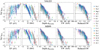 |
Fig. 3 log τRoss of the line-forming layers of the lines preselected in Sect. 3.3 as functions of the EP, the X index at 3850 K, the model depth dOnlyOne , the model EW, and the reduced model EW. Top and bottom panels show the results with employed line lists of VALD3 and MB99, respectively. The vertical error bar represents the range of Rosseland-mean optical depth where the contribution function for the line is larger than the half of the maximum value at log τRoss. Horizontal black dashed line at log τRoss = −3.0 indicates the final criteria of our line selection. |
3.5 Microturbulence (vmicro) and metallicity ([Fe/H])
In this section, we describe our procedure to determine vmicro and [Fe/H] simultaneously with the fitting of individual Fe I lines listed in Table D.3. We mainly follow the procedure given by Kondo et al. (2019) and Fukue et al. (2021), who analyzed the spectra of two K-type red giants, Arcturus and µ Leo, observed with the WINERED spectrograph, though we modified the procedure in many points in order to fit it to analyze RSGs.
3.5.1 Metallicity measurement with individual lines
For each Fe I line selected in Sect. 3.3 of a star, we estimated the metallicity, [Fe/H], with which the synthesized spectrum reproduced a small part of an observed spectrum around the line. The wavelength range with a width of Δ2 = 80 km s−1 (i.e., ±40 km s−1 from the wavelength λ0 of the line) was used to fit each Fe I line. During the fitting, we fixed Teff and log 𝑔 at the respective values determined in Sects. 3.1 and 3.2 and [C/H], [N/H], and [O/H] at those determined in Sect. 3.4. In contrast, we varied vmicro from 1.0 km s−1 to 4.0 km s−1 with a step of 0.1 km s−1 , and we then examined the dependence of the derived [Fe/H] on vmicro to determine the appropriate vmicro value.
The basic algorithm of our fitting procedure implemented in OCTOMAN followed that of Takeda (1995b); its detailed process is described in Appendix B. Briefly, we fitted the observed spectrum with a synthesized one until the end condition was satisfied, allowing four parameters to vary in an iterative way: the metallicity [Fe/H], FWHM vbroad of the line broadening under the assumption of a Gaussian profile, velocity offset ARV, and continuum normalization factor C. The end condition is met, if the variation of the fitting parameters is below a certain threshold. If the condition was not satisfied within 40 iterations, we considered the fitting for the line of the star a failure.
For each fitting run to converge well, the choice of the initial values for the free parameters (for a line) in the fitting matters. To determine the initial parameter set, we first examined a specific case of vmicro = 2.5 km s−1 among the above-mentioned set of vmicro . With the vmicro value, we tried to run the fitting procedure with nine sets of the initial parameters; three values for [Fe/H], −0.3, 0.0, and +0.3 dex, three values for vbroad, 14, 17, and 20 km s−1, and ARV = 0 km s−1. Then, we selected the parameter set that gave the smallest residual as the initial parameter set for vmicro = 2.5 km s−1. We subsequently gave as the initial parameter set for each of the vmicro grid points the bestfitting parameter set at the closest vmicro with which fitting had been successfully performed.
Applying the algorithm to the spectra of all of our observed RSGs, we obtained [Fe/H] as a function of vmicro spanning 1.0– 4.0 km s−1 for each line of each star.
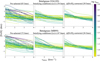 |
Fig. 4 Examples of how [Fe/H] is determined from each absorption line as a function of vmicro : here for the case for Betelgeuse. Top and bottom panels show the results with VALD3 and MB99, respectively. Left panels show the measurements for all the Fe I lines preselected in Sect. 3.3, and middle panels do for the lines satisfying conditions (i)–(v) in the main text (Sect. 3.5.2) and eventually used. Right panels show the measurements after the correction term Δ[Fe/H]i defined in Eq. (8) subtracted. Each curve in the figures corresponds to each absorption line color-coded according to log τRoss of the line-forming layer of the line; a lighter color corresponds to a larger log τRoss and thus a smaller EW. The dot on each curve indicates the [Fe/H] value determined with the corresponding vmicro . No dots are plotted where the fitting for a line with a value of vmicro failed. |
3.5.2 Simultaneous determination of vmicro and [Fe/H]
Using a series of [Fe/H] as functions of vmicro for all the analyzed lines of a star, we searched for the combination of vmicro and [Fe/H] that gives no correlation between line strength and [Fe/H] determined through the fitting of individual lines. Our search took four step: (1) excluding poorly-fitted lines, (2) setting the initial guess of vmicro and [Fe/H], (3) estimating and subtracting the correction term to [Fe/H] of each line, and (4) determining the final vmicro and [Fe/H].
In the first step, we examined how [Fe/H] was distributed against the set of vmicro for all the 83 (VALD3) and 72 (MB99) Fe I lines selected in Sect. 3.3 for each star, with the aim of excluding some lines that are unsuitable to the abundance analysis for the star. Left panels in Fig. 4 show the results for Betelgeuse as an example. Though [Fe/H] of each absorption line was expected to be a smooth function of vmicro , some of them showed anomalous variations. Furthermore, we failed to determine [Fe/H] with a considerable number of the vmicro values for some lines. These problems mainly occurred when the line was severely contaminated with other lines. In order to filter out undesirable lines due to these or some other reasons, we set five conditions for a line to be accepted. The first and second ones are that (i) [Fe/H] were successfully determined with more than 26 among 31 vmicro values, and (ii) all the slopes between the adjacent vmicro values are within a range from −2.0 dex (km s−1)−1 to +0.1 dex(km s−1)−1. These two conditions were imposed to filter out the lines that show anomalous variations. Remaining data gaps, if exist, were filled by means of linear interpolations (or extrapolations). The third one is that (iii) the Rosseland- mean optical depth log τRoss that gives the largest contribution function for the line (Gurtovenko & Sheminova 2015) satisfies log τRoss > −3.0. This condition was required because strong lines were often highly affected by non-LTE effects and imperfect modeling of damping wings (see Sect. 5.2 in Kondo et al. 2019). Indeed, as we show below, the [Fe/H] of strong lines that did not meed Condition (iii) tend to be larger than those of the weak lines by ~1 dex (see top-right panels of Figs. 5 and 6). The forth one is that (iv) the median value of [Fe/H] among all the vmicro values is between −1.5 and +1.0 dex. This condition was required because there was a disagreement between [Fe/H] and [M/H] in our spectral synthesis when [Fe/H] < −1.55 or [Fe/H] > +0.95 dex, as mentioned in Appendix B. Furthermore, the lines that fail to satisfy it, i.e., those with a very high or low [Fe/H], would be totally unexpected, which would be attributed to a poor match between the observed and synthesized spectra. The fifth, and final one is that (v) the median value of [Fe/H] among all the vmicro values is within 3σ of the median values of all the remaining lines for the star. Applications of the five conditions filtered our ∼30 and ∼20 lines for the VALD3 and MB99 lists, respectively, though the exact number of lines varied slightly, depending on the star. Middle panels of Fig. 4 show example results of the line fitting after the five conditions were imposed. As expected, the figure shows only lines with smooth relations between [Fe/H] and vmicro, without very high or low [Fe/H] values, and with weak or moderate line strengths.
From the remaining lines, we further excluded those that were accepted for fewer than nine out of ten stars; that is, we used the lines that were unusable for only zero or one stars. The excluded lines were not used in the subsequent analysis for all the stars together with the lines that were rejected for each star. The resultant number Nline of the lines to be used was 38 for VALD3 and 36 for MB99.
In the second step in the search for the vmicro and [Fe/H] combination, we determined the tentative values of vmicro and [Fe/H] of each star with the method described in Kondo et al. (2019). Briefly, we searched for the vmicro value that gives no correlation between the X index (Magain 1984) indicating the line strength and [Fe/H]. In general, evaluating the line strength from observed spectra of RSGs is not straightforward due to the severe line contamination. In the long-established abundance analysis of optical spectra of late-type giants and dwarfs without severe line contamination, the strength of each line is evaluated with either the observed or expected EW. The systematic errors in the resultant abundances depending on the choice of the two types of EWs have been extensively examined (e.g., Magain 1984; Mucciarelli 2011; Hill et al. 2011). In the case of either spectra of RSGs or NIR spectra of late-type stars (including RSGs), however, most of the lines to be used for abundance analysis are more or less contaminated by other lines, and thus it is usually difficult to accurately measure EWs observationally. We thus used, instead of observed EWs, the so-called X index in our analysis. The X index is often adopted for the abscissa of the curve- of-growth (e.g., Gray 2008). Kondo et al. (2019) successfully applied it in the analysis of NIR spectra of red giants. The X of each line in a spectrum is defined as
 (7)
(7)
where Θexc is the inverse temperature of the atmosphere layer from which the line originates. We adopted an approximation formula of Θexc = 5040 K/(0.86 Teff) following the work by Gratton et al. (2006). We note that the target type of stars analyzed by Gratton et al. (2006) was metal-rich red clump stars and thus different from ours, solar-metallicity RSGs. We also note that the value of ΘexcTeff is not a constant as we assume and depends on the line and/or spectral type of the star (Gray 2008). Nevertheless, we consider that the same formula should be applicable because the skewed X scale as a result of the variation of Θexc Teff would not change vmicro that gives no correlation between X and [Fe/H] of individual lines.
Here we describe the detailed procedure for the second step. For each star, we first prepared 106 bootstrap samples of the chosen lines, that is, we resampled the lines randomly from the original list of lines, allowing each line to be selected more than once. Then, for each bootstrap sample, the relation between the X index indicating the line strength and [Fe/H] for each vmicro was fitted with a linear regression function, [Fe/H] = a(vmicro)X + b(vmicro). The slopes of the regression lines, a(vmicro), were linearly interpolated to determine the microturbulent velocity vmicro,0 that gives a(vmicro,0) = 0 dex dex−1. The corresponding [Fe/H] value, b(vmicro,0) = [Fe/H]0, was also obtained with the linear interpolation of b(vmicro). Then, we considered the medians of [Fe/H]0 and vmicro,0 among the entire bootstrap samples as the best estimates of [Fe/H] and vmicro , respectively, of the star at this step. Finally, we calculated the 15.9% and 84.1% percentiles, i.e., 1σ intervals for a Gaussian distribution, of the bootstrap samples as the standard errors of the best estimates.
The determined [Fe/H] for most of the stars had a scatter of 0.3–0.4 dex; the middle panels of Fig. 4 show an example case. A significant amount of the large scatter was likely to be attributed to errors in log 𝑔 f (Andreasen et al. 2016; Kondo et al. 2019), and the systematic error in the line fitting originating in the line contamination. The two types of probable sources of errors are expected to add systematic errors to the [Fe/H] measurements for all the stars for each line. Thus, in the third step in the search for the vmicro and [Fe/H] combination, we took an approach similar to the differential analysis (Ramírez et al. 2014; Nissen & Gustafsson 2018), as we describe in the following two paragraphs, to remove this type of systematic errors.
In the usual differential analysis, [Fe/H] of individual lines of a target star are compared with those of a standard star, such as the Sun. Then, the offsets in [Fe/H] between the two stars are used to determine the differential metallicity (and some of the stellar parameters) of the target. In our case, however, none of the target stars had [Fe/H] measurements for all the lines of interest. Furthermore, none of the targets had a well-known [Fe/H] to be used as a standard star. Thus, the above-mentioned standardstar method was unsuitable in our derivation of the abundances. Instead, we calculated a “correction term” (or “line-by-line systematics”) to [Fe/H] of each line, using all the available [Fe/H] measurements for the targets, and used it. Specifically, we calculated the correction term Δ[Fe/H]i for line i, using [Fe/H] of the line i of each star n with vmicro,0 , which is denoted as ![$[{\rm{Fe}}/{\rm{H}}]_i^{(n)}$](/articles/aa/full_html/2025/01/aa52392-24/aa52392-24-eq32.png) , as
, as
![$\Delta {[{\rm{Fe}}/{\rm{H}}]_i} = {1 \over {{N_i}}}\mathop \sum \limits_{n = 1}^{{N_i}} \left( {[{\rm{Fe}}/{\rm{H}}]_i^{(n)} - [{\rm{Fe}}/{\rm{H}}]_0^{(n)}} \right),$](/articles/aa/full_html/2025/01/aa52392-24/aa52392-24-eq33.png) (8)
(8)
where Ni indicates the number of the stars having the [Fe/H] measurement for line i. We then “corrected” or removed the line-by-line systematic from ![$[{\rm{Fe}}/{\rm{H}}]_i^{(n)}$](/articles/aa/full_html/2025/01/aa52392-24/aa52392-24-eq34.png) as
as ![$[{\rm{Fe}}/{\rm{H}}]_i^{(n)} \mapsto [{\rm{Fe}}/{\rm{H}}]_i^{(n)} - \Delta {[{\rm{Fe}}/{\rm{H}}]_i}$](/articles/aa/full_html/2025/01/aa52392-24/aa52392-24-eq35.png) . Middle and right panels of Fig. 4 show an example case before and after the correction, respectively.
. Middle and right panels of Fig. 4 show an example case before and after the correction, respectively.
In the fourth and final step in the search for the vmicro and [Fe/H] combination, we recalculated vmicro,0 and [Fe/H]0 along with their standard errors, using the same method employed for obtaining the tentative values but with the corrected [Fe/H] values for individual lines. The scatter in ![$[{\rm{Fe}}/{\rm{H}}]_i^{(n)}$](/articles/aa/full_html/2025/01/aa52392-24/aa52392-24-eq36.png) for each star was confirmed to be smaller than the scatter in |Δ[Fe/H]i| (Figs. 5 and 6). Accordingly, we conclude that the correction terms improved the precision in the determined [Fe/H] as expected.
for each star was confirmed to be smaller than the scatter in |Δ[Fe/H]i| (Figs. 5 and 6). Accordingly, we conclude that the correction terms improved the precision in the determined [Fe/H] as expected.
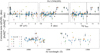 |
Fig. 5 Correction term to the determined [Fe/H] values for each line for VALD3 as functions of EP (top-left panel), X index at 3850 K (top-middle), log τRoss (top-right), and wavelength in the standard air (bottom). Black dots show |
![$[{\rm{Fe}}/{\rm{H}}]_i^{(n)} - [{\rm{Fe}}/{\rm{H}}]_0^{(n)}$](/articles/aa/full_html/2025/01/aa52392-24/aa52392-24-eq30.png)
3.6 Abundances of elements other than iron
Having determined Teff , log 𝑔, CNO abundances, vmicro , and [Fe/H] in previous sections, we determined the chemical abundances of elements other than iron. We used basically the same procedure as we had determined [Fe/H], but with some modifications.
For each line selected in Sect. 3.3 of an element X, we derived the abundance [X/H] for a parameter set of vmicro ranging from 1.0 to 4.0 km s−1 with a step of 0.1 km s−1, using the OCTOMAN code in the same way as for the iron abundance (see Sect. 3.5.1). During the fitting for the element X, we fixed the global metallicity [M/H] of the model atmosphere and the abundances of elements other than C, N, O, and X to the value of [Fe/H] that we had determined, and allowed [X/H], vbroad, ∆RV, and continuum normalization C to vary. After the fitting for the entire set of vmicro , we excluded the lines failing to satisfy any of the Conditions (i)–(iv) that had been applied in determining the iron abundance in Sect. 3.5.2. Then, we interpolated the set of vmicro and derived the abundance of an element X for a given line with vmicro,0.
We then calculated the correction term ∆[X/H]i for each line in the same way as for the iron abundance, subtracted the correction term from ![$[{\rm{X}}/{\rm{H}}]_i^{(n)}$](/articles/aa/full_html/2025/01/aa52392-24/aa52392-24-eq37.png) , and calculated the mean of [X/H] of all the remaining lines. Consequently, we have determined the abundances of Mg I, Si I, Ca I, Ti I, Cr I, Ni I, and Y II for VALD3 and Na I, Mg I, Al I, Si I, K I, Ca I, Ti I, Cr I, Ni I, and Y II for MB99.
, and calculated the mean of [X/H] of all the remaining lines. Consequently, we have determined the abundances of Mg I, Si I, Ca I, Ti I, Cr I, Ni I, and Y II for VALD3 and Na I, Mg I, Al I, Si I, K I, Ca I, Ti I, Cr I, Ni I, and Y II for MB99.
3.7 Error budget for abundance measurements
3.7.1 Error budget for [Fe/H]
We consider two sources of errors in the derived [Fe/H] of each star: (1) ∆b – the confidence interval in the determination of [Fe/H] and vmicro in the bootstrap and (2)  and
and  the errors propagated from the errors in Teff and log g, respectively. The total error ∆total in the final [Fe/H] measurement were calculated as
 (9)
(9)
In more detail, ∆b was estimated using the bootstrap method as described in Sect. 3.5.2. The error includes both the standard error due to the scatter in [Fe/H] determined for individual lines and the error propagated from the error in vmicro because we determined [Fe/H] and vmicro simultaneously with the bootstrap method. To determine ∆Teff with numerical error propagation for each star, we fitted again all the lines used for the final [Fe/H] determination, totaling 38 and 36 lines for VALD3 and MB99, respectively, with the determined vmicro and with three different effective temperatures assumed: the best estimate Teff , and the best estimate plus or minus its error, Teff ± ∆Teff . Then, we estimated the error ∆Teff by calculating the bootstrapped median of the differences between ![$[{\rm{Fe}}/{\rm{H}}]_i^{(n)}\left( {{T_{{\rm{eff}}}} \pm {\rm{\Delta }}{T_{{\rm{eff}}}}} \right)$](/articles/aa/full_html/2025/01/aa52392-24/aa52392-24-eq41.png) and
and ![$[{\rm{Fe}}/{\rm{H}}]_i^{(n)}\left( {{T_{{\rm{eff}}}}} \right)$](/articles/aa/full_html/2025/01/aa52392-24/aa52392-24-eq42.png) . We estimated the error ∆log 𝑔 in the same way.
. We estimated the error ∆log 𝑔 in the same way.
3.7.2 Error budget for [X/H] other than [Fe/H]
We consider two sources of errors in [X/H] of each star: (1) ∆′sca3 – the standard error of the line-by-line scatter and (2)  ,
, , and ∆′[Fe/H] – the errors propagated from the errors in vmicro, Teff, log g, and [Fe/H], respectively. Ignoring covariance terms, the total errors
 ![$\Delta '_{{\rm{total}}}^{[{\rm{X}}/{\rm{H}}]}$](/articles/aa/full_html/2025/01/aa52392-24/aa52392-24-eq47.png) in the final [X/H] was calculated as
in the final [X/H] was calculated as
![$\Delta _{{\rm{total}}}^{\prime [{\rm{X}}/{\rm{H}}]} \equiv \sqrt {\Delta {{_{{\rm{sca}}}^\prime }^2} + \Delta _{\upsilon _{{\rm{micro}}}^\prime }^\prime + \Delta {{_{{T_{{\rm{eff}}}}}^\prime }^2} + {{\Delta '}_{\log \,}}^2 + {\Delta _{[{\rm{Fe}}/{\rm{H}}]}}^2} .$](/articles/aa/full_html/2025/01/aa52392-24/aa52392-24-eq48.png) (10)
(10)
In more detail, ∆′sca was simply calculated as the standard error of [X/H] from individual lines for the elements where the number of the lines  for the element X for the star n is 5 or larger. In cases where
  is smaller than 5, however, the standard error of the [X/H] values is inaccurate, and thus, we multiplied the standard deviation of the measured [Fe/H] values by
  to estimate ∆′sca, assuming that the errors in [X/H] and [Fe/H] measurements from individual lines are approximately equal. The other error terms were estimated with numerical error propagation in the same way as the estimation of the errors
  and ∆log 𝑔 of [Fe/H]. We also determined the total error in [X/Fe] in a similar way.
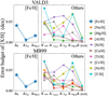 |
Fig. 7 Error budget of [X/H] measurements. Left panels show the medians of the absolute values of the three sources of errors (∆b , |


4 Chemical abundance analysis: Results
We summarize the resultant stellar parameters and [Fe/H] of the target RSGs in Table 3 and the chemical abundances in Tables D.1 and D.2. The typical precision ∆total in the determined [Fe/H] is ∼0.05 dex, which is dominated by ∆b in most cases (left panels of Fig. 7). This level of precision is comparable with, or better than, the previous works of RSGs mentioned in Sect. 1. The errors ![$\Delta '_{{\rm{total}}}^{[{\rm{X}}/{\rm{H}}]}$](/articles/aa/full_html/2025/01/aa52392-24/aa52392-24-eq53.png) in the determined [X/H] other than [Fe/H] are dominated by ∆sca for most of the elements, especially the elements with a small number of measured lines (right panels of Fig. 7). Considering the high sensitivity of [X/H] on Teff and log g for some of the elements, especially, [Si/H], [Ni/H], and [Y/H], the high precision of Teff and log g in this work (~30−100 K for Teff and ~0.1−0.3 for log g) is essential for the high precision in the [X/H] measurements.
in the determined [X/H] other than [Fe/H] are dominated by ∆sca for most of the elements, especially the elements with a small number of measured lines (right panels of Fig. 7). Considering the high sensitivity of [X/H] on Teff and log g for some of the elements, especially, [Si/H], [Ni/H], and [Y/H], the high precision of Teff and log g in this work (~30−100 K for Teff and ~0.1−0.3 for log g) is essential for the high precision in the [X/H] measurements.
In this section, we evaluate the results with VALD3 and MB99. As we demonstrate in this section, both the results turn out to be similar in terms of the precision and systematic bias, and thus we conclude that the two results are equally reliable.
Derived stellar parameters and [Fe/H].
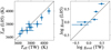 |
Fig. 8 Comparison of our results and those of Levesque et al. (2005) for the RSGs included in both samples: Teff and log 𝑔. |
4.1 Direct comparison with previous results
Some previous works determined the stellar parameters and/or chemical abundances of the ten RSGs that we analyzed in this paper. In this section, we compare our results with previous measurements.
Figure 8 compares Teff and log g in this work with those determined by Levesque et al. (2005). Levesque et al. (2005) determined Teff of all our ten target RSGs, but they only determined log g of five RSGs among them (V809 Cas, V424 Lac, TV Gem, BU Gem, and NO Aur). We find that the difference in our results of Teff and theirs are smaller than 100 K, which is almost within the error bars (see the detailed discussion in Sect. 4.2 of T21). We also find a good agreement between our results of log g and theirs, which is expected, given that Levesque et al. (2005) and we used similar methods in determining log g. These consistencies support the reliability of our Teff and log g measurements.
Figure 9 compares stellar parameters and [Fe/H] in this work and those determined by Luck & Bond (1980) and Luck (1982a,b) and summarized by Luck & Bond (1989). Our and their samples include eight common RSGs (ζ Cep, 41 Gem, ξ Cyg, V809 Cas, V424 Lac, TV Gem, BU Gem, and NO Aur). The comparison reveals large differences in the derived stellar parameters, especially in Teff and vmicro, which might be attributed to differences in the derivation methods and the model atmospheres employed; the procedure employed by Luck & Bond (1989) was based on EW measurements of individual lines in the optical. There is no simple way to determine which one of the two results is more accurate. Nevertheless, at least, our determined Teff and log L are in good agreement with a stellar evolution model by Ekström et al. (2012) (see Sect. 4.3 of T21). Moreover, the dependence of the correction term Δ[Fe/H]i on EP is consistent with zero for both VALD3 and MB99 line lists: +0.004 ± 0.028 and +0.042 ± 0.025 dex/eV, respectively (topleft panels of Figs. 5 and 6). In other words, our Teff values determined using the LDR method, and thus independent of the abundance measurement through the line fitting, satisfy the condition known as the excitation equilibrium (e.g., Jofré et al. 2019). These facts reassure for the accuracy of our result. In the next section, we further use some well-established relations to discuss the reliability of our abundance analysis results.
4.2 Validation of the abundance analysis results
In this section, we validate our results on two points: (i) the relation between log g and vmicro (Sect. 4.2.1), and (ii) comparison with the Galactic radial metallicity/abundance gradients traced with Cepheids (Sects. 4.2.2 and 4.2.3, respectively).
4.2.1 Relation between log g and vmicro
We show the relation between log g and vmicro in Fig. 10 to examine the reliability of our determined vmicro values, which affects the resultant abundances. It is known that vmicro can be, in general, approximated by a function of log g and some additional parameters (e.g., Holtzman et al. 2018). Indeed, Fig. 10 shows an overall (negative) correlation between log g and vmicro that we derived for our target RSGs in both the results with the VALD3 and MB99 line lists. Moreover, log g and vmicro of the RSGs obtained in this work and red giants obtained in a previous work (Heiter et al. 2015) seem to form a continuous relation over a large log g range even though there is no guarantee that RSGs and red giants follow a single log g–vmicro relation. With these results, we conclude that there is no evidence of an apparent systematic bias in our vmicro determination.
We then compare the relation between log g and vmicro with those in literature. Figure 10 overlays three relations from literature: one calibrated and used by Holtzman et al. (2018) for APOGEE DR13, one calibrated using observational samples of vmicro measurements by Adibekyan et al. (2012), and one calibrated using the CIFIST grid of 3D hydrodynamic models (Ludwig et al. 2009) by Dutra-Ferreira et al. (2016). We note that the second among the three relations was used by Alonso- Santiago et al. (2017) and the third one by Alonso-Santiago et al. (2018, 2019) and Negueruela et al. (2021) to estimate vmicro of RSGs. We find an overall agreement between our results and the previously-reported three relations around −0.5 ≲ log g ≲ 0.5. Nevertheless, some systematic differences are present between the relations. The differences might be attributed to the fact that the previously-reported relations are not optimized for the log g range of RSGs. Indeed, the covered ranges for the stellar parameters of the calibrating samples are 3 < log g < 5 and 4500 < Teff < 6500 K for the work by Adibekyan et al. (2012) and 2.5 ≤ log g ≤ 4.5 and 4400 < Teff < 6500 K for that by Dutra-Ferreira et al. (2016). The sample of APOGEE DR13 covers a wider range, −0.5 < log g < 3.8, which include the log g range of RSGs; nevertheless their sample is mostly concentrated in a relatively narrow range 1.5 ≲ log g ≲ 3.5 (Fig. 6 of Holtzman et al. 2018). Thus, the relation for APOGEE DR13 for lower log g stars may have considerable systematic uncertainty. In fact, the stars in the APOGEE DR14 (Holtzman et al. 2018) with Teff and log g comparable with those of our target RSGs (Teff ≲ 4000 K and log ≲ 0.5 dex) have vmicro > 2.0 km s−1. These vmicro values are inconsistent with the log g–vmicro relation that was adopted for APOGEE DR13 but are consistent with the vmicro values of RSGs determined here. A grid of 3D hydrodynamic models for RSGs is required to examine further the reliability of the estimated vmicro , which is beyond the scope of this work.
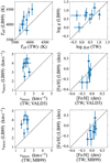 |
Fig. 9 Comparison of our results and those of Luck & Bond (1989) for the RSGs included in both samples: stellar parameters and [Fe/H]. Top panels show Teff and log g, which are used in common with VALD3 and MB99. Middle and bottom panels show vmicro and [Fe/H] determined with VALD3 and MB99, respectively. |
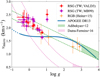 |
Fig. 10 Relation between log g and vmicro . Red closed circles and magenta closed squares indicate the values that we determined for the target RSGs with VALD3 and MB99, respectively. Orange open circles indicate the values for the five solar-metallicity red giants among the Gaia FGK benchmark stars (Heiter et al. 2015) used in T21. Blue solid lines show the relation used in the ASPCAP code for APOGEE DR13 (Holtzman et al. 2018) for the log g ranges of their calibrating sample, with the extrapolated relation indicated by blue dotted lines. Green and pink dashed lines indicate the relations calibrated by Adibekyan et al. (2012) and Dutra-Ferreira et al. (2016), respectively, for Teff = 3500 and 4000 K, with the log g ranges of their calibrating samples indicated by shades in the respective colors. |
4.2.2 Radial metallicity gradient compared with Cepheids
In this section and the next section, we compare the chemical abundances of RSGs with those of another type of young stars, Cepheids. Ideally, we should compare the abundances of RSGs and Cepheids in a single cluster to ensure that both objects have a common abundances. However, the number of clusters encompassing RSGs and Cepheids (e.g., Negueruela et al. 2020; Alonso-Santiago et al. 2020) is rather limited. Thus, instead, we have compared the derived chemical abundances of RSGs with the radial abundance gradients traced with Cepheids using the abundance measurements presented by Luck (2018). Considering the young ages of RSGs (≲50 Myr) and Cepheids (≲300 Myr), the abundances of both RSGs and Cepheids are expected to follow the common gradients, assuming that there is no mechanism favoring the formation of low- or high-metallicity RSGs and/or Cepheids. In fact, Esteban et al. (2022) demonstrated that some of the young objects in the solar-neighborhood (H II regions, B-type stars, classical Cepheids, and young open clusters) have the metallicity consistent with each other within 0.1 dex.
Figure 11 plots the metallicities of our target RSGs obtained in this work, along with the metallicities of Cepheids reported by Luck (2018) as a function of the Galactocentric distance RGC . Also shown are some of the metallicity measurements of RSGs in star clusters or star-forming complexes from previous works (Alonso-Santiago et al. 2017, 2018, 2019, 2020; Negueruela et al. 2021; Gazak et al. 2014; Fanelli et al. 2022), as we focus on RSG clusters in forthcoming papers. We calculated the RGC values of all the plotted objects assuming the distance to the Galactic Center of R⊙ = 8.15 kpc (Reid et al. 2019), which is different from 7.9 kpc adopted by Luck (2018) for gradient calculations. Accordingly, we recalculated the radial metallicity gradient of Cepheids, after five iterations of three- sigma clipping, using the [Fe/H] values reported by Luck (2018) and the Bayesian distance estimates using the Gaia DR2 parallax data by Bailer-Jones et al. (2018) with excluding some stars: those with negative Gaia DR2 parallaxes following Luck (2018), five stars (HK Cas, BC Aql, QQ Per, EK Del, and EQ Lac) as recommended by Luck (2018), and SU Cas as recommended by Kovtyukh et al. (2022) and Matsunaga et al. (2023). We also note that we rescaled the [Fe/H] values presented in the previous works to the solar abundances reported by Asplund et al. (2009), when the differential analysis against the solar spectrum might not have been performed.
Consequently, we find a good agreement between [Fe/H] of the RSGs that we obtained using MB99 and those of Cepheids; the difference in the gradients between the two is 0.004 dex. In contrast, [Fe/H] of the RSGs obtained using VALD3 is slightly, by 0.125 dex, smaller than those of Cepheids. This level of discrepancy is as expected given the difference in the log g f values in the two line lists (see Fig. 7 in Kondo et al. 2019). In fact, analyzing NIR YJ-band spectra of two red giants, Arcturus and µ Leo, Kondo et al. (2019) found that [Fe/H] of the two stars determined with the MB99 list were well consistent with literature values, but [Fe/H] using VALD3 were smaller than those using MB99 by 0.20 and 0.11 dex for Arcturus and µ Leo, respectively. These consistencies support the reliability of our [Fe/H] measurements, especially when using the MB99 list, indicating that our [Fe/H] measurements should be accurate within ∼0.1 dex.
In contrast, [Fe/H] of RSGs determined by some previous works among those plotted in Fig. 11 (Alonso-Santiago et al. 2018, 2019, 2020; Negueruela et al. 2021; Fanelli et al. 2022) are found to be systematically lower than those of Cepheids by 0.2–0.3 dex. Such low [Fe/H] values have been often found in cool giants with low log g (e.g., Casali et al. 2020; Magrini et al. 2023; Gaia Collaboration 2023a). A part of the systematic differences, especially of Fanelli et al. (2022), could possibly be explained with the vmicro values that they adopted, as discussed below, considering the strong degeneracy between [Fe/H] and vmicro.
We show in Fig. 12 vmicro adopted by this work and the previous works cited in Fig. 11 to highlight their differences to help understand the discrepancies in [Fe/H] among the works in conjunction with vmicro . Our vmicro (TW in the figure) are found to be concentrated at around ∼2 km s−1 and are similar to those reported by Alonso-Santiago et al. (2017, 2018, 2019, 2020) and Negueruela et al. (2021) (designated as A17, A18, A19, A20, and N21, respectively, in the figure). In contrast, those reported by Gazak et al. (2014) and Fanelli et al. (2022) (G14 and F22, respectively) are significantly higher than our values.
In the work by Fanelli et al. (2022) among those cited in Fig. 12, they analyzed optical and NIR spectra of RSGs in the Perseus Complex. We find that their resultant [Fe/H] are systematically ~0.3 dex lower than the metallicity gradient of Cepheids (squares in Fig. 11), and we discuss here its possible connection to the vmicro values that they adopted. They adopted vmicro of ~ 1 km s−1 higher than ours, maybe because they included strong Fe I lines in their analysis; they used Fe I lines having −4 ≲ log τRoss ≲ −1, as opposed to our line-selection criterion of log τRoss > −3. Their larger vmicro could result in a ~0.2−0.4 dex smaller [Fe/H] than ours. In fact, recalculation of vmicro of our target RSGs with the criteria of log τRoss > −4 instead of −3 yields an increase in vmicro by ~0.8 and 0.3 km s−1 for VALD3 and MB99, respectively, which results in [Fe/H] smaller by ~0.18 and 0.06 dex, respectively. This positive systematic bias in vmicro is caused by the large positive systematic errors in the measured [Fe/H] of strong lines (log τRoss < −3) as shown in the top right panels of Figs. 5 and 6. The difference in the Teff values could also in part contribute to the difference in the resultant [Fe/H], but it would be smaller because the sensitivity of [Fe/H] to Teff is low:  dex/100K (See ΔTeff in the left panels of Fig. 7).
In the work by Alonso-Santiago et al. (2017, 2018, 2019, 2020) and Negueruela et al. (2021) among those cited in Fig. 12, they analyzed optical spectra of RSGs in some young clusters (NGC 6067, NGC 3105, NGC 2345, NGC6649, NGC 6664, and Valparaiso 1). The resultant [Fe/H] of all these works except for the work by Alonso-Santiago et al. (2017) are systematically ~0.2−0.3 dex lower than the metallicity gradient of Cepheids (triangles in Fig. 11), although they used vmicro whose ranges are similar to ours (Fig. 12). Since most of their observed targets (spectral types between G–K) are warmer than our target RSGs (spectral types between K–early M) and also have larger log 𝑔, it is not trivial to identify the cause of the differences.
In the work by Gazak et al. (2014), which is the last one among those cited in Fig. 12, they obtained [Fe/H] of RSGs consistent with the metallicity gradient of Cepheids (diamonds in Fig. 11). Their spectra have relatively low resolution compared to those used in all the other works mentioned here. Furthermore, they determined global metallicity, using most of the lines appearing in the J band including atomic lines from elements other than iron, molecular lines, and/or strong lines. This is in contrast to our approach, which focuses solely on relatively weak Fe I lines to measure [Fe/H]. Given these methodological differences, we do not discuss the cause of the consistency here.
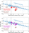 |
Fig. 11 Metallicities of RSGs compared with the radial metallicity gradient of Cepheids for the Galactocentric distance (RGC). Filled red circles (top panel) and filled magenta squares (bottom panel) show the derived [Fe/H] of our target RSGs for VALD3 and MB99, respectively. Blue dots show [Fe/H] of Cepheids (Luck 2018) within 5 < R < 14 kpc as an indicator of the radial metallicity gradient of young stars. Blue dashed lines show the linear fit to the Cepheids’s metallicities. Open brown symbols show the weighted-mean metallicities and their corresponding standard errors of RSGs in star clusters or star-forming complexes within 6 ≲ RGC ≲ 10 kpc measured by some previous works: Gazak et al. (2014) depicted with a diamond, Alonso-Santiago et al. (2017, 2018, 2019, 2020) and Negueruela et al. (2021) with triangles, and Fanelli et al. (2022) with a pentagon. |
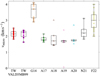 |
Fig. 12 Box plot of vmicro determined in this work (marked as TW) and previous works for RSGs plotted in Fig. 11: Gazak et al. (2014) as G14, Alonso-Santiago et al. (2017, 2018, 2019, 2020) as A17–A20, respectively, Negueruela et al. (2021) as N21, and Fanelli et al. (2022) marked as F22. |
4.2.3 Radial abundance gradients compared with Cepheids
Regarding chemical abundances of elements other than iron, we plot in Fig. 13 the weighted means of the derived [X/Fe] of our target RSGs after the radial abundance gradients of Cepheids are subtracted. The abundance gradients are calculated as is done for the metallicity gradient. As with the case for [Fe/H] discussed in the previous section, the abundance ratios [X/Fe] of both RSGs and Cepheids are expected to follow common gradients. Hence, the differences between them, which are plotted in the figure, would be zero when the abundance measurements for both RSGs in this work and Cepheids in the work by Luck (2018) are accurate. We note that sodium synthesized inside a star via the NeNa cycle can potentially appear on the surface of evolved stars through mechanism(s) such as dredge-up, rotation, and mass loss (El Eid 1994; Ekström et al. 2012; Smiljanic et al. 2016). Consequently, the current surface abundances of sodium, as well as carbon, nitrogen, and oxygen, of RSGs do not necessarily reflect their initial surface abundances, and by extension, the current surface abundances of Cepheids. In other words, the values plotted in Fig. 13 for Na I need not be zero.
Consequently, we find a good agreement (i.e., within ~0.1 dex) in the abundance ratio of the most representative α element, [Mg/Fe], along with some other elements (e.g., [Ca/Fe] and [Ni/Fe]). On the contrary, we find systematic offsets in the obtained abundances for some other species, most notably for [Si/Fe] and [Y/Fe] with offsets of ~0.3 dex. Discrepancies of this type were often seen in RSGs’ abundances reported by previous papers (open symbols in Fig. 13). The reason for the discrepancies is, however, unknown as of yet and is a remaining problem in the abundance analysis of RSGs.
In order to assess the possible impact of one of the shortcomings of our analysis, namely the LTE assumption, we derived non-LTE corrections for a part of the lines of Mg I, Si I, Ca I, Ti I, Cr I, and Fe I using the online tool developed by M. Bergemann’s group (Kovalev et al. 2019)4. The RSG3 model parameters (Table 3 of T21) and the RSG-MARCS grid of model atmospheres were employed in the test. For [Fe/H], we find that the non-LTE corrections for 34 out of 57 Fe I lines that were used for either VALD3 or MB99 can be calculated with the tool (Bergemann et al. 2012a, b), and all the corrections are negligible (≲ ±0.01 dex), indicating that the non-LTE effect does not affect our metallicity determination. Similarly, the non-LTE corrections for [Ca/H] and [Cr/H] are also negligible. For [Ca/H], 5 out of 6 Ca I lines have corrections (Mashonkina et al. 2007), and for [Cr/H], 10 out of 15 Cr I lines have corrections (Bergemann & Cescutti 2010), all of which were zero. In contrast, the non-LTE effect may affect [Mg/H], [Si/H], and [Ti/H]. For [Mg/H], the corrections can be calculated for 4 out of 5 Mg I lines (Bergemann et al. 2015, 2017): the corrections are zero for two lines (12417.937Å and 12433.45Å), −0.040dex for 12039.822 Å, and −0.312dex for 12083.65Å. The rather large correction for the last line, which was only used with the MB99 list, is consistent with the large ∆[X/H]i value for the line, +0.463 dex. We reiterate that a positive ∆ [X/H]i value corresponds to the observed line strength being higher than the synthesized one. For [Si/H] and [Ti/H], the corrections can be calculated for 14 out of 18 Si I lines (Bergemann et al. 2013) and 18 out of 25 Ti I lines (Bergemann 2011), with typical corrections of −0.17 and +0.11 dex, respectively. These may at least partly explain the abundance discrepancies of ~ + 0.3 dex for [Si/Fe] and ~−0.15 dex for [Ti/Fe]. In summary, while the non-LTE effect may not affect our abundance results of some elements (Fe I, Ca I, and Cr I), they may have a noticeable impact on some others (Mg I, Si I, and Ti I). Nevertheless, we dare not apply the non-LTE corrections to our measurements given the incomplete line list in the tool used. Further 3D non-LTE modeling of RSG spectra with a more complete line list is required to better understand the abundance discrepancies observed between RSGs and Cepheids.
Nevertheless, since most of the Galactic RSGs have stellar parameters within a certain small range (3500 ≲ Teff ≲ 3900 K and −9 ≲ Mbol ≲ −6; Levesque et al. 2005), we expect that the amount of the systematic error for a given element is nearly constant for any RSGs at least with solar metallicity, as far as the same abundance analysis method, the same line list, the same model atmosphere grid, and the same wavelength coverage is employed. To examine if the expectation is genuinely the case with our results, we calculated the weighted standard deviation (SD) of [Fe/H] and [X/Fe] among the ten RSGs after the radial abundance gradients of Cepheids are subtracted. These values basically represent the summations of the statistical and systematic errors in our abundance measurements (without systematic offsets included in the summations), assuming that the chemical abundance of RSGs for each element follows a tight abundance gradient. Tables D.1 and D.2 tabulate the calculated SDs. In consequence, we find that the dispersions are within 0.04–0.12 dex for the elements with the number of measured lines Nline larger than two ([Fe/H], [Mg/Fe], [Si/Fe], [Ca/Fe], [Ti/Fe], [Cr/Fe], and [Ni/Fe]). The other elements with a smaller Nline, [Na/Fe], [Al/Fe], and [Y/Fe], have the dispersion within 0.09–0.18 dex. These dispersions are consistent with the quoted errors, at least for most elements. This fact implies good reliability of our procedure of abundance measurement within the quoted error for the relative abundance difference between two objects, although the absolute abundance values for some elements still suffer a significant amount of systematic bias in general.
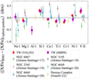 |
Fig. 13 Chemical abundances of RSGs after subtracting the radial abundance gradients of Cepheids. Filled red circles and filled magenta squares show the weighted mean and standard error of the derived [X/Fe] of our targets RSGs for VALD3 and MB99, respectively, after subtracting the radial abundance gradients of Cepheids, which are tabulated in Table D.2 as Mean. Open symbols show those for RSGs by the works measuring [X/Fe] as well as [Fe/H] among those cited in Fig. 11: Alonso-Santiago et al. (2017, 2018, 2019, 2020) with green, brown, pink, and cyan/blue triangles, respectively, and Fanelli et al. (2022) with yellow pentagons. We note that we show the results for all the elements for which we determined the abundances of RSGs, except for [K/Fe], as the abundance for Cepheids were not measured by Luck (2018). |
5 Summary and future prospects
In this paper, we establish a procedure for determining the chemical abundances of RSGs using NIR high-resolution spectra in the YJ bands. We tested the procedure through the analysis of NIR high-resolution spectra of ten nearby RSGs located within 8 ≲ RGC ≲ 10 kpc, which were obtained with the WINERED spectrograph (0.97–1.32 µm; R = 28 000). In our procedure, we first determined the effective temperature Teff, using LDRs of 11 Fe I–Fe I line pairs as in T21, and calculated the surface gravity log 𝑔 using the Stefan-Boltzmann law combined with Geneva’s stellar evolution model. We then determined the microturbulent velocity vmicro and the metallicity [Fe/H] simultaneously by fitting relatively isolated individual Fe I absorption lines. Finally, we fitted individual lines and determined the relative abundance of elements X to hydrogen [X/H] of Mg I, Si I, Ca I, Ti I, Cr I, Ni I, and Y II for the VALD3 and MB99 line lists, and in addition Na I, Al I, and K I for the MB99 list. We also estimated the relative precisions of the abundances using the standard deviations for the sample RSGs and found them to be 0.04–0.12 dex for the elements with a sufficient number of lines analyzed (e.g., Fe I and Mg I) and up to 0.18 dex for the elements with fewer than three lines analyzed (e.g., Na I and Y II).
Our procedure has advantages over previous works with regard to three main points: (1) the procedure is based on the fitting of observed spectra with synthesized ones on a line-by-line basis, as opposed to simple measurements of EWs as employed in some works, which allows us to circumvent the overestimation of abundances due to contamination by surrounding lines; (2) the procedure does not use molecular lines for determining stellar parameters, which allows us to circumvent effects related to the complicated outer atmospheres of RSGs; and (3) the procedure carefully adjusts [C/H], [N/H], and [O/H] to minimize potential systematic bias in the fitting of the lines of interest that originate in contaminating CN molecular lines.
We evaluated the reliability of our results in two ways. First, we compared the relation between log 𝑔 and vmicro with those derived from previous observational and theoretical results and found no apparent systematic bias in our derived vmicro values (Fig. 10). Second, we compared the radial abundance gradients of our sample RSGs with those of Cepheids in the literature (Figs. 11 and 13). We found good agreement (≲0.1 dex) for some abundances, notably [Fe/H] and [Mg/Fe], which are particularly useful abundances in the study of galactic chemical evolution. This result markedly differs from those of most previous works, reporting values of ~0.2–0.3 dex lower [Fe/H] than those of Cepheids. In contrast, we found discrepancies of as large as ~0.5 dex for some others, such as [Si/Fe], the cause of which may be related to a 3D non-LTE effect and/or uncertainty in the line list used, although were not able to come to any firm conclusions. Nevertheless, our procedure should be reliable with regard to its capacity to differentiate the abundances of two RSGs (or two groups of RSGs), considering that the standard deviation of the derived chemical abundances among our sample RSGs is comparable with the quoted precision in the measured abundances.
RSGs have extremely high luminosities (≳104L⊙), and hence they can be used as good tracers of the chemical abundances of young stars at large distances. Indeed, it is expected that we will be able to spectroscopically observe the brightest individual RSGs at a distance of ~1 Mpc, which is the distance to M31, with recently developed and/or near-future NIR high-resolution spectrographs with a very high throughput attached to large- aperture telescopes, such as WINERED/Magellan (Ikeda et al. 2022). Also, RSGs over a large area of the Galactic plane can be observed even with less-sensitive facilities, as long as the dust extinction to the target is not excessively severe. Mapping observations of these RSGs would be highly useful for studying the 2D distribution of the chemical abundances on the disks of the Milky Way and nearby galaxies, providing a means to constrain galactic chemical evolution theory.
Data availability
The abundance measurements and line list are available as Appendix D at Zenodo (https://doi.org/10.5281/zenodo.14286491). All the tables and reduced spectra are available at the CDS via anonymous ftp to cdsarc.cds.unistra.fr (130.79.128.5) or via https://cdsarc.cds.unistra.fr/viz-bin/cat/J/A+A/693/A163
Acknowledgements
We acknowledges useful comments from the referee, Alexander Ebenbichler. We are grateful to Yuki Moritani, Kyoko Sakamoto, Keiichi Takenaka, and Ayaka Watase for observing a part of our targets. We also thank the staff of Koyama Astronomical Observatory for their support during our observations. WINERED was developed by the University of Tokyo and the Laboratory of Infrared High-resolution spectroscopy (LiH), Kyoto Sangyo University under the financial supports of Grants-in-Aid, KAKENHI, from Japan Society for the Promotion of Science (JSPS; Nos. 16684001, 20340042, and 21840052) and the MEXT Supported Program for the Strategic Research Foundation at Private Universities (Nos. S0801061 and S1411028). This work has been supported by Masason Foundation. DT acknowledges the financial support from Toyota/Dwango AI scholarship, Iwadare Scholarship Foundation, and JSPS Research Fellowship for Young Scientists and accompanying Grants-in-Aid for JSPS Fellows (21J11555 and 23KJ2149). BT acknowledges the financial support from the Japan Society for the Promotion of Science as a JSPS International Research Fellow. BT acknowledges the financial support from the Wenner-Gren Foundation (WGF2022-0041). HS acknowledges the financial support by JSPS KAKENHI Grant Number 19K03917. This work has made use of the VALD database, operated at Uppsala University, the Institute of Astronomy RAS in Moscow, and the University of Vienna. This research has made use of the SIM- BAD database, operated at CDS, Strasbourg, France. This work presents results from the European Space Agency (ESA) space mission Gaia. Gaia data are being processed by the Gaia Data Processing and Analysis Consortium (DPAC). Funding for the DPAC is provided by national institutions, in particular the institutions participating in the Gaia MultiLateral Agreement (MLA). The Gaia mission website is https://www.cosmos.esa.int/gaia. The Gaia archive website is https://archives.esac.esa.int/gaia. This publication makes use of data products from the Two Micron All Sky Survey, which is a joint project of the University of Massachusetts and the Infrared Processing and Analysis Cen- ter/California Institute of Technology, funded by the National Aeronautics and Space Administration and the National Science Foundation.
Appendix A Spectral synthesis in OCTOMAN
For the spectral synthesis function in OCTOMAN, we wrapped the spectral synthesis code MOOG (Sneden 1973; Sneden et al. 2012)5. MOOG synthesizes spectra of late-type stars, assuming the 1D LTE with the plane-parallel geometry.
OCTOMAN provides users with some choices of the model atmosphere grid, including the ATLAS9 grids (Kurucz 1993; Castelli & Kurucz 2003; Mészáros et al. 2012) and the MARCS grids (Gustafsson et al. 2008). OCTOMAN obtains the exact model atmosphere for a given set of stellar parameters with linear interpolation (or extrapolation for log 𝑔 < 0) from the grid. In this paper, we used the MARCS spherical grid with M = 5 M⊙ and vmicro = 2 km s−1. When no model atmosphere was provided for a grid point with vmicro = 2 km s−1, we used vmicro = 5 km s−1 model instead. We note that the difference in the geometries between the radiative transfer code (plane-parallel) and the model atmosphere (spherical) only slightly affects the synthesized spectra in general (Heiter & Eriksson 2006).
The code provides three choices for the atomic line list: the third release of the Vienna Atomic Line Database (VALD3; Ryabchikova et al. 2015)6, the list of lines in 10 000–18 000 Å with astrophysical log 𝑔ƒ values constructed by Meléndez & Barbuy (1999, MB99), and the line list complied by R. Kurucz7.
The code considers lines of all the molecules included in the VALD3 database except for TiO. VALD3 contains lines of 12C1H, 13C1H, 14N1H, 12C2, 12C14N, 12C16O, 12C17O, 12C18O, 13C16O, and TiO in the YJ bands, among which 12C14N gives the largest contribution to the spectra of our target RSGs. A user can select whether to replace the line list of the 12C14N molecule from the VALD database with the list of 12C14N, 12C15N, and 13C14N calculated by Sneden et al. (2014). The difference in 12C14N between the two is small, but we found that some lines in the YJ bands only appear in the latter list8. Thus, we used the latter list in this paper.
The code provides three options for the line lists for metal oxides (e.g., TiO), where weaker lines are filtered out of the complete set of the known lines according to a set of threshold conditions, in which the “X index” at 3500 K defined in Eq. (7) is utilized. This constraint is set because the complete line lists of these molecules contain too many lines to synthesize. The three options are (i) the combination of 48Ti16O (X > −4.5), 51V16O (X > −3.0), and 90Zr16O (X > −3.5) line lists calculated by B. Plez9, (ii) the ExoMol line lists of 48Ti16O (X > −4.5), 46Ti16O, 47Ti16O, 49Ti16O, and 50Ti16O (X > −3.5) (McKemmish et al. 2019) and 51V16O (X > −4.0) (McKemmish et al. 2016), and (iii) basically identical to the second option but with a slight modification, adjusting log 𝑔ƒ values of TiO to better reproduce the observed spectra of RSGs by adding 0.3 dex to log 𝑔ƒ of the ϕ system (b1Π−d1Σ+) and subtracting 0.3 dex from log 𝑔ƒ of the δ system (b1Π−a1Δ). In this paper, we adopted the option (iii) to best reproduce the observed spectra of the RSGs.
In addition, the code adopts the line list of 56Fe1H calculated by B. Plez9. With extensive examination, we found that some lines of FeH appear in the YJ-band spectra of the RSGs with a depth of up to ~0.05 and that those lines are well reproduced by synthesized spectra with the dissociation energy of 1.59 eV (Schultz & Armentrout 1991).
Appendix B Fitting procedure for Fe I absorption lines in OCTOMAN
This section describes the detailed procedure to fit a Fe I absorption line implemented in the OCTOMAN code. In the analysis of fitting of lines of other species presented in this paper, we use mostly the same procedure. The procedure mainly follows the algorithm presented by Takeda (1995b) but with some modifications.
We consider the following four variables during the fitting for a line: (1) iron abundance, [Fe/H] (or the abundance of another element) – the parameter of interest, (2) FWHM (i.e., vbroad) of the line broadening including three components of vmacro, rotation, and instrumental broadening, (3) Velocity offset, ΔRV, and (4) Continuum normalization factor, C.
Related to variable (1), in the current work, we fix the abundances of carbon, nitrogen, and oxygen to the respective values determined in Sect. 3.4. We also fix the abundance values of the other elements to the iron abundance in determining [Fe/H]. We assume that the global metallicity [Μ/H] of the model atmosphere is equal to [Fe/H].
As for variable (2), the instrumental broadening in our observations (R = 28 000 for the Wide mode of WINERED) is comparable with or smaller than vmacro of RSGs (e.g., ~15 km s−1 by Josselin & Plez 2007), and thus both the instrumental broadening and vmacro contribute to, but do not dominate, the net broadening. The projected rotational velocities of RSGs, e.g., v sin i ≃ 5 km s−1 for Betelgeuse (Wheeler & Chatzopoulos 2023), could also slightly contribute to the net line broadening, though such a large v sin i value for RSGs is not expected from single-star evolutionary models (Wheeler et al. 2017; Ma et al. 2024). In our analysis, we fit a line with the Gaussian broadening profile, allowing the net broadening velocity vbroad in km s−1 to vary. Ideally, we should consider a non-Gaussian broadening profile for the following reasons. A macroturbulence profile deviates from the Gaussian (Gray 2008; Magic et al. 2014), especially in cases of stars like RSGs that have a small number of large granules in the photosphere (Chiavassa et al. 2010; Ohnaka et al. 2017). A rotational broadening profile, though its contribution is expected to be usually small, does not follow the Gaussian, either, and depends on the limb darkening (Gray 2008). However, it is technically difficult to apply an exact and complicated model broadening profile to fit a line profile in an observed spectrum because most absorption lines in the spectra of RSGs are contaminated with other lines and also because line profiles vary, depending on the atmospheric layers of the origin for the line (Takeda 1995a; Kravchenko et al. 2021). This is why we choose a simple Gaussian function for the model fitting of the broadening.
As for variable (3), though our spectra have been corrected for radial velocities, the observed wavelength of each line has an offset from the theoretical counterpart by up to ~1 km s−1, possibly due to imperfect wavelength calibration and/or differences in the radial velocities between different lines (e.g., Kravchenko et al. 2021). In order to correct the offset, we introduce a small velocity offset as a free parameter in the fitting.
As for variable (4), though the continua of our spectra have been normalized in advance, the normalized continuum may have an offset from unity by ≲1% in some cases. In particular, the fitted continuum might be underestimated due to weak (molecular) lines, which may falsely build pseudo continuum. For this reason, we introduce a scaling factor C as a free parameter for the observed spectrum around the line of interest.
In the actual fitting, starting with a given initial guess of the four free parameters, we minimize the residual between the observed and synthesized spectra around an absorption line, using the Newton-Raphson method explained below. We define the almost-pre-normalized observed flux and perfectly normalized synthesized flux10 of a pixel i as fi and Fi({xk}), respectively, where xk is the k-th free parameter; i.e., x1 = [Fe/H] in dex, x2 = vbroad in km s−1, and x3 = ∆RV in km s−1. In the following description, we omit the variables {xk} part in the notation unless ambiguity arises. Our goal is to determine the set of parameters (x1, x2, x3, C) that minimizes the difference between the observed and synthesized spectra, given by
 (B.1)
(B.1)
where ƒ and F denote the column vectors of sets of {fi} and {Fi}, respectively. Calculating the partial derivatives of χ2 with respect to {xk} and C, we obtain the conditions
 (B.2)
(B.2)
 (B.3)
(B.3)
where the superscript T indicates the transpose of the vector. From Eq. (B.2), the optimized C value is analytically calculated as
 (B.4)
(B.4)
and thus C can be treated as a function of {xk}, rather than a free parameter of the fitting. The problem is thereby reduced to the three equations in Eq. (B.3) with three independent variables, x1 , x2, and x3.
In order to solve Eq. (B.3) with the Newton-Raphson method, we numerically calculate the Jacobian matrix of (𝑔1 𝑔2 𝑔3)T, whose elements are
 (B.5)
(B.5)
The second term on the right-hand side of Eq. (B.5), i.e., the second derivative of CF, is ignored, following the argument by Takeda (1995b). The parameter Jlk is numerically approximated according to
 (B.6)
(B.6)
where Δxk is a small variation in xk, Δx1 = 0.1 dex, and Δx2 = Δx3 = 0.001 km s−1. Then, {xk} is updated as
 (B.7)
(B.7)
The procedure is repeated from the beginning with updated {xk } until the end condition,
 (B.8)
(B.8)
is satisfied. Here, the ratios of the weights in dxk (1, 0.1, and 0.1 for k = 1, 2, 3, respectively) roughly correspond to the ratios of ∂(CF)/∂xk. The threshold of the end condition, 2 × 10⁻⁴, is adopted in order to achieve the numerical error in the [Fe/H] value smaller than 0.01 dex after several tests.
In the usual cases where no numerical problem arises, the iteration converges within ~10 steps. In reality, however, xk sometimes oscillates with an amplitude larger than the end condition. Such an oscillation most frequently occurs when contaminating line(s) hampers a good reproduction of the observed spectrum with a synthesized counterpart. To avoid the oscillation, we introduce a damping parameter (e.g., Mansfield 1991; Xu 2016) in the eighth iteration and later. Specifically, we use 0.3 times smaller steps in the updates than in the standard steps; in other words, we update the variables as xk ↦ xk + 0.3dxk when the number of iterations is eight or larger.
During an iteration, if one of the following five conditions is met, we regard the iteration as a failure and immediately abort it: (i) F = 0 or det J = 0 when x1 becomes unrealistically small or large, (ii) |x1| > 10 dex, (iii) x2 > 100 km s−1, (iv) x2 ≤ 0 km s−1, or (v) |x3| > 10 km s−1. In addition, when the number of iterations reaches 40 (due to oscillations of xk despite the introduction of the damping parameter), we stop the iteration and calculate the root mean square σk of {xk}31≤k≤40, which indicates the amplitude of the oscillation of xk. Then, when σk satisfies the condition
 (B.9)
(B.9)
we judge, albeit with caution, that the iteration converges, and adopt the mean of {xk}31≤k≤40 as the optimized parameter. Otherwise, we judge that the iteration fails.
We note that in using the MARCS grids of model atmospheres, the model with [M/H] = −1.55 and +0.95 dex are used when [Fe/H] < −1.55 and [Fe/H] > +0.95 dex, respectively. Therefore, the measurements with [Fe/H] ≪ −1.55 dex or [Fe/H] ≫ +0.95 dex would be unreliable, but we do not expect that our sample contains such metal-rich or meta-poor objects.
Appendix C Dependence of the strengths of CN molecular lines on the CNO abundances
We discuss the strengths of the CN molecular lines appearing in the YJ-band spectra of RSGs and the atmospheric layers from which the lines originate.
In contrast to some of major molecules whose lines appear in RSGs’ spectra like TiO and CO, the CN molecules of origin for lines in the YJ-band exist in relatively inner atmospheric layers of RSGs. In fact, Fig. C.1 demonstrates that the ratio of the partial pressure p of the CN molecules to the total gas pressure pall is smaller in outer layers except for innermost layers (i.e., log τRoss ≳ 0). This is because carbon atoms are mostly contained in CO molecules in the outermost layers of oxygen-rich cool stars like RSGs, and thus only a small number of carbon atoms are left to form CN molecules.
The dependence of the CN molecule abundance on the CNO atomic abundances varies with the atmospheric layers to which they belong. In the innermost layers with log τRoss ≳ 0 (corresponding to lines too weak to be detected), where neutral and/or ionized atoms are the dominant form of CNO elements, the number density of the CN molecule, Ncn, is approximated as
 (C.1)
(C.1)
where ɛC, ɛΝ, and εO indicate the total abundances of C, N, and O elements, respectively. In contrast, in the relatively outer layers with log τRoss ≲ −1.5 (corresponding to the strongest lines with a depth deeper than ~0.2), where CO and N2 molecules and N I and O I atoms are the dominant forms of the CNO elements, NCN is approximated as
 (C.2)
(C.2)
 |
Fig. C.1 Ratio of partial pressures p of some of major molecules and atoms to the total gas pressure pall: CN in red, CO in purple, N2 in brown, TiO in pink, C I in blue, N I in orange, O I in green, and Fe I in gray. The results here were calculated using MOOG for the set of stellar parameters of RSG3 (see Sect. 3.3). |
We note that a ~ 2 for RSGs and some other stars having solar C/O ratio (Asplund et al. 2009; Ekström et al. 2012). Considering these two equations, the strengths of CN lines principally depend on [C/O] and [N/H] among the CNO abundances.
References
- Adibekyan, V. Z., Delgado Mena, E., Sousa, S. G., et al. 2012, A&A, 547, A36 [NASA ADS] [CrossRef] [EDP Sciences] [Google Scholar]
- Alonso-Santiago, J., Negueruela, I., Marco, A., et al. 2017, MNRAS, 469, 1330 [NASA ADS] [CrossRef] [Google Scholar]
- Alonso-Santiago, J., Marco, A., Negueruela, I., et al. 2018, A&A, 616, A124 [NASA ADS] [CrossRef] [EDP Sciences] [Google Scholar]
- Alonso-Santiago, J., Negueruela, I., Marco, A., et al. 2019, A&A, 631, A124 [NASA ADS] [CrossRef] [EDP Sciences] [Google Scholar]
- Alonso-Santiago, J., Negueruela, I., Marco, A., Tabernero, H. M., & Castro, N. 2020, A&A, 644, A136 [NASA ADS] [CrossRef] [EDP Sciences] [Google Scholar]
- Anderson, G. M. 1976, Geochim. Cosmochim. Acta, 40, 1533 [NASA ADS] [CrossRef] [Google Scholar]
- Andreasen, D. T., Sousa, S. G., Delgado Mena, E., et al. 2016, A&A, 585, A143 [NASA ADS] [CrossRef] [EDP Sciences] [Google Scholar]
- Asa’d, R., Kovalev, M., Davies, B., et al. 2020, ApJ, 900, 138 [CrossRef] [Google Scholar]
- Asplund, M., Grevesse, N., Sauval, A. J., & Scott, P. 2009, ARA&A, 47, 481 [NASA ADS] [CrossRef] [Google Scholar]
- Bailer-Jones, C. A. L., Rybizki, J., Fouesneau, M., Mantelet, G., & Andrae, R. 2018, AJ, 156, 58 [Google Scholar]
- Bergemann, M. 2011, MNRAS, 413, 2184 [NASA ADS] [CrossRef] [Google Scholar]
- Bergemann, M., & Cescutti, G. 2010, A&A, 522, A9 [NASA ADS] [CrossRef] [EDP Sciences] [Google Scholar]
- Bergemann, M., Kudritzki, R.-P., Plez, B., et al. 2012a, ApJ, 751, 156 [Google Scholar]
- Bergemann, M., Lind, K., Collet, R., Magic, Z., & Asplund, M. 2012b, MNRAS, 427, 27 [Google Scholar]
- Bergemann, M., Kudritzki, R.-P., Würl, M., et al. 2013, ApJ, 764, 115 [NASA ADS] [CrossRef] [Google Scholar]
- Bergemann, M., Kudritzki, R.-P., Gazak, Z., Davies, B., & Plez, B. 2015, ApJ, 804, 113 [NASA ADS] [CrossRef] [Google Scholar]
- Bergemann, M., Collet, R., Amarsi, A. M., et al. 2017, ApJ, 847, 15 [NASA ADS] [CrossRef] [Google Scholar]
- Blum, R. D., Ramirez, S. V., Sellgren, K., & Olsen, K. 2003, ApJ, 597, 323 [NASA ADS] [CrossRef] [Google Scholar]
- Bragança, G. A., Daflon, S., Lanz, T., et al. 2019, A&A, 625, A120 [NASA ADS] [CrossRef] [EDP Sciences] [Google Scholar]
- Cardelli, J. A., Clayton, G. C., & Mathis, J. S. 1989, ApJ, 345, 245 [Google Scholar]
- Carr, J. S., Sellgren, K., & Balachandran, S. C. 2000, ApJ, 530, 307 [NASA ADS] [CrossRef] [Google Scholar]
- Casali, G., Magrini, L., Frasca, A., et al. 2020, A&A, 643, A12 [NASA ADS] [CrossRef] [EDP Sciences] [Google Scholar]
- Castelli, F., & Kurucz, R. L. 2003, in Proceedings of the 210th Symposium of the International Astronomical Union, 210, Modelling of Stellar Atmospheres, eds. N. Piskunov, W. W. Weiss, & D. F. Gray, A20 [NASA ADS] [Google Scholar]
- Chiavassa, A., Haubois, X., Young, J. S., et al. 2010, A&A, 515, A12 [CrossRef] [EDP Sciences] [Google Scholar]
- Chiavassa, A., Freytag, B., Masseron, T., & Plez, B. 2011, A&A, 535, A22 [NASA ADS] [CrossRef] [EDP Sciences] [Google Scholar]
- Chun, S.-H., Yoon, S.-C., Oh, H., Park, B.-G., & Hwang, N. 2022, ApJ, 939, 28 [NASA ADS] [CrossRef] [Google Scholar]
- Ciddor, P. E. 1996, Appl. Opt., 35, 1566 [Google Scholar]
- Coelho, P., Barbuy, B., Meléndez, J., Schiavon, R. P., & Castilho, B. V. 2005, A&A, 443, 735 [NASA ADS] [CrossRef] [EDP Sciences] [Google Scholar]
- Cunha, K., Sellgren, K., Smith, V. V., et al. 2007, ApJ, 669, 1011 [NASA ADS] [CrossRef] [Google Scholar]
- Cutri, R. M., Skrutskie, M. F., van Dyk, S., et al. 2003, 2MASS All Sky Catalog of point sources. [Google Scholar]
- Davies, B., Figer, D. F., Law, C. J., et al. 2008, ApJ, 676, 1016 [Google Scholar]
- Davies, B., Origlia, L., Kudritzki, R.-P., et al. 2009a, ApJ, 694, 46 [NASA ADS] [CrossRef] [Google Scholar]
- Davies, B., Origlia, L., Kudritzki, R.-P., et al. 2009b, ApJ, 696, 2014 [NASA ADS] [CrossRef] [Google Scholar]
- Davies, B., Kudritzki, R.-P., & Figer, D. F. 2010, MNRAS, 407, 1203 [NASA ADS] [CrossRef] [Google Scholar]
- Davies, B., Kudritzki, R.-P., Gazak, Z., et al. 2015, ApJ, 806, 21 [NASA ADS] [CrossRef] [Google Scholar]
- Dutra-Ferreira, L., Pasquini, L., Smiljanic, R., Porto de Mello, G. F., & Steffen, M. 2016, A&A, 585, A75 [NASA ADS] [CrossRef] [EDP Sciences] [Google Scholar]
- Ekström, S., Georgy, C., Eggenberger, P., et al. 2012, A&A, 537, A146 [Google Scholar]
- El Eid, M. F. 1994, A&A, 285, 915 [NASA ADS] [Google Scholar]
- Elgueta, S. S., Matsunaga, N., Jian, M., et al. 2024, MNRAS, 532, 3694 [NASA ADS] [CrossRef] [Google Scholar]
- Esteban, C., Méndez-Delgado, J. E., García-Rojas, J., & Arellano-Córdova, K. Z. 2022, ApJ, 931, 92 [NASA ADS] [CrossRef] [Google Scholar]
- Fanelli, C., Origlia, L., Oliva, E., et al. 2021, A&A, 645, A19 [NASA ADS] [CrossRef] [EDP Sciences] [Google Scholar]
- Fanelli, C., Origlia, L., Oliva, E., et al. 2022, A&A, 660, A7 [NASA ADS] [CrossRef] [EDP Sciences] [Google Scholar]
- Figer, D. F., MacKenty, J. W., Robberto, M., et al. 2006, ApJ, 643, 1166 [Google Scholar]
- Fukue, K., Matsunaga, N., Kondo, S., et al. 2021, ApJ, 913, 62 [CrossRef] [Google Scholar]
- Gaia Collaboration (Prusti, T., et al.) 2016, A&A, 595, A1 [NASA ADS] [CrossRef] [EDP Sciences] [Google Scholar]
- Gaia Collaboration (Recio-Blanco, A., et al.) 2023a, A&A, 674, A38 [CrossRef] [EDP Sciences] [Google Scholar]
- Gaia Collaboration (Vallenari, A., et al.) 2023b, A&A, 674, A1 [NASA ADS] [CrossRef] [EDP Sciences] [Google Scholar]
- Gazak, J. Z., Davies, B., Kudritzki, R., Bergemann, M., & Plez, B. 2014, ApJ, 788, 58 [NASA ADS] [CrossRef] [Google Scholar]
- Gazak, J. Z., Kudritzki, R., Evans, C., et al. 2015, ApJ, 805, 182 [NASA ADS] [CrossRef] [Google Scholar]
- Gratton, R., Bragaglia, A., Carretta, E., & Tosi, M. 2006, ApJ, 642, 462 [NASA ADS] [CrossRef] [Google Scholar]
- Gray, D. F. 2008, The Observation and Analysis of Stellar Photospheres (Cambridge: Cambridge University Press) [Google Scholar]
- Gray, D. F., & Johanson, H. L. 1991, PASP, 103, 439 [NASA ADS] [CrossRef] [Google Scholar]
- Grisoni, V., Spitoni, E., & Matteucci, F. 2018, MNRAS, 481, 2570 [NASA ADS] [Google Scholar]
- Guerço, R., Smith, V. V., Cunha, K., et al. 2022, MNRAS, 516, 2801 [CrossRef] [Google Scholar]
- Gurtovenko, E. A., & Sheminova, V. A. 2015, arXiv e-prints [arXiv:1505.00975] [Google Scholar]
- Gustafsson, B., Edvardsson, B., Eriksson, K., et al. 2008, A&A, 486, 951 [NASA ADS] [CrossRef] [EDP Sciences] [Google Scholar]
- Hamano, S., Ikeda, Y., Otsubo, S., et al. 2024, PASP, 136, 014504 [NASA ADS] [CrossRef] [Google Scholar]
- Heiter, U., & Eriksson, K. 2006, A&A, 452, 1039 [NASA ADS] [CrossRef] [EDP Sciences] [Google Scholar]
- Heiter, U., Jofré, P., Gustafsson, B., et al. 2015, A&A, 582, A49 [NASA ADS] [CrossRef] [EDP Sciences] [Google Scholar]
- Helmi, A. 2020, ARA&A, 58, 205 [Google Scholar]
- Hill, V., Lecureur, A., Gómez, A., et al. 2011, A&A, 534, A80 [NASA ADS] [CrossRef] [EDP Sciences] [Google Scholar]
- Hinkle, K. H., Lambert, D. L., & Snell, R. L. 1976, ApJ, 210, 684 [NASA ADS] [CrossRef] [Google Scholar]
- Holtzman, J. A., Hasselquist, S., Shetrone, M., et al. 2018, AJ, 156, 125 [Google Scholar]
- Ikeda, Y., Kondo, S., Otsubo, S., et al. 2022, PASP, 134, 015004 [CrossRef] [Google Scholar]
- Ishikawa, H. T., Aoki, W., Kotani, T., et al. 2020, PASJ, 72, 102 [CrossRef] [Google Scholar]
- Jofré, P., Heiter, U., & Soubiran, C. 2019, ARA&A, 57, 571 [Google Scholar]
- Josselin, E., & Plez, B. 2007, A&A, 469, 671 [NASA ADS] [CrossRef] [EDP Sciences] [Google Scholar]
- Kondo, S., Fukue, K., Matsunaga, N., et al. 2019, ApJ, 875, 129 [NASA ADS] [CrossRef] [Google Scholar]
- Kovalev, M., Bergemann, M., Ting, Y.-S., & Rix, H.-W. 2019, A&A, 628, A54 [NASA ADS] [CrossRef] [EDP Sciences] [Google Scholar]
- Kovtyukh, V. V., Korotin, S. A., Andrievsky, S. M., Matsunaga, N., & Fukue, K. 2022, MNRAS, 516, 4269 [NASA ADS] [CrossRef] [Google Scholar]
- Kravchenko, K., Jorissen, A., Van Eck, S., et al. 2021, A&A, 650, L17 [NASA ADS] [CrossRef] [EDP Sciences] [Google Scholar]
- Kurucz, R. 1993, ATLAS9 Stellar Atmosphere Programs and 2 km/s grid, Kurucz CD-ROM No. 13 (Cambridge), 13 [Google Scholar]
- Lambert, D. L., Brown, J. A., Hinkle, K. H., & Johnson, H. R. 1984, ApJ, 284, 223 [NASA ADS] [CrossRef] [Google Scholar]
- Levesque, E. M., Massey, P., Olsen, K. A. G., et al. 2005, ApJ, 628, 973 [Google Scholar]
- Lindegren, L., Bastian, U., Biermann, M., et al. 2021, A&A, 649, A4 [EDP Sciences] [Google Scholar]
- Luck, R. E. 1982a, ApJ, 263, 215 [NASA ADS] [CrossRef] [Google Scholar]
- Luck, R. E. 1982b, ApJ, 256, 177 [NASA ADS] [CrossRef] [Google Scholar]
- Luck, R. E. 2014, AJ, 147, 137 [Google Scholar]
- Luck, R. E. 2018, AJ, 156, 171 [Google Scholar]
- Luck, R. E., & Bond, H. E. 1980, ApJ, 241, 218 [CrossRef] [Google Scholar]
- Luck, R. E., & Bond, H. E. 1989, ApJS, 71, 559 [NASA ADS] [CrossRef] [Google Scholar]
- Ludwig, H. G., Caffau, E., Steffen, M., et al. 2009, Mem. Soc. Astron. Italiana, 80, 711 [NASA ADS] [Google Scholar]
- Ma, J.-Z., Chiavassa, A., de Mink, S. E., et al. 2024, ApJ, 962, L36 [NASA ADS] [CrossRef] [Google Scholar]
- Magain, P. 1984, A&A, 134, 189 [NASA ADS] [Google Scholar]
- Magic, Z., Collet, R., & Asplund, M. 2014, arXiv e-prints [arXiv:1403.6245] [Google Scholar]
- Magrini, L., Viscasillas Vazquez, C., Spina, L., et al. 2023, A&A, 669, A119 [NASA ADS] [CrossRef] [EDP Sciences] [Google Scholar]
- Mansfield, L. 1991, SIAM J. Sci. Statist. Comput., 12, 1314 [CrossRef] [Google Scholar]
- Mashonkina, L., Korn, A. J., & Przybilla, N. 2007, A&A, 461, 261 [NASA ADS] [CrossRef] [EDP Sciences] [Google Scholar]
- Massey, P., Neugent, K. F., Levesque, E. M., Drout, M. R., & Courteau, S. 2021, AJ, 161, 79 [NASA ADS] [CrossRef] [Google Scholar]
- Matsunaga, N., Taniguchi, D., Jian, M., et al. 2020, ApJS, 246, 10 [Google Scholar]
- Matsunaga, N., Taniguchi, D., Elgueta, S. S., et al. 2023, ApJ, 954, 198 [NASA ADS] [CrossRef] [Google Scholar]
- McKemmish, L. K., Yurchenko, S. N., & Tennyson, J. 2016, MNRAS, 463, 771 [NASA ADS] [CrossRef] [Google Scholar]
- McKemmish, L. K., Masseron, T., Hoeijmakers, H. J., et al. 2019, MNRAS, 488, 2836 [Google Scholar]
- Meléndez, J., & Barbuy, B. 1999, ApJS, 124, 527 [Google Scholar]
- Messineo, M., & Brown, A. G. A. 2019, AJ, 158, 20 [NASA ADS] [CrossRef] [Google Scholar]
- Mészáros, S., Allende Prieto, C., Edvardsson, B., et al. 2012, AJ, 144, 120 [Google Scholar]
- Milam, S. N., Woolf, N. J., & Ziurys, L. M. 2009, ApJ, 690, 837 [Google Scholar]
- Mucciarelli, A. 2011, A&A, 528, A44 [NASA ADS] [CrossRef] [EDP Sciences] [Google Scholar]
- Nandakumar, G., Ryde, N., Casagrande, L., & Mace, G. 2023, A&A, 675, A23 [NASA ADS] [CrossRef] [EDP Sciences] [Google Scholar]
- Negueruela, I., Dorda, R., & Marco, A. 2020, MNRAS, 494, 3028 [NASA ADS] [CrossRef] [Google Scholar]
- Negueruela, I., Chené, A. N., Tabernero, H. M., et al. 2021, MNRAS, 505, 1618 [NASA ADS] [CrossRef] [Google Scholar]
- Nissen, P. E., & Gustafsson, B. 2018, A&A Rev., 26, 6 [NASA ADS] [CrossRef] [Google Scholar]
- Ohnaka, K., Weigelt, G., & Hofmann, K. H. 2017, Nature, 548, 310 [Google Scholar]
- Origlia, L., Oliva, E., Maiolino, R., et al. 2013, A&A, 560, A46 [NASA ADS] [CrossRef] [EDP Sciences] [Google Scholar]
- Origlia, L., Oliva, E., Sanna, N., et al. 2016, A&A, 585, A14 [NASA ADS] [CrossRef] [EDP Sciences] [Google Scholar]
- Origlia, L., Dalessandro, E., Sanna, N., et al. 2019, A&A, 629, A117 [NASA ADS] [CrossRef] [EDP Sciences] [Google Scholar]
- Patrick, L. R., Evans, C. J., Davies, B., et al. 2015, ApJ, 803, 14 [Google Scholar]
- Patrick, L. R., Evans, C. J., Davies, B., et al. 2016, MNRAS, 458, 3968 [NASA ADS] [CrossRef] [Google Scholar]
- Patrick, L. R., Evans, C. J., Davies, B., et al. 2017, MNRAS, 468, 492 [NASA ADS] [CrossRef] [Google Scholar]
- Prša, A., Harmanec, P., Torres, G., et al. 2016, AJ, 152, 41 [Google Scholar]
- Ramírez, S. V., Sellgren, K., Carr, J. S., et al. 2000, ApJ, 537, 205 [CrossRef] [Google Scholar]
- Ramírez, I., Meléndez, J., Bean, J., et al. 2014, A&A, 572, A48 [Google Scholar]
- Reid, M. J., Menten, K. M., Brunthaler, A., et al. 2019, ApJ, 885, 131 [Google Scholar]
- Ren, Y., Jiang, B., Yang, M., Wang, T., & Ren, T. 2021, ApJ, 923, 232 [NASA ADS] [CrossRef] [Google Scholar]
- Ryabchikova, T., Piskunov, N., Kurucz, R. L., et al. 2015, Phys. Scr, 90, 054005 [Google Scholar]
- Sameshima, H., Matsunaga, N., Kobayashi, N., et al. 2018, PASP, 130, 074502 [NASA ADS] [CrossRef] [Google Scholar]
- Schultz, R. H., & Armentrout, P. B. 1991, J. Chem. Phys., 94, 2262 [NASA ADS] [CrossRef] [Google Scholar]
- Sellgren, K., Hall, D. N. B., Kleinmann, S. G., & Scoville, N. Z. 1987, ApJ, 317, 881 [NASA ADS] [CrossRef] [Google Scholar]
- Skrutskie, M. F., Cutri, R. M., Stiening, R., et al. 2006, AJ, 131, 1163 [NASA ADS] [CrossRef] [Google Scholar]
- Smiljanic, R., Romano, D., Bragaglia, A., et al. 2016, A&A, 589, A115 [NASA ADS] [CrossRef] [EDP Sciences] [Google Scholar]
- Smith, V. V., Cunha, K., Shetrone, M. D., et al. 2013, ApJ, 765, 16 [Google Scholar]
- Sneden, C. 1973, ApJ, 184, 839 [Google Scholar]
- Sneden, C., Bean, J., Ivans, I., Lucatello, S., & Sobeck, J. 2012, MOOG: LTE line analysis and spectrum synthesis, Astrophysics Source Code Library [record ascl:1202.009] [Google Scholar]
- Sneden, C., Lucatello, S., Ram, R. S., Brooke, J. S. A., & Bernath, P. 2014, ApJS, 214, 26 [Google Scholar]
- Tabernero, H. M., Marfil, E., Montes, D., & González Hernández, J. I. 2022, A&A, 657, A66 [NASA ADS] [CrossRef] [EDP Sciences] [Google Scholar]
- Takeda, Y. 1995a, PASJ, 47, 337 [NASA ADS] [Google Scholar]
- Takeda, Y. 1995b, PASJ, 47, 287 [NASA ADS] [Google Scholar]
- Taniguchi, D., Matsunaga, N., Jian, M., et al. 2021, MNRAS, 502, 4210 [NASA ADS] [CrossRef] [Google Scholar]
- Trentin, E., Catanzaro, G., Ripepi, V., et al. 2024, A&A, 690, A246 [NASA ADS] [CrossRef] [EDP Sciences] [Google Scholar]
- van Leeuwen, F. 2007, A&A, 474, 653 [CrossRef] [EDP Sciences] [Google Scholar]
- Virtanen, P., Gommers, R., Oliphant, T. E., et al. 2020, Nature Methods, 17, 261 [CrossRef] [Google Scholar]
- Wenger, M., Ochsenbein, F., Egret, D., et al. 2000, A&AS, 143, 9 [NASA ADS] [CrossRef] [EDP Sciences] [Google Scholar]
- Wheeler, J. C., & Chatzopoulos, E. 2023, Astron. Geophys., 64, 311 [Google Scholar]
- Wheeler, J. C., Nance, S., Diaz, M., et al. 2017, MNRAS, 465, 2654 [NASA ADS] [CrossRef] [Google Scholar]
- Xu, L. 2016, Signal Process., 120, 660 [NASA ADS] [CrossRef] [Google Scholar]
There are three C I lines in VALD3 (λ10685.34, 10707.32, and 10729.53 Å) and six in MB99 (λ10683.09, 10685.36, 10691.26, 10707.34, 10729.54, 11895.78 Å) that satisfy the line-selection conditions. Regarding the other lines from neutral or ionized carbon, nitrogen, and oxygen, four N I lines in VALD3 (λ10397.738, 10398.155, 10407.169, and 10407.587 Å) were deeper than 0.01 in the synthesized spectra of a theoretical RSG having the stellar parameters of RSG3 but with a nitrogen-rich abundance pattern as seen sometimes for RSGs (e.g., Lambert et al. 1984; Carr et al. 2000). Whichever, these four lines are severely contaminated with other lines and were not detected in our observed spectra of the target RSGs.
We used the February-2017 version of MOOG further modified by Μ. Jian (https://github.com/MingjieJian/moog_nosm).
We found that some unidentified lines listed in Appendix B of Matsunaga et al. (2020) are well reproduced by synthesized spectra of either 12C14N or 13C14N lines at least for RSGs. 12C14N: 10163.6, 10273.1, 10305.3, 10338.5, 10476.5, 10542.5, 10549.5, 10587.1, 10625.4, and 10657.4 Å. 13C14N: 11050.3, 11083.7, 11742.0, and 11784.9 Å.
All Tables
All Figures
|
Fig. 1 Example of a RSG spectrum observed with WINERED: namely that of Betelgeuse in the Y band (echelle orders 57-52). Black thick lines show the reduced spectrum of Betelgeuse, after telluric lines were removed. Gray thin lines show the spectrum of the corresponding telluric standard A0V star, HIP 27830, after the stellar lines were removed. Red thick vertical dashed lines near the top edge of each panel indicate the wavelengths of the lines from the VALD3 and/or MB99 line list used for measuring [X/H]. Light-red thin vertical dashed lines indicate the wavelengths of the candidate lines preselected in Sects. 3.3 and 3.6 from VALD3 and/or MB99 but eventually rejected in Sects. 3.5.2 and 3.6 for both line lists. |
| In the text | |
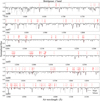 |
Fig. 2 Same as Fig. 1 but for the J band (echelle orders 48–43). |
| In the text | |
|
Fig. 3 log τRoss of the line-forming layers of the lines preselected in Sect. 3.3 as functions of the EP, the X index at 3850 K, the model depth dOnlyOne , the model EW, and the reduced model EW. Top and bottom panels show the results with employed line lists of VALD3 and MB99, respectively. The vertical error bar represents the range of Rosseland-mean optical depth where the contribution function for the line is larger than the half of the maximum value at log τRoss. Horizontal black dashed line at log τRoss = −3.0 indicates the final criteria of our line selection. |
| In the text | |
|
Fig. 4 Examples of how [Fe/H] is determined from each absorption line as a function of vmicro : here for the case for Betelgeuse. Top and bottom panels show the results with VALD3 and MB99, respectively. Left panels show the measurements for all the Fe I lines preselected in Sect. 3.3, and middle panels do for the lines satisfying conditions (i)–(v) in the main text (Sect. 3.5.2) and eventually used. Right panels show the measurements after the correction term Δ[Fe/H]i defined in Eq. (8) subtracted. Each curve in the figures corresponds to each absorption line color-coded according to log τRoss of the line-forming layer of the line; a lighter color corresponds to a larger log τRoss and thus a smaller EW. The dot on each curve indicates the [Fe/H] value determined with the corresponding vmicro . No dots are plotted where the fitting for a line with a value of vmicro failed. |
| In the text | |
|
Fig. 5 Correction term to the determined [Fe/H] values for each line for VALD3 as functions of EP (top-left panel), X index at 3850 K (top-middle), log τRoss (top-right), and wavelength in the standard air (bottom). Black dots show |
| In the text | |
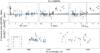 |
Fig. 6 Same as Fig. 5 but for MB99. |
| In the text | |
|
Fig. 7 Error budget of [X/H] measurements. Left panels show the medians of the absolute values of the three sources of errors (∆b , |
| In the text | |
|
Fig. 8 Comparison of our results and those of Levesque et al. (2005) for the RSGs included in both samples: Teff and log 𝑔. |
| In the text | |
|
Fig. 9 Comparison of our results and those of Luck & Bond (1989) for the RSGs included in both samples: stellar parameters and [Fe/H]. Top panels show Teff and log g, which are used in common with VALD3 and MB99. Middle and bottom panels show vmicro and [Fe/H] determined with VALD3 and MB99, respectively. |
| In the text | |
|
Fig. 10 Relation between log g and vmicro . Red closed circles and magenta closed squares indicate the values that we determined for the target RSGs with VALD3 and MB99, respectively. Orange open circles indicate the values for the five solar-metallicity red giants among the Gaia FGK benchmark stars (Heiter et al. 2015) used in T21. Blue solid lines show the relation used in the ASPCAP code for APOGEE DR13 (Holtzman et al. 2018) for the log g ranges of their calibrating sample, with the extrapolated relation indicated by blue dotted lines. Green and pink dashed lines indicate the relations calibrated by Adibekyan et al. (2012) and Dutra-Ferreira et al. (2016), respectively, for Teff = 3500 and 4000 K, with the log g ranges of their calibrating samples indicated by shades in the respective colors. |
| In the text | |
|
Fig. 11 Metallicities of RSGs compared with the radial metallicity gradient of Cepheids for the Galactocentric distance (RGC). Filled red circles (top panel) and filled magenta squares (bottom panel) show the derived [Fe/H] of our target RSGs for VALD3 and MB99, respectively. Blue dots show [Fe/H] of Cepheids (Luck 2018) within 5 < R < 14 kpc as an indicator of the radial metallicity gradient of young stars. Blue dashed lines show the linear fit to the Cepheids’s metallicities. Open brown symbols show the weighted-mean metallicities and their corresponding standard errors of RSGs in star clusters or star-forming complexes within 6 ≲ RGC ≲ 10 kpc measured by some previous works: Gazak et al. (2014) depicted with a diamond, Alonso-Santiago et al. (2017, 2018, 2019, 2020) and Negueruela et al. (2021) with triangles, and Fanelli et al. (2022) with a pentagon. |
| In the text | |
|
Fig. 12 Box plot of vmicro determined in this work (marked as TW) and previous works for RSGs plotted in Fig. 11: Gazak et al. (2014) as G14, Alonso-Santiago et al. (2017, 2018, 2019, 2020) as A17–A20, respectively, Negueruela et al. (2021) as N21, and Fanelli et al. (2022) marked as F22. |
| In the text | |
|
Fig. 13 Chemical abundances of RSGs after subtracting the radial abundance gradients of Cepheids. Filled red circles and filled magenta squares show the weighted mean and standard error of the derived [X/Fe] of our targets RSGs for VALD3 and MB99, respectively, after subtracting the radial abundance gradients of Cepheids, which are tabulated in Table D.2 as Mean. Open symbols show those for RSGs by the works measuring [X/Fe] as well as [Fe/H] among those cited in Fig. 11: Alonso-Santiago et al. (2017, 2018, 2019, 2020) with green, brown, pink, and cyan/blue triangles, respectively, and Fanelli et al. (2022) with yellow pentagons. We note that we show the results for all the elements for which we determined the abundances of RSGs, except for [K/Fe], as the abundance for Cepheids were not measured by Luck (2018). |
| In the text | |
|
Fig. C.1 Ratio of partial pressures p of some of major molecules and atoms to the total gas pressure pall: CN in red, CO in purple, N2 in brown, TiO in pink, C I in blue, N I in orange, O I in green, and Fe I in gray. The results here were calculated using MOOG for the set of stellar parameters of RSG3 (see Sect. 3.3). |
| In the text | |
Current usage metrics show cumulative count of Article Views (full-text article views including HTML views, PDF and ePub downloads, according to the available data) and Abstracts Views on Vision4Press platform.
Data correspond to usage on the plateform after 2015. The current usage metrics is available 48-96 hours after online publication and is updated daily on week days.
Initial download of the metrics may take a while.