| Issue |
A&A
Volume 693, January 2025
|
|
|---|---|---|
| Article Number | A182 | |
| Number of page(s) | 14 | |
| Section | Cosmology (including clusters of galaxies) | |
| DOI | https://doi.org/10.1051/0004-6361/202452285 | |
| Published online | 15 January 2025 | |
Testing the thermal Sunyaev-Zel’dovich power spectrum of a halo model using hydrodynamical simulations
1
Institut d’Astrophysique de Paris, UMR 7095, CNRS & Sorbonne Université, 98 bis Boulevard Arago, F-75014 Paris, France
2
Department of Astronomy and Steward Observatory, University of Arizona, 933 North Cherry Avenue, Tucson, AZ 85721, USA
3
Department of Physics, University of Arizona, 1118 E. Fourth Street, Tucson, AZ 85721, USA
⋆ Corresponding author; This email address is being protected from spambots. You need JavaScript enabled to view it.
Received:
17
September
2024
Accepted:
28
November
2024
Abstract
Statistical properties of large-scale cosmological structures serve as powerful tools for constraining the cosmological properties of our Universe. Tracing the gas pressure, the thermal Sunyaev-Zel’dovich (tSZ) effect is a biased probe of mass distribution and, hence, can be used to test the physics of feedback or cosmological models. Therefore, it is crucial to develop robust modelling of hot gas pressure for applications to tSZ surveys. Since gas collapses into bound structures, it is expected that most of the tSZ signal is within halos produced by cosmic accretion shocks. Hence, simple empirical halo models can be used to predict the tSZ power spectra. In this study, we employed the HMx halo model to compare the tSZ power spectra with those of several hydrodynamical simulations: the Horizon suite and the Magneticum simulation. We examine various contributions to the tSZ power spectrum across different redshifts, including the one- and two-halo term decomposition, the amount of bound gas, the importance of different masses, and the electron pressure profiles. Our comparison of the tSZ power spectrum reveals discrepancies between the halo model and cosmological simulations that increase with redshift. We find a 20% to 50% difference between the measured and predicted tSZ angular power spectrum over the multipole range ℓ = 103 − 104. Our analysis reveals that these differences are driven by the excess of power in the predicted two-halo term at low k and in the one-halo term at high k. At higher redshifts (z ∼ 3), simulations indicate that more power comes from outside the virial radius than from inside, suggesting a limitation in the applicability of the halo model. We also observe differences in the pressure profiles, despite the fair level of agreement on the tSZ power spectrum at low redshift with the default calibration of the halo model. In conclusion, our study suggests that the properties of the halo model need to be carefully controlled against real or mock data to be proven useful for cosmological purposes.
Key words: methods: numerical / galaxies: clusters: general / large-scale structure of Universe
© The Authors 2025
 Open Access article, published by EDP Sciences, under the terms of the Creative Commons Attribution License (https://creativecommons.org/licenses/by/4.0), which permits unrestricted use, distribution, and reproduction in any medium, provided the original work is properly cited.
This article is published in open access under the Subscribe to Open model. This email address is being protected from spambots. You need JavaScript enabled to view it. to support open access publication.
1. Introduction
The thermal Sunyaev-Zel’dovich (tSZ) effect (Sunyaev & Zeldovich 1970) arises when cosmic microwave background (CMB) photons are inverse Compton scattered by hot electrons, which leads to an energy shift of the CMB photons. The tSZ effect thus manifests as a distortion of the CMB black-body spectrum. By measuring this distortion, it is possible to infer astrophysical properties of the hot gas in galaxy clusters, and, in particular, their pressure on which the tSZ signals scale, as well as cosmological information.
It is possible to observe this effect on wide fields to create tSZ maps with Planck (Planck Collaboration XXII 2016) and the South Pole Telescope (SPT) (Bleem et al. 2022), for example, or on individual galaxy clusters, as done by Planck (Planck Collaboration XXIX 2014), Atacama Cosmology Telescope (ACT) (Menanteau et al. 2010), and SPT (Plagge et al. 2010) for example and will be studied with the New IRAM Kids Arrays (NIKA2) ground-based telescope (Perotto et al. 2023). As tSZ data become better resolved (with reduced levels of noise and systematics), it is important to have a robust modelisation because it is a foreground for the CMB but also a probe of the distribution of the baryonic matter which can help us to obtain better astrophysical and cosmological constraints. On the cosmological side, the amplitude of the tSZ is extremely sensitive to σ8 (e.g. Komatsu & Kitayama 1999; Refregier et al. 2000; Seljak et al. 2001; Komatsu & Seljak 2002; McCarthy et al. 2014; Bolliet et al. 2018). It can also be used to study early dark energy model (e.g. Sadeh et al. 2007; Waizmann & Bartelmann 2009). On the other hand, the tSZ is sensitive to astrophysics phenomena such as active galactic nuclei (AGN) feedback that redistributes mass and modifies the pressure of the hot plasma in massive halos (e.g. McCarthy et al. 2014, 2023; Le Brun et al. 2015; Spacek et al. 2018; Lee et al. 2022; Moser et al. 2022; Pandey et al. 2023).
To be able to extract even more information, the tSZ has been used in correlation with other probes. Many combined cross-correlation analyses have been performed, for example, the correlation between the tSZ signal and the weak lensing signal has been widely used to constrain cosmological parameters and nuisance parameters (e.g. Van Waerbeke et al. 2014; Ma et al. 2015; Osato et al. 2020; Tröster et al. 2022). More recently, Fang et al. (2024) developed a joint halo model to correlate tSZ, weak lensing, CMB lensing, and galaxy density (in total ten different two-point functions) to obtain even tighter constraints jointly on cosmological parameters and astrophysical parameters. Incorporating the tSZ probe is beneficial due to its sensitivity to baryonic physics. From this paper, one can note that, by including cross-correlations with additional tracers, the figure-of-merit can be improved by a factor of two and reduced notably the fraction of sky needed. By adding stronger priors on the halo model, in particular on the parameters required to model the tSZ pressure profile, one can gain even more on the figure-of-merit, which emphasizes the need for more robust tSZ models.
Originally, the tSZ power spectrum was modelled through the Press-Schechter formalism (e.g. Komatsu & Kitayama 1999; Refregier et al. 2000; Seljak et al. 2001). First studies with this formalism only account for correlation within clusters (known as the one-halo term) and Komatsu & Kitayama (1999) added for the first time the contribution of the correlation among clusters (known as the two-halo term). To improve the prediction, the Press-Schechter formalism is replaced by a halo model that depends mostly on the distribution of halos, halo bias, and electron pressure profile. Refregier & Teyssier (2002) made the first comparison between the tSZ power spectrum obtained with such a model and measurement in simulation. Once the limitations of the simulation were taken into account, the prediction from the halo model was in good agreement with the simulation. Many works continue to model the tSZ power spectrum with different parametric choices in a halo model framework to improve the agreement of the model with improved simulations and measurement. For cosmological analysis, one of the most used halo model is HMx, developed by Mead et al. (2020) (e.g. in Tröster et al. 2022). It is also possible to study the tSZ with non-parametric modelisation with machine learning techniques as done with the camels simulations (Moser et al. 2022) or with the the three hundred project (Ferragamo et al. 2023) for example.
For this work, we focused on and used the HMx halo model developed by Mead et al. (2020). This halo model was calibrated on the BAHAMAS simulation (McCarthy et al. 2017, see a small description of the simulation in Sect. 3.5 of this paper) at the level of the response power spectrum, and we used the model calibrated for the matter-pressure power spectrum. We explored how the predictions and components of this model compare with the Horizon suite (Dubois et al. 2014, 2016) and the Magneticum (Dolag et al. 2016) simulation. This study allowed us to extract the tSZ signal of the simulations to gauge the uncertainties associated with subgrid modelling. We also explored the importance of different mass bins and redshift ranges, to understand better where the modelisation needs to be improved, in particular for the correlation between CMB lensing and tSZ signal of clusters.
This paper is organised as follows: in Sect. 2 we describe the HMx halo model. We continue with a description of the Horizon suite and Magneticum simulation in Sect. 3. In Sect. 4 we present the results of the comparison of the power spectrum and angular power spectrum. In Sect. 5 we discuss the different properties that can impact the difference between prediction and measurement. Finally, we draw our conclusions in Sect. 6.
2. Halo model framework
We recall in the following the main assumptions and properties of a classical halo model and then describe the specifics of HMx.
2.1. Halo model
A halo model assumes that all matter in the universe is partitioned into spherical and symmetrical halos of different masses and sizes. Depending on the scale of interest, the statistical properties of the matter distribution will depend on the overall distribution of halos in the universe (large scale) or on the distribution of matter within a given halo, integrated over the distribution of halo sizes and masses (small scale). Such a model relies on a limited number of components, including the properties of the matter distribution at large scales in the linear regime (given by the cosmological model), the distribution of halo mass (or halo mass function) n(M), the halo bias b(M), and the halo profile. These components must be modelled and can be calibrated using simulations or data. Starting from this main idea, it is possible to extend this formalism to other tracers of large-scale structures, provided that the halo properties as seen by those tracers and their correlations with the matter distribution are known.
In this context, the power spectra of the different tracers of the large-scale structure (LSS) are often separated into their one-halo (probing the intra-halo statistical properties of the tracer, typically at small scales) and two-halo parts (probing the distribution of halos, often at large scales) Puv(k) = P1H, uv(k)+P2H, uv(k), where u and v are two three-dimensional (3D) fields.
In detail, the one- and two-halo power spectrum of a given tracer of the LSS follow
 (1)
(1)
![Mathematical equation: $$ \begin{aligned} P_{\mathrm{2H},uv}(k)&= P_{\rm lin}(k)\prod _{i=u}^{v}\left[\int _0^\infty b(M)W_i(M,k)n(M)\mathrm{d}M\right], \end{aligned} $$](/articles/aa/full_html/2025/01/aa52285-24/aa52285-24-eq2.gif) (2)
(2)
where Plin is the linear matter power spectrum and the Fourier transform of the field u is
 (3)
(3)
with  the averaged radial profile for the field u, function of mass M and comoving radius
  .
.
While the matter, pressure, and matter-pressure 3D power spectra can be measured in simulations and are required to compute the correlation of tSZ with other LSS tracers, they are usually not directly observable. What can be measured easily in microwave sky maps are angular power spectra Cuv(ℓ) which are projected along the line of sight. From the 3D power spectra, one can compute the angular power spectrum Cuv(ℓ)
 (4)
(4)
where ℓ is the multipole moment,  the Hubble radius,
  the comoving angular-diameter distance (for a flat universe we thus have
  ),
),  is the redshift at comoving distance
  , and
, and  . For the Compton-y parameter, the projection kernel Xy is:
 (5)
(5)
where a is the expansion factor, σT is the Thompson scattering cross-section, me is the electron mass, and c is the speed of light.
2.2. HMx parametrisation
We recall in the following the details of one of the main approaches used to approximate the power spectrum of different tracers of large-scale structures: the HMx model (Mead et al. 2020). This semi-analytical model was built upon the classical halo model and included additional degrees of freedom that were fit to a suite of hydrodynamical simulations (the BAHAMAS simulation McCarthy et al. 2017). The HMx model predicts the (cross-) power spectra of different tracers, including tSZ, within a single framework and includes physics-inspired parameters that are common to some of the different tracers. This approach is particularly useful when analysing a large number of tracers simultaneously in the context of cosmological surveys, as we demonstrate in Fang et al. (2024).
Different halo models for different observables and assuming different hypotheses have been developed over the years (e.g. Maniyar et al. 2021; Bolliet et al. 2023). Each of them proposes different modelling for the components described above and different ways to calibrate the parameters of those models. The HMx (Mead et al. 2020) variant of these models is one of the most widely used for cosmological data analysis (e.g. for weak lensing analysis such as in Tröster et al. 2022). It further features several interesting features that make it particularly suitable as a base for comparison with simulations, as we will do here. HMx already implements several probes of the LSS which makes it particularly useful in the context of probes cross-correlations. Its implementation is also very modular, allowing for relatively easy modifications of the different model components, as well as change in ranges of integration, a feature that will be key to our comparisons, as we will discuss below. Finally, a specificity of this model is that all the parameters of the different approximations used to describe the halo properties are fitted simultaneously against the BAHAMAS simulation power spectra (see the end of this subsection or in Mead et al. 2020, for more details). This is a different approach from one where each component and parameter of the model are fitted separately against data or simulations (for example, fitting the parameters of the halo profile against stacked halo profiles measured in simulations). This simultaneous fitting ensures the fidelity of the power spectra prediction, but it may come at the expense of the physical meaning of the parameters and their values. This can be an issue if one wants to improve the model by obtaining stronger and physically inspired priors on those parameters from data or simulations. For all of those reasons, we decided to retain HMx as our reference halo model in this work.
The mass function n(M) adopted in HMx is the one from Sheth & Tormen (1999). The halo bias function was then derived from this mass function using the peak-background split formalism (Mo & White 1996; Sheth et al. 2001). In the case of tSZ, the field u is the electron pressure, defined as
 (6)
(6)
where mp is the proton mass, μe is the mean gas-particle mass per electron divided by the proton mass, kB is the Boltzmann constant, and ρbnd is the halo bound gas density and represents the gas which is inside the proper virial radius rv, defined as
![Mathematical equation: $$ \begin{aligned} \rho _{\rm bnd} \propto \left[\frac{\ln (1+r/r_{\rm s})}{r/r_{\rm s}}\right]^{1/(\Gamma -1)}, \end{aligned} $$](/articles/aa/full_html/2025/01/aa52285-24/aa52285-24-eq15.gif) (7)
(7)
where Γ is the polytropic index for the gas, and rs is the halo scale radius parameter, specified via the concentration relation cM = rv/rs
The virial mass Mv was defined as where the total mean matter density in the halo within the (proper) virial radius rv is Δv (the virial-collapse density contrast) times the critical density:
 (8)
(8)
where ρc(z) = 3H(z)2/(8πG) is the critical density of the Universe at redshift z, G is the gravitational constant, H(z) is the Hubble expansion factor, and where Δv comes from the ΛCDM fitting function of Bryan & Norman (1998). This was the same definition of virial mass as in Mead et al. (2020), but we caution that their masses were measured in dark matter-only simulation whereas we used the one of the hydrodynamical simulations directly.
The gas ejected outside the virial radius by feedback processes did not contribute to the one-halo term. The formalism assumed that the gas was associated with the initial density of the associated halo but can now be far from it. It was however taken into account by adding it back to the two-halo term only, following the treatment done by Fedeli (2014) and Debackere et al. (2020). For more details about the treatment of the ejected gas, we refer the reader to Mead et al. (2020). The model further assumed that all the gas is ionized, and for the bound gas, the Komatsu & Seljak (2001) profile was used to determine the gas temperature Tg:
 (9)
(9)
which assumes hydrostatic equilibrium. The virial temperature Tv was defined as:
 (10)
(10)
where μp is the mean gas-particle mass divided by the proton mass, α encapsulates deviations from a virial relation and thus acts as a hydrostatic bias (here we have α = 0.8471).
Such model particularly enhances the contribution of high-mass halos to the tSZ power spectrum, while low-mass halos are deficient in gas. Moreover, the amplitude of the one- and two-halo terms are more sensitive to high-mass halos, as the Fourier transform of the pressure profile Wp(M, k → 0) is proportional to M5/3. In comparison, the Fourier transform of the matter field Wm(M, k → 0) scales as M. This can be explained by the fact that the electron pressure follows the gas density but emanates only from the highest gas-density peaks because the temperature is higher, thus boosting the electron pressure.
For more details about the definition of the concentration relation, the fraction of bound gas, or other model’s components, we refer the reader to Mead et al. (2020). The default and best-fit values of the parameters of the model, that were fitted against the BAHAMAS simulations (McCarthy et al. 2017), can be found in Tables 1 and 2 of Mead et al. (2020), respectively.
In detail, the fits were performed on the BAHAMAS simulation 3D power spectrum response between z = 0 and 1 and for k between 0.015 and 7 h−1 Mpc for stars, matter, matter & electron pressure, or matter, cold dark matter (CDM), gas & stars jointly. The fits covered four different cosmological models. In the case of tSZ, the parameters were fitted on the matter-electron pressure cross-power spectrum only and used as is for the predictions of the electron pressure auto-spectrum. The Mead et al. (2020) paper argues that this approach provides the lowest error on the pressure auto-power spectrum as the pressure auto-power spectrum is difficult to fit because of its high Poisson noise. The relative difference between the BAHAMAS simulation and prediction, averaged linearly over z between 0 and 1 and logarithmically over k between 0.015 and 7 h Mpc−1, is of 2% for the matter auto-power spectrum, 15% for the matter-pressure, 25% for the pressure auto-power spectrum. As can be seen, the prediction has a relatively low fidelity for the pressure auto-spectrum. Several reasons can explain this fact. The halo model makes several strong hypotheses, such as halos trace the underlying linear matter distribution with a linear halo bias, halo profiles are perfectly spherical with no substructure and no scatter at fixed mass, and there is nothing to prevent halos from overlapping. While these hypotheses provide a reasonable approximation of the physics at play in the case of the matter distribution, explaining the good precision in the case of the matter power spectrum and fair in the case of the cross-spectrum, they are not necessarily correct for the electron pressure distribution. Furthermore, the tSZ sensitivity to high-mass clusters also limits the predictive power for different reasons. First, because of the limited size of the simulations, calibration for high-mass clusters can be imperfect. Second, the mass scaling parametrisation must extrapolate from halo masses probed by the matter-pressure power spectrum to those probed by the pressure auto-power spectrum, which involves highest masses.
The relatively low fidelity of the model for the electron pressure auto-spectrum, the fact that the parameters lose some of their physical meaning since they were fitted to reproduce the simulation power spectra and the risk of over-fitting the model to a particular simulation and its limitations are all excellent arguments to revisit the HMx predictions and compare them with other simulation suites. In this work, we used the Horizon and Magneticum simulations. Similar to the approach taken by Mead et al. (2020), we also focused on the matter-pressure cross-spectra, which is the best predicted observable of HMx model we are using.
2.3. Angular power spectrum prediction
In the rest of this article, we compared the model predictions with measurements in the simulations. However, it is not useful to discuss differences occurring at redshifts that do not contribute significantly to the angular power spectra. For example, Komatsu & Seljak (2002) showed that the contribution of clusters at z > 10 is negligible to the pressure angular power spectrum. We used the predictions from HMx to address this question. The pressure angular power spectrum obtained using different redshift ranges of integration is shown on the left panel of Fig. 1, where we look at the angular power spectrum when integrating up to different redshifts. We can note that integration up to z = 3 or z = 4 captures more than 97% of the power for ℓ between 10 and 104. Limiting ourselves to z = 2 will only lead to a dramatic loss of ∼17% of validity after ℓ = 4 × 10³. We have also looked at the contribution coming from the one-halo term when integrating up to a given z for different ℓ. Except when z is sufficiently small and ℓ large, corresponding to the interior of halos, more than 90% of the angular power spectrum comes from the one-halo term. This behaviour can be due to the change of slope in the pressure profiles of halos, or to the fact that the contrast of pressure is smaller on the inner part of halos. These two conclusions imply that the modelisation of the electron pressure profiles up to z = 4 will impact our results and need to be well understood.
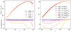 |
Fig. 1. Predicted pressure angular power spectrum when integrating up to different redshifts in different colours (on the left) or between z = 0.02 and z = 10 for different maximal mass in different colours (on the right) as a function of the angular scale ℓ. |
In the previous section, we noted that the power spectra are dominated by high-mass clusters. However, depending on the simulation characteristics, the number of such high-mass objects in our simulations will be limited, which we need to take into account when comparing the model predictions with the simulations. As a first step in investigating the impact of high-mass objects, we show in the right panel of Fig. 1 the contribution of the different halo masses to the power spectra, as we vary the maximum mass considered in HMx (see also, e.g. Refregier et al. 2000; Battaglia et al. 2012). Our reference here is the default maximum mass used in HMx: Mmax = 1017 h−1 M⊙. We can note that the different ℓ are not affected in the same way; this choice of maximal mass impacts the most the values of ℓ = 50 − 60. We can see that integrating up to Mmax = 1016 h−1 M⊙ makes almost no differences. Using Gumbel statistics, Davis et al. (2011) found that it is very unlikely to have dark matter halos with M > 1016 h−1 M⊙ within a volume of 1 h−1 Gpc, we can extrapolate that it is also the case within the observable Universe. The prediction still changes a bit because the halo mass function predicts that it is possible to have such halos, but for analysis with real data, we will probably never use this maximal mass (Holz & Perlmutter 2012). If we are integrating up to Mmax = 2 × 10¹⁵ h−1 M⊙ instead of Mmax = 4 × 10¹⁵ h−1 M⊙ we loose maximum 20% of the signal instead of a few percent. This implies that the masses of a few 1015 h−1 M⊙ must be well-modelled in our prescription.
3. Simulations
To pursue this analysis, we are interested in the comparison of the HMx prediction with measurement in different simulations. We thus used four simulations: Horizon-AGN, Horizon-noAGN, Horizon-Large, and Magneticum and we recall their main characteristics in this section. This allowed us to compare prediction and measurement with simulations containing different physics and implementation schemes but also to analyse for the first time the tSZ signal in the Horizon simulations. We also recall the main characteristics of the BAHAMAS simulation because they are the ones used to calibrate HMx, but we are not analysing them within this paper.
3.1. Horizon-AGN
The Horizon-AGN simulation (Dubois et al. 2014) is a cosmological hydrodynamical simulation of 100 h−1 Mpc comoving volume, with 10243 dark matter particles, leading to a resolution of MDM, res = 8.3 × 10⁷ M⊙. The simulation uses the adaptive mesh refinement code RAMSES (Teyssier 2002) that can refine up to a minimum cell size of Δx ≃ 1 kpc (comoving). The cosmology is a standard ΛCDM cosmology compatible with WMAP-7 (Komatsu et al. 2011) with {Ωm, ΩΛ, σ8, Ωb, ns}={0.272, 0.728, 0.81, 0.045, 0.967} and H0 = 70.4 km s−1 Mpc−1. Multiple redshifts between z = 0.018 and z = 38.3 are available, allowing us to perform redshift space analysis. In the following, we focus our study on redshifts between 0 and 5. More details about the physics and refinement scheme are available in Dubois et al. (2014), but we summarise here the main aspects. The simulation includes gas cooling (Sutherland & Dopita 1993), and a uniform UV background (Haardt & Madau 1996) with redshift of reionisation zr = 10. It follows star formation using a Schmidt law with 2% star formation efficiency and the associated feedback from stellar winds, type II and type Ia supernovae (Dubois & Teyssier 2008), as well as feedback from active galactic nuclei (AGN) powered by Bondi-Hoyle-Lyttleton accretion limited at Eddington with jet/radio or heating/quasar mode depending on the accretion rate relative to Eddington (Dubois et al. 2012).
3.2. Horizon-noAGN
The Horizon-noAGN simulation (Dubois et al. 2016) has the same initial conditions, sub-grid modelling, and cosmology as the Horizon-AGN simulation, only the physics is different. This simulation contains no black hole formation and therefore no AGN feedback. This leads to a significant overshoot of the baryonic mass content in galaxy groups and clusters, and in particular of their gas fraction, at the high-mass end (Beckmann et al. 2017; Chisari et al. 2018).
3.3. Magneticum
The Magneticum suite of simulations (Dolag et al. 2016) are cosmological hydrodynamical simulations with different box sizes and cosmologies. In this work we use the medium resolution Box1a simulation of 896 h−1 Mpc comoving volume, with 15123 dark matter and (initial) gas particle masses of 1.3 × 10¹⁰ h−1 M⊙ and 2.6 × 10⁹ h−1 M⊙, respectively. For analysing the properties of lower mass halos (see Section 5.2), we use Box2 which has a smaller volume of 352 h−1 Mpc comoving volume but a better mass resolution of 6.9 × 10⁸ h−1 M⊙ and 1.4 × 10⁸ h−1 M⊙ for dark matter and gas particles respectively. The simulations use the smooth particle hydrodynamics (SPH) code P-GADGET3 (Springel et al. 2005). The boxes that we are using also follow a WMAP-7 cosmology (Komatsu et al. 2011) with {Ωm, Ωb, σ8, h, ns}={0.272, 0.0456, 0.809, 0.704, 0.963}. We also have access to the redshifts between 0 and 5. We summarise here the main physical aspects. The simulation includes gas cooling, star formation, and winds (Springel & Hernquist 2003). The metals, stellar population, and chemical enrichment, SN-Ia, SN-II, AGB follow Tornatore et al. (2003, 2006) with the new cooling tables of Wiersma et al. (2009). There are also black holes and AGN feedback (Hirschmann et al. 2014).
3.4. Horizon-Large
We ran the Horizon-Large simulation specially for this work to improve the comparison between the Horizon and Magneticum suite of simulations. This particular simulation is a cosmological hydrodynamical simulation of 896 h−1 Mpc comoving volume (a similar box size than that of the Magneticum simulation described in the previous subsection), with 10243 dark matter particles, leading to a resolution of MDM, res = 6 × 10¹⁰ M⊙. The simulation uses the RAMSES (Teyssier 2002) code and the grid is allowed to refine up to a spatial resolution of 10 kpc (comoving). The cosmology is the same as that of the Horizon-AGN and Horizon-noAGN simulations. The physics is simpler than the other simulations: it only contains gas cooling and UV background heating below zr and no galactic physics (no star formation nor feedback) for computational reasons. It is a reasonable approximation to large-scale boxes with more complex subgrid physics (such as, e.g. Magneticum) as the most massive clusters that are captured in such big volumes – and which dominate the tSZ signal (see Section 2.2) – are the most insensitive to mass redistribution due to feedback (e.g. Gonzalez et al. 2013; Le Brun et al. 2014; McCarthy et al. 2018; Chisari et al. 2018). This simulation is also used to probe the cosmic variance with a similar numerical treatment of the hydrodynamics than in the other Horizon simulations.
3.5. BAHAMAS
The BAHAMAS simulations are a suite of hydrodynamical simulations of 400 h−1 Mpc with the WMAP 9-yr (Hinshaw et al. 2013) and Planck 2013 (Planck Collaboration XVI 2014) cosmology. The simulations contain 2 × 10243 particles leading to a resolution of Mbaryon, res = 3.85 × 10⁹ h−1 M⊙ (Mbaryon, res = 4.45 × 10⁹ h−1 M⊙) and MDM, res = 7.66 × 10⁸ h−1 M⊙ (MDM, res = 8.12 × 10⁸ h−1 M⊙), respectively for a WMAP-9 (Planck) cosmology. The hydrodynamic code and subgrid physics are the same as the ones in the OWLS (Schaye et al. 2010) and cosmo-OWLS (Le Brun et al. 2014; McCarthy et al. 2014) projects. The simulations include radiative cooling and heating, with a reionization that occurs at zr = 9, a star formation rate, and stellar evolution and chemical enrichment. It also contains a black hole and AGN feedback with three strengths of AGN feedback, from the smaller to the bigger: 107.6 K, 107.8 K, and 108.0 K. More details about the physics are available in Schaye et al. (2010).
3.6. Mass cut to compare different simulations
Because the simulations have different box sizes and physics, the halo mass function can differ and, as seen on the right of Fig. 1 and related text, the maximum mass chosen for the HMx prediction will impact our results. In Fig. 2, we present the halo mass function of the four simulations we are working with (Horizon-AGN, Horizon-noAGN, Horizon-Large, and Magneticum) compared with the theoretical halo mass function from Sheth & Tormen (1999), which is the one used in HMx. This analytical mass function has been fitted on dark matter halos. For the Horizon simulations, the halos were identified with the adaptaHOP halo finder (Aubert et al. 2004), and we only kept the halos (and subhalos) with at least 100 particles. For Magneticum, the halos were identified with a standard Friends-of-Friends algorithm and subhalos with the subfind module (Springel et al. 2001; Dolag & Stasyszyn 2009). We see a relatively good agreement between the different simulations, nevertheless, they all have different maximal and minimal masses because of the difference in volume and mass resolution. We observe a lack of high-mass halos (except for the last bin of Horizon-AGN and Horizon-noAGN, which is probably just a binning effect), more important in the bigger simulations, and of low-mass halos in all the simulations. The trend observed at z = 0 is similar to the one at higher redshift. Since we are comparing an analytical function derived from dark matter-only halos with results from hydrodynamical simulations, discrepancies may be caused by the influence of baryons (cosmological accretion shocks, background UV heating, and feedback) on mass redistribution. The impact varies across different halo masses with fractional variations in good agreement with other studies (see, e.g. Vogelsberger et al. 2014; Sorini et al. 2025).
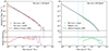 |
Fig. 2. Halo mass function at z = 0 for the Horizon-AGN, Horizon-noAGN, Horizon-Large, and Magneticum simulations in red, purple, green, and blue, respectively, with their associated Poisson noise as error bar. Each mass function is computed up to the maximal halo mass in the corresponding simulation. The analytical mass function from Sheth & Tormen (1999) is shown in black for comparison. Vertical lines indicate the minimum halo mass accessible in each simulation, defined as 100 times the dark matter mass resolution. The lower limits for Horizon-AGN and Horizon-noAGN are identical. |
We recall that we used the virial mass as the definition of our halo mass (defined in Eq. (8)). As mentioned in Sect. 2, the maximal mass chosen in HMx will significantly change the prediction on the pressure auto-power spectrum, it is thus important to take them into account when comparing the results from HMx and the one measured in the simulations. In the following of the paper, we used Mmax = 6.4 × 10¹⁴ h−1 M⊙ for Horizon-AGN and Horizon-noAGN simulations and Mmax = 2.6 × 10¹⁵ h−1 M⊙ for the Horizon-Large and Magneticum simulations. These two maximal masses are the maximum mass of Horizon-AGN and Magneticum, respectively. We have checked that the prediction using the maximal mass of Horizon-noAGN (or Horizon-Large) makes almost no difference, this is why we can compare the results of Horizon-noAGN with the prediction obtained for Horizon-AGN, and the results of Horizon-Large with the prediction obtained for Magneticum.
4. Results
In this section, we present our results on the comparison of the predicted (angular) power spectrum from HMx and the one measured in the different simulations. As some differences between the predictions and the measurements are expected (see Sect. 2), we now focus on characterizing the ones that matter the most for observations.
4.1. Power spectrum
The first straight-forward comparison concerns the pressure and matter-pressure power spectrum. We restricted our analysis to redshifts between 0 and ∼4, as higher redshifts do not significantly contribute to the angular power spectrum, as discussed in Sect. 2.3. We focused on quantifying differences of the tSZ signal from simulations that include different physical models than BAHAMAS (which HMx is calibrated on) and understanding how they propagate to higher redshifts.
To obtain the different power spectra from the simulations, we followed the procedure described in Appendix A. As a first check, we compared the matter auto-power spectrum of all the simulations at all redshift with the one predicted by HMx and we find a good agreement. The analysis reveals a ∼10% difference between the measurements and predictions, with no apparent trend in k or redshift. This test allows us to confirm our pipeline before moving to the analysis of pressure auto- or cross-power spectra.
4.1.1. Pressure auto-power spectrum
We first compare the pressure auto-power spectrum measured in the Horizon-AGN and Magneticum simulations to the one predicted by HMx as a function of redshift in Fig. 3. Additionally, the result of Horizon-noAGN and Horizon-Large at z ∼ 0 are included to emphasize the impact of different physics. We do not show their evolution with redshift since the trend is similar to the other simulations. At z ∼ 0, both Horizon-AGN and Horizon-noAGN predict an excess of power, even more important in Horizon-AGN. On the other hand, Horizon-Large shows a power deficit. Finally, Magneticum is in relatively good agreement with the prediction at every scale. We also observe that there is more power in the larger simulations, which is expected as they contain more massive halos (see also Sect. 2.3).
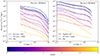 |
Fig. 3. Pressure auto-power spectrum as a function of redshift. The left panel shows the results for simulations with a box size of 100 h−1 Mpc, thus Horizon-AGN in dashed line compared to HMx in solid line, and Horizon-noAGN at z = 0 in dotted line. The right panel shows the results for simulations with a box size of 896 h−1 Mpc, thus Magneticum in dashed line compared to HMx in solid line, and Horizon-Large at z = 0 in dotted line. The power spectra go from z = 0 in dark blue to z = 4.25 in yellow. |
Then, we can examine the evolution with redshift. For all the simulations, we observe a relatively good agreement at low redshift with the predictions from HMx (up to z ∼ 1 for Horizon-AGN and Magneticum). However, as the redshift increases, discrepancies become more evident. We observed that the differences in the pressure power spectrum are not attributed to the one of the matter power spectra, suggesting that these discrepancies are more likely due to the modelling of the pressure rather than the matter. HMx predicts an excess of power at high redshift, indicating that the model’s physics fails to capture the nuances present in the simulations. We also notice that the measured power spectra are flatter than the predictions. Further investigations into these differences will be studied and discussed in Sect. 5.
4.1.2. Matter-pressure power spectrum
As we are using the HMx model calibrated on the matter-pressure power spectrum (see Sect. 2.2), we extended our analysis to examine the matter-pressure power spectrum to explore the agreement across different redshifts. Moreover, modelling the matter-pressure power spectrum is important for studying the correlation between weak lensing and pressure (that we are not doing here). In Fig. 4, we show the measurement obtained from the Horizon-AGN and Magneticum simulations compared to the HMx prediction as a function of redshift. Additionally, the result of Horizon-noAGN and Horizon-Large at z ∼ 0 are included to emphasize the impact of different physics. We do not show their evolution with redshift since the trend is similar to the other simulations. At z ∼ 0, as for the pressure auto-power spectrum, Horizon-AGN demonstrates an excess of power, Horizon-Large a lack of power, while Magneticum agrees well with the prediction. We now observe a good agreement between Horizon-noAGN and HMx.
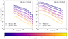 |
Fig. 4. Matter-pressure power spectrum as a function of redshift. The left panel shows the results for simulations with a box size of 100 h−1 Mpc, thus Horizon-AGN in dashed line compared to HMx in solid line, and Horizon-noAGN at z = 0 in dotted line. The right panel shows the results for simulations with a box size of 896 h−1 Mpc, thus Magneticum in dashed line compared to HMx in solid line, and Horizon-Large at z = 0 in dotted line. The power spectra go from z = 0 in dark blue to z = 4.25 in yellow. |
Then, we can examine the evolution with redshift. We observe a better agreement up to a comparable redshift (z ∼ 1.18 for both simulations) than for the pressure auto-power spectrum. This outcome is expected as HMx has been calibrated on the matter-pressure power spectrum up to z = 1. Moreover, the matter auto-power spectrum agrees well across all redshifts, mitigating the discrepancies in the pressure auto-power spectrum. At higher redshifts, the discrepancies caused by the pressure auto-power spectra persist.
Given the sensitivity of pressure to baryonic physics, such cross-correlations can serve as valuable tools for constraining astrophysical parameters (e.g. with the cosmic shear-tSZ cross-correlation with the flamingo simulations in McCarthy et al. 2023 or with the lensing-tSZ cross-correlation from KiDS-1000 (lensing), Planck and ACT (tSZ) in Tröster et al. 2022). Depending on the probes we are working with, it is crucial to adequately model different redshift ranges. With future surveys, we expect to be sensitive up to redshift two for probes such as the distribution of galaxies, tomographic studies, or weak lensing (e.g. with Euclid, Laureijs et al. 2011 or Roman, Eifler et al. 2024), our prediction thus needs to be trustable up to this redshift, which is qualitatively the case for the matter-pressure power spectrum.
4.2. Angular power spectrum
The observable accessed through surveys is the angular power spectrum, and its accurate prediction is crucial. Using the power spectra computed on the simulations or predicted by HMx, we used Eqs. (4) and (5) to obtain the pressure angular power spectrum. We integrated these spectra over the redshift range z = 0.02 to z = 4 (according to the discussion in Sect. 2.3) and we limited our analysis to the Nyquist frequency: kNy ∼ 16 h−1 Mpc for Horizon-AGN and Horizon-noAGN, while going up to kNy ∼ 3.6 h−1 Mpc for Magneticum and Horizon-Large (using a projection on 10243 to achieve a comparable kNy to that of Magneticum). At each redshift, the ℓ range accessible with the simulations varies, depending on the available k range (which is influenced by the size of the simulations). Choosing an ℓ range accessible to all the simulations across all redshifts between 0.02 and 4 would be quite narrow. To avoid this limitation and extract maximum information from the simulations, we opted for an interesting range of ℓ, filling the angular power spectrum with a zero for any inaccessible ℓ. We ensured to maintain the same behaviour in the angular power spectrum computed with the power spectrum of HMx, by cutting out at the same locations. We decided to compute the angular power spectrum for ℓ between 103 and 104 to encompass a range where the tSZ becomes an important foreground but remains accessible with future surveys. This pipeline limits our predictive power but allows us to infer the properties and behaviour of the different simulations and HMx.
The angular power spectra obtained from the different simulations are shown in Fig. 5 and compared with the HMx prediction. The agreement between Horizon-AGN and HMx improves at higher ℓ with differences reaching less than 10% between ℓ = 3 × 10³ and ℓ = 104. The power spectrum of Horizon-AGN (see Fig. 3), exhibits more power at low redshifts and less power at high redshifts compared to the prediction, and these discrepancies seem to compensate each other, resulting in a small difference in the angular power spectrum. In contrast, Magneticum shows an opposite trend, with better agreement at low ℓ where differences are less than 10% difference between ℓ = 103 and ℓ = 2 − 3 × 10³. For Horizon-noAGN and Horizon-Large, the general behaviour is quite similar, the simulations always have between 20% and 50% less power than HMx.
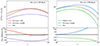 |
Fig. 5. Pressure angular power spectrum integrated between z = 0 and z = 4 for the different simulations in different colours and HMx in dark grey. The left panel shows the results for simulation with a box size of 100 h−1 Mpc, thus Horizon-AGN in red and Horizon-noAGN in purple. The right panel shows the results for simulation with a box size of 896 h−1 Mpc, thus Horizon-Large in green and Magneticum in blue. |
5. Discussion
In the previous section, we have emphasized the observed differences between prediction from HMx and measurement from the simulations (Horizon-AGN, Horizon-noAGN, Horizon-Large and Magneticum), in particular, the increased discrepancy when the redshift increases. In this section, we explore some effects that can partially explain the observed differences between prediction and measurement but also between the measurements in different simulations. It can give a hint at the intrinsic limitation of a halo model but also an avenue for improved prediction. We are thus exploring the consequences of using a halo model prescription in Sect. 5.1, the electron pressure profile in Sect. 5.2, and the differences between simulations in Sect. 5.3.
5.1. Halo model consequences
In this section, we are interested in studying the limitations caused by a halo model prescription. We explored the one- and two-halo decomposition, the validity of the bound gas assumption at different redshifts, and the importance of the different masses. This can help us understand the limitations that can bias or limit our predictive power.
5.1.1. One- and two-halo terms decomposition
To understand better the differences observed in the predicted and measured pressure auto-power spectrum (see Fig. 3 and related text), we explored the evolution of the one- and two-halo term contributions to the total power spectrum as a function of redshift. In Fig. 6, we show this decomposition for three different redshifts: z = 0.02, z = 1.16, and z = 3.01. For each redshift, we compared the Horizon-AGN power spectrum, the one predicted by HMx, and the one-halo and two-halo term predicted by HMx. As we increase the redshift, the contribution from the two-halo term becomes increasingly significant compared to the one-halo term at a given k. The increasing importance of the two-halo term is related to the scale at which the one- and two-halo terms intersect, which shifts towards higher k values. We observe that the excess of power in the HMx power spectrum at higher redshifts is thus dominated by the two-halo term at low k and by the one-halo term at high k. The excess of power in HMx suggests potential discrepancies in the distribution between the one- and two-halo terms, including the amplitude of each term at a given k scale as a function of redshift. At higher redshifts, there are only a few halos, the observable thus resembles the matter distribution, whereas at lower redshifts, more, and more massive, halos have formed. Thus, at low redshifts, the hypothesis that all the matter is within the halos is more accurate and the halos contribute more to the total power. Also, the contribution from the halos increases more rapidly than that from the diffuse gas. Finally, differences can suggest an inaccurate representation of the intergalactic medium effects by the two-halo term, in particular its amplitude.
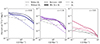 |
Fig. 6. Pressure auto-power spectrum as a function of redshift in the different panels. For every redshift, we show the power spectrum of Horizon-AGN in a coloured dashed line, the HMx prediction in a coloured full line, the predicted one-halo term in a coloured thin line, and the predicted two-halo term in a coloured dotted-dashed line. We superimpose the pressure auto-power spectrum within (without) one virial radius in a grey full line (grey dotted-dashed line). On the left, we show the result for z = 0.02, on the middle for z = 1.16, and on the right for z = 3.01. |
5.1.2. Validity of the bound gas assumption
The halo model contains some intrinsic limitations, as it assumes that all the matter is within spherical halos and that the one-halo term – which is the dominant contribution to the power spectra at low redshift (as shown by the coloured lines in Fig. 6 and discussed in the previous subsection) – only contains bound gas, which is gas inside the virial radius. To better understand the validity of this assumption, we investigated how the power spectrum differs when considering pressure inside or outside one virial radius of halos, compared to the prediction from HMx. These spectra are obtained by selectively masking gas pressure by masking either inside or outside one virial radius of halos. In Fig. 6, we show the contribution of bound and diffuse gas to the power spectrum measured from Horizon-AGN, and we find that the remaining simulations show similar trends. We compared the electron pressure auto-power spectra of Horizon-AGN to the one coming from inside (outside) one virial radius for three different redshifts: z = 0.02, z = 1.16, and z = 3.01. We observe that, at low redshift, most of the power comes from within one virial radius of halos. However, this assumption loses validity with increasing redshifts. Notably, at z = 3.01, there is more power coming from outside one virial radius of halos than inside. This implies the diminishing applicability of the halo model prescription at higher redshifts. Moreover, comparing the one-halo term to the power spectrum coming from inside one virial radius, reveals that at z = 0.02, the shape is consistent even if HMx lacks power. However, as redshift increases, discrepancies in shape emerge, contrary to the expectation that the one-halo term should be representative of the power spectrum within one virial radius of the halos. These observations can partially explain the discrepancies observed in Fig. 3 with increasing redshift. Given these limitations, it becomes imperative to consider them when evaluating the cross-correlation with other probes.
5.1.3. Importance of the halo mass
To go one step further in our test of the halo model, we investigated the contribution of each mass bin to the overall power spectrum. We performed this study for the different simulations (Horizon-AGN, Horizon-noAGN, Horizon-Large and Magneticum), and redshifts, and they all show a similar trend, thus, we are only presenting and quantify the results for Horizon-AGN at z = 0.02 in Fig. 7. We compared the electron pressure auto-power spectra with the one coming from inside one virial radius of the halos in different mass bins at z = 0.02. We can clearly see that most of the power emanates from the highest mass bin, despite its relatively low population (for Horizon-AGN, the highest mass bin contains only 0.006% of the total number of halos). The lower the mass bin, the lesser its contribution to the total power spectrum. A reduction of approximately one order of magnitude is observed with each logarithmic decrease in mass bin. This shows the importance of ensuring that the halo model, particularly the electron pressure profile, accurately reflects the characteristics of the highest mass halos, in agreement with the conclusion done in Sect. 2.3. However, given that the higher mass halos are less common occurrences, it may be worth masking them to mitigate the connected non-Gaussian covariance and tighten cosmological or astrophysical constraints, as explored in Osato & Takada (2021).
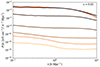 |
Fig. 7. Pressure auto-power spectrum of the total Horizon-AGN simulation in red compared to the signal coming from within one virial radius of different mass bin. The highest mass bin is in dark brown and corresponds to the mass bin 14 < log(Mv/M⊙ h−1) < 15, we then decrease of one dex for every curve until reaching the lowest mass bin in yellow, which corresponds to the mass bin log(Mv/M⊙ h−1) < 10. |
5.2. Halo pressure profiles
One of the main components of the model is the electron pressure profile, defined in Eq. (6). This profile not only represents a major aspect of the model but also constitutes the primary component of the one-halo term. As demonstrated in Fig. 6, the one-halo term is the predominant contribution to the power spectrum at low redshifts, further influencing the angular power spectrum. Consequently, in Fig. 8 we present the electron pressure profile measured in the different simulations (Horizon-AGN, Horizon-noAGN, Horizon-Large, and Magneticum) compared to the prediction from HMx at z = 0 and z = 1.18, across three mass bins: 12 < log(Mv/M⊙ h−1) < 12.5, 13 < log(Mv/M⊙ h−1) < 13.5 and 14 < log(Mv/M⊙ h−1) < 14.5. The consistency in trends between the two redshifts aligns with expectations, given that the measured profiles scale as (1 + z)4, as the predicted one. For all the Horizon simulations at both redshifts, as well as Magneticum at z = 1.18, discrepancies are noticeable, particularly in the low- and intermediate-mass bins, where the inner regions exhibit closer agreement, while deviations escalate towards outer regions. The Magneticum profiles at z = 0 have different behaviour, characterised by elevated inner pressures and convergence towards other simulations in the outer regions. For the high-mass bin, we see that the Horizon simulations have a higher amplitude than the predictions at both redshifts, whereas the Magnetiucm profiles surpass the prediction at z = 0 and undershoot them at z = 1.18. Nevertheless, the overall shape remains reasonably consistent across all distances from the centre. As HMx should represent the mean behaviour of halos, we have added error bars that indicate the error on the mean, and are often too small to be discernible. This observation suggests that while our mean is well estimated, it is not entirely compatible with the HMx prescription.
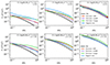 |
Fig. 8. Pressure profile as a function of the distance to the centre of the halos compared with the one predicted by HMx in dark grey at z = 0 (first row) and z = 1.18 (second row). Each panel represents a different mass bin and each colour is a different simulation: Horizon-AGN in red, Horizon-noAGN in purple, Horizon-Large in green, and Magneticum in blue. The error bars represent the error on the mean and are most of the time too small to be visible. |
Since the model’s free parameters are tailored to fit the response power spectrum, achieving a perfect agreement on pressure profiles is not guaranteed. Moreover, the influence of high masses, which contribute the most to the power spectrum, can alter even more the profiles of low-mass halos that contribute slightly to the power spectrum. The predicted profiles should be considered as the ones of effective halos, but it is still worth comparing the predicted and measured profiles, to understand power spectrum disparities. Let us describe more the high-mass bin which is the dominant part of the power spectrum. The difference observed in this bin could explain power spectrum differences. For example, at z = 0, all simulations (Horizon-AGN, Horizon-noAGN, Horizon-Large and Magneticum) have qualitatively similar pressure profiles (with more pronounced differences on the outer regions), containing more pressure than HMx. At z = 1.18, the Horizon-Large remains above the prediction, while Magneticum is under. On the left panel of Fig. 3, both Horizon-AGN and Horizon-noAGN power spectra also contain more power than HMx. However, on the right panel of Fig. 3, Horizon-Large power spectrum lies below HMx (with Magneticum showing relatively good agreement). These diverse behaviours suggest that profile differences alone cannot entirely account for observed power spectrum discrepancies. Additionally, we note that the lower-mass halos exhibit greater discrepancies, as anticipated.
To improve our analysis, it can be interesting to focus even more on high-mass halos and their impact on the tSZ properties. Future studies with larger volume simulations could provide a more comprehensive probe of these halos, which are quite rare in the Horizon suite, for example. Because of the current computational constraints, the resolution of such simulations cannot be as good as the one in Horizon-AGN, which can potentially introduce additional biases. Building large simulations with zoom-in capabilities targeting big halos to assess the fidelity of baryonic physics can be an avenue. This approach could offer a new perspective for such analysis, which is currently limited by the noise on the number of these halos.
5.3. Difference of the simulations
The simulations that we are analysing are different: they are run with different computational codes, different physics models, different resolutions, and different box sizes. Different choices in terms of the included physics and their modelisation methodology are made and can influence the obtained results. For example, in Mead et al. (2020), models were fitted against three BAHAMAS simulations, each containing different strengths of AGN feedback, yielding different values for the fitted parameters. In our simulations, with the different choices, the strength of feedback is also different, but other choices can lead to many other differences that are challenging to precisely identify and define.
Another critical aspect that can be evaluated is the cosmic variance of the simulation. To quantity this variance, we took 500 non-overlapping boxes extracted from the Horizon-Large simulation, each with a dimension of 100 h−1 Mpc. As the power spectrum depends a lot on the high-mass halos, we applied selection criteria to retain only boxes with maximal mass similar to the one in the Horizon-AGN and Horizon-noAGN simulations. This refinement yielded 363 non-overlapping boxes, from which we computed the pressure auto-power spectrum. We employed a constant binning in log space of k for our power spectrum, checking that the level of correlation between the bins is low. We then calculated a cumulative probability distribution function at each k to extract the values encompassing 68% of the signal. This approach allowed us to derive the lower and upper bounds of our error bars.
In Fig. 9 we show the binned mean power spectrum of these boxes, of the Horizon-noAGN simulation, and of the HMx prediction. The variance derived using the method described above is overlaid on the Horizon-noAGN simulation to represent the cosmic variance of such a simulation. We see that the error bars are non-Gaussian and of the same order of magnitude across different k ranges. They emphasize a tendency for a higher power spectrum than the one predicted by HMx.
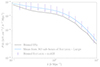 |
Fig. 9. Pressure auto-power spectrum in Horizon-noAGN in purple compared to HMx in dark grey and the mean over 363 sub-boxes of 100 h−1 Mpc from the Horizon-Large in blue. The purple error bars contain 68% around the mean of the 363 sub-boxes of the Horizon-Large (see the text for more information). They are applied to the Horizon-noAGN simulations to represent its variance. |
6. Conclusions
Within this paper, we compared the predicted (angular) power spectrum from HMx to the measurement from different simulations (Horizon-AGN, Horizon-noAGN, Horizon-Large and Magneticum). Using the HMx halo model, we predicted the pressure angular power spectra by integrating up to different redshifts or different masses. Our analysis first reveal that integration up to z = 4 (or even z = 3) accounts for more than 98% (96%) of the power. We also find that integrating up to 4 × 10¹⁵ h−1 M⊙ captures 97% of the signal, highlighting the significant contribution of higher masses to the power (this is also evident in Fig. 7 where we examined the power contribution from different mass bins at the level of the power spectrum). From these initial findings, we conclude that our comparison should focus on the redshift range between 0 and 4 and emphasize the importance of the highest mass range.
The main results of our analysis can be summarised in three points:
-
The comparison between the pressure power spectrum from different simulations with the one predicted by HMx for redshifts between z = 0 and z = 4.25 (Fig. 3), reveals a qualitative conclusion which is consistent across all simulations: at low redshift, there is a qualitative agreement between measurements and predictions but discrepancies increase with higher redshifts.
-
A similar trend is observed for the matter-pressure power spectrum (Fig. 4), although the discrepancies are less pronounced due to better agreement in the matter-auto power spectra. It is important to note that when working with cross-correlation such as the weak lensing-tSZ one, sensitivity extends only up to a redshift ∼2. This range is where HMx shows relatively good agreement.
-
The comparison between the predicted and measured pressure angular power spectrum reveals differences ranging from 20 to 50% across all simulations.
To understand the origin of the discrepancies, we explored the limitations inherent to the halo model:
-
we observe that the excess of power in the HMx prediction is dominated by the one-halo term at high k and by the two-halo term at low k (Fig. 6),
-
we investigated the contribution of power from within and outside one virial radius of halos in the simulations at different redshifts (Fig. 6). At lower redshifts, the majority of power originates from within halos, indicating compatibility with the halo model assumption. However, at higher redshift (e.g. z ∼ 3), a substantial portion of the power comes from regions outside one virial radius of halos, highlighting a limitation of the halo model to capture this phenomenon,
-
we compared the pressure profiles across different mass bins and redshifts, as the pressure profile is the main property of the halo model (Fig. 8). While differences were expected due to the halo model being fitted at the level of the response power spectrum, it was informative to observe the behaviour and degeneracies. Across most mass and redshift ranges, the simulations exhibit higher power levels and distinct profile shapes compared to the predictions.
Enhancing the robustness of predictions could be achieved by developing a halo model that more accurately reflects the physics within simulations. This could involve calibrations on simulations at the level of individual properties, such as the pressure profile. Additionally, to apply a halo model framework in cosmological analyses, calibrating the model with real data would be beneficial. Such approaches come with inherent challenges, such as the parameter measurement methodologies. Exploring different parametrisations that better align with these properties may help determine whether an accurate match at the component level would lead to a robust power spectrum prediction. Employing larger and better-resolved simulations, which include more massive halos, can also address some limitations of the halo model, particularly by enhancing our understanding of the tSZ effect and the behaviour of high-mass halos across different redshifts. Another significant avenue for exploration is investigating the variability of the tSZ power spectrum under different cosmologies. This includes assessing the influence of cosmological parameters that impact the growth of structures, such as the quantity of baryonic matter or the dark energy) equation of state.
Acknowledgments
We thank Klaus Dolag for giving us access to the Magneticum simulations and the useful discussions. This work has made use of the Infinity Cluster hosted by Institut d’Astrophysique de Paris. We thank Stéphane Rouberol for running smoothly this cluster for us. EA, KB, and YD acknowledge support by the CNES, the French National Space Agency. EA and PRS are supported in part by a PhD Joint Program between the CNRS and the University of Arizona. EK is supported in part by Department of Energy grant DE-SC0020247, the David and Lucile Packard Foundation and an Alfred P. Sloan Research Fellowship. The contributions of the authors, classified according to the CRediT (Contribution Roles Taxonomy) (https://authorservices.wiley.com/author-resources/Journal-Authors/open-access/credit.html) system, were as follows: Emma Ayçoberry: Conceptualization; Formal Analysis; Software; Validation; Visualization; Writing – Original Draft Preparation. Pranjal R. S.: Formal Analysis; Validation; Visualization; Writing – Review & Editing. Karim Benabed: Conceptualization; Validation; Writing – Original Draft Preparation. Yohan Dubois: Conceptualization; Data Curation; Software; Validation; Writing – Original Draft Preparation. Elisabeth Krause: Conceptualization; Validation; Writing – Review & Editing. Tim Eifler: Validation; Writing – Review & Editing.
References
- Aubert, D., Pichon, C., & Colombi, S. 2004, MNRAS, 352, 376 [Google Scholar]
- Battaglia, N., Bond, J. R., Pfrommer, C., & Sievers, J. L. 2012, ApJ, 758, 75 [NASA ADS] [CrossRef] [Google Scholar]
- Beckmann, R. S., Devriendt, J., Slyz, A., et al. 2017, MNRAS, 472, 949 [NASA ADS] [CrossRef] [Google Scholar]
- Bleem, L. E., Crawford, T. M., Ansarinejad, B., et al. 2022, ApJS, 258, 36 [NASA ADS] [CrossRef] [Google Scholar]
- Bolliet, B., Comis, B., Komatsu, E., & Macías-Pérez, J. F. 2018, MNRAS, 477, 4957 [NASA ADS] [CrossRef] [Google Scholar]
- Bolliet, B., Kusiak, A., McCarthy, F., et al. 2023, ArXiv e-prints [arXiv:2310.18482] [Google Scholar]
- Bryan, G. L., & Norman, M. L. 1998, ApJ, 495, 80 [NASA ADS] [CrossRef] [Google Scholar]
- Chisari, N. E., Richardson, M. L. A., Devriendt, J., et al. 2018, MNRAS, 480, 3962 [Google Scholar]
- Davis, O., Devriendt, J., Colombi, S., Silk, J., & Pichon, C. 2011, MNRAS, 413, 2087 [NASA ADS] [CrossRef] [Google Scholar]
- Debackere, S. N. B., Schaye, J., & Hoekstra, H. 2020, MNRAS, 492, 2285 [Google Scholar]
- Dolag, K., & Stasyszyn, F. 2009, MNRAS, 398, 1678 [NASA ADS] [CrossRef] [Google Scholar]
- Dolag, K., Komatsu, E., & Sunyaev, R. 2016, MNRAS, 463, 1797 [Google Scholar]
- Dubois, Y., & Teyssier, R. 2008, A&A, 477, 79 [NASA ADS] [CrossRef] [EDP Sciences] [Google Scholar]
- Dubois, Y., Devriendt, J., Slyz, A., & Teyssier, R. 2012, MNRAS, 420, 2662 [Google Scholar]
- Dubois, Y., Pichon, C., Welker, C., et al. 2014, MNRAS, 444, 1453 [Google Scholar]
- Dubois, Y., Peirani, S., Pichon, C., et al. 2016, MNRAS, 463, 3948 [Google Scholar]
- Eifler, T., Fang, X., Krause, E., et al. 2024, ArXiv e-prints [arXiv:2411.04088] [Google Scholar]
- Fang, X., Krause, E., Eifler, T., et al. 2024, MNRAS, 527, 9581 [Google Scholar]
- Fedeli, C. 2014, JCAP, 2014, 028 [CrossRef] [Google Scholar]
- Ferragamo, A., de Andres, D., Sbriglio, A., et al. 2023, MNRAS, 520, 4000 [NASA ADS] [CrossRef] [Google Scholar]
- Gonzalez, A. H., Sivanandam, S., Zabludoff, A. I., & Zaritsky, D. 2013, ApJ, 778, 14 [Google Scholar]
- Haardt, F., & Madau, P. 1996, ApJ, 461, 20 [Google Scholar]
- Hinshaw, G., Larson, D., Komatsu, E., et al. 2013, ApJS, 208, 19 [Google Scholar]
- Hirschmann, M., Dolag, K., Saro, A., et al. 2014, MNRAS, 442, 2304 [Google Scholar]
- Holz, D. E., & Perlmutter, S. 2012, ApJ, 755, L36 [NASA ADS] [CrossRef] [Google Scholar]
- Komatsu, E., & Kitayama, T. 1999, ApJ, 526, L1 [NASA ADS] [CrossRef] [Google Scholar]
- Komatsu, E., & Seljak, U. 2001, MNRAS, 327, 1353 [Google Scholar]
- Komatsu, E., & Seljak, U. 2002, MNRAS, 336, 1256 [NASA ADS] [CrossRef] [Google Scholar]
- Komatsu, E., Smith, K. M., Dunkley, J., et al. 2011, ApJS, 192, 18 [Google Scholar]
- Laureijs, R., Amiaux, J., Arduini, S., et al. 2011, ArXiv e-prints [arXiv:1110.3193] [Google Scholar]
- Le Brun, A. M. C., McCarthy, I. G., Schaye, J., & Ponman, T. J. 2014, MNRAS, 441, 1270 [NASA ADS] [CrossRef] [Google Scholar]
- Le Brun, A. M. C., McCarthy, I. G., & Melin, J.-B. 2015, MNRAS, 451, 3868 [NASA ADS] [CrossRef] [Google Scholar]
- Lee, B. K. K., Coulton, W. R., Thiele, L., & Ho, S. 2022, MNRAS, 517, 420 [NASA ADS] [CrossRef] [Google Scholar]
- Ma, Y.-Z., Van Waerbeke, L., Hinshaw, G., et al. 2015, JCAP, 2015, 046 [CrossRef] [Google Scholar]
- Maniyar, A., Béthermin, M., & Lagache, G. 2021, A&A, 645, A40 [NASA ADS] [CrossRef] [EDP Sciences] [Google Scholar]
- McCarthy, I. G., Le Brun, A. M. C., Schaye, J., & Holder, G. P. 2014, MNRAS, 440, 3645 [NASA ADS] [CrossRef] [Google Scholar]
- McCarthy, I. G., Schaye, J., Bird, S., & Le Brun, A. M. C. 2017, MNRAS, 465, 2936 [Google Scholar]
- McCarthy, I. G., Bird, S., Schaye, J., et al. 2018, MNRAS, 476, 2999 [NASA ADS] [CrossRef] [Google Scholar]
- McCarthy, I. G., Salcido, J., Schaye, J., et al. 2023, MNRAS, 526, 5494 [NASA ADS] [CrossRef] [Google Scholar]
- Mead, A. J., Tröster, T., Heymans, C., Van Waerbeke, L., & McCarthy, I. G. 2020, A&A, 641, A130 [EDP Sciences] [Google Scholar]
- Menanteau, F., González, J., Juin, J.-B., et al. 2010, ApJ, 723, 1523 [Google Scholar]
- Mo, H. J., & White, S. D. M. 1996, MNRAS, 282, 347 [Google Scholar]
- Moser, E., Battaglia, N., Nagai, D., et al. 2022, ApJ, 933, 133 [NASA ADS] [CrossRef] [Google Scholar]
- Osato, K., & Takada, M. 2021, Phys. Rev. D, 103, 063501 [NASA ADS] [CrossRef] [Google Scholar]
- Osato, K., Shirasaki, M., Miyatake, H., et al. 2020, MNRAS, 492, 4780 [NASA ADS] [CrossRef] [Google Scholar]
- Pandey, S., Lehman, K., Baxter, E. J., et al. 2023, MNRAS, 525, 1779 [CrossRef] [Google Scholar]
- Perotto, L., Adam, R., Ade, P., et al. 2023, ArXiv e-prints [arXiv:2310.04553] [Google Scholar]
- Plagge, T., Benson, B. A., Ade, P. A. R., et al. 2010, ApJ, 716, 1118 [Google Scholar]
- Planck Collaboration XXIX. 2014, A&A, 571, A29 [NASA ADS] [CrossRef] [EDP Sciences] [Google Scholar]
- Planck Collaboration XVI. 2014, A&A, 571, A16 [NASA ADS] [CrossRef] [EDP Sciences] [Google Scholar]
- Planck Collaboration XXII. 2016, A&A, 594, A22 [NASA ADS] [CrossRef] [EDP Sciences] [Google Scholar]
- Refregier, A., & Teyssier, R. 2002, Phys. Rev. D, 66, 043002 [NASA ADS] [CrossRef] [Google Scholar]
- Refregier, A., Komatsu, E., Spergel, D. N., & Pen, U.-L. 2000, Phys. Rev. D, 61, 123001 [CrossRef] [Google Scholar]
- Sadeh, S., Rephaeli, Y., & Silk, J. 2007, MNRAS, 380, 637 [NASA ADS] [CrossRef] [Google Scholar]
- Schaye, J., Dalla Vecchia, C., Booth, C. M., et al. 2010, MNRAS, 402, 1536 [Google Scholar]
- Seljak, U., Burwell, J., & Pen, U.-L. 2001, Phys. Rev. D, 63, 063001 [CrossRef] [Google Scholar]
- Sheth, R. K., & Tormen, G. 1999, MNRAS, 308, 119 [Google Scholar]
- Sheth, R. K., Mo, H. J., & Tormen, G. 2001, MNRAS, 323, 1 [NASA ADS] [CrossRef] [Google Scholar]
- Sorini, D., Bose, S., Pakmor, R., et al. 2025, MNRAS, 536, 728 [Google Scholar]
- Spacek, A., Richardson, M. L. A., Scannapieco, E., et al. 2018, ApJ, 865, 109 [NASA ADS] [CrossRef] [Google Scholar]
- Springel, V., & Hernquist, L. 2003, MNRAS, 339, 289 [Google Scholar]
- Springel, V., White, M., & Hernquist, L. 2001, ApJ, 549, 681 [CrossRef] [Google Scholar]
- Springel, V., White, S. D. M., Jenkins, A., et al. 2005, Nature, 435, 629 [Google Scholar]
- Sunyaev, R. A., & Zeldovich, Y. B. 1970, Ap&SS, 7, 3 [NASA ADS] [Google Scholar]
- Sutherland, R. S., & Dopita, M. A. 1993, ApJS, 88, 253 [Google Scholar]
- Teyssier, R. 2002, A&A, 385, 337 [CrossRef] [EDP Sciences] [Google Scholar]
- Tornatore, L., Borgani, S., Springel, V., et al. 2003, MNRAS, 342, 1025 [NASA ADS] [CrossRef] [Google Scholar]
- Tornatore, M., Maier, G., & Pattavina, A. 2006, J. Opt. Netw., 5, 858 [NASA ADS] [CrossRef] [Google Scholar]
- Tröster, T., Mead, A. J., Heymans, C., et al. 2022, A&A, 660, A27 [CrossRef] [EDP Sciences] [Google Scholar]
- Van Waerbeke, L., Hinshaw, G., & Murray, N. 2014, Phys. Rev. D, 89, 023508 [Google Scholar]
- Villaescusa-Navarro, F. 2018, Astrophysics Source Code Library [record ascl:1811.008] [Google Scholar]
- Vogelsberger, M., Genel, S., Springel, V., et al. 2014, MNRAS, 444, 1518 [Google Scholar]
- Waizmann, J. C., & Bartelmann, M. 2009, A&A, 493, 859 [NASA ADS] [CrossRef] [EDP Sciences] [Google Scholar]
- Wiersma, R. P. C., Schaye, J., Theuns, T., Dalla Vecchia, C., & Tornatore, L. 2009, MNRAS, 399, 574 [NASA ADS] [CrossRef] [Google Scholar]
Appendix A: Power spectrum computation
A.1. Power spectrum computation in the Horizon suite of simulations
To obtain the different power spectra from the simulations, we followed different procedures for the Horizon and Magneticum suite of simulations.
A.1.1. Power spectrum computation in the Horizon suite of simulations
To compute the power spectra in the Horizon suite of simulations, we first needed to project the component of interest onto a uniform three-dimensional grid. The matter component is the sum of the dark matter, stars, and gas. DM and stars were projected with a cloud-in-cell interpolation on the grid. Gas quantities were already on the regular Cartesian grid and we directly used the values of mass or pressure from the corresponding level of refinement. The simulations provided the total gas pressure, which we can easily modify to obtain the electron pressure, assuming local thermodynamic equilibrium between ions and electrons for a fully ionized gas, that is:
 (A.1)
(A.1)
where P is the total gas pressure, μ (μe) is the mean molecular weight for gas (electron) particles. We projected our quantity into a 5123 grid, allowing us to reach a Nyquist frequency (kNy = π × Nmesh/Lbox) of kNy ∼ 16 h Mpc−1 for Horizon-AGN and Horizon-noAGN and up to kNy ∼ 1.8 h Mpc−1 for Horizon-Large. To obtain the angular power spectrum, it was beneficial to project Horizon-Large into a 10243 grid to achieve kNy ∼ 3.6 h Mpc−1.
Once the quantity is projected, we used the Pylians python package (Villaescusa-Navarro 2018) to compute the 3D auto- and cross-power spectra deconvolved by the CIC mass-assignment scheme.
A.2. Power spectrum computation in Magneticum
For the Magneticum simulation, we assigned each gas particle (labelled by i) an electron pressure Pe, i according to the ideal gas law
 (A.2)
(A.2)
 (A.3)
(A.3)
where Ti is the particle temperature, Vcell is the cell volume, Ne, i is the number of free electrons, Mi is the SPH particle mass, μe, i = 2/(2 − Yi) is the mean mass per electron and Yi is the Helium fraction.
We used Pylians to project the electron pressure onto a 10243 mesh based on the CIC assignment scheme and then measured the power spectrum. We thus achieve kNy ∼ 3.6 h Mpc−1.
All Figures
|
Fig. 1. Predicted pressure angular power spectrum when integrating up to different redshifts in different colours (on the left) or between z = 0.02 and z = 10 for different maximal mass in different colours (on the right) as a function of the angular scale ℓ. |
| In the text | |
|
Fig. 2. Halo mass function at z = 0 for the Horizon-AGN, Horizon-noAGN, Horizon-Large, and Magneticum simulations in red, purple, green, and blue, respectively, with their associated Poisson noise as error bar. Each mass function is computed up to the maximal halo mass in the corresponding simulation. The analytical mass function from Sheth & Tormen (1999) is shown in black for comparison. Vertical lines indicate the minimum halo mass accessible in each simulation, defined as 100 times the dark matter mass resolution. The lower limits for Horizon-AGN and Horizon-noAGN are identical. |
| In the text | |
|
Fig. 3. Pressure auto-power spectrum as a function of redshift. The left panel shows the results for simulations with a box size of 100 h−1 Mpc, thus Horizon-AGN in dashed line compared to HMx in solid line, and Horizon-noAGN at z = 0 in dotted line. The right panel shows the results for simulations with a box size of 896 h−1 Mpc, thus Magneticum in dashed line compared to HMx in solid line, and Horizon-Large at z = 0 in dotted line. The power spectra go from z = 0 in dark blue to z = 4.25 in yellow. |
| In the text | |
|
Fig. 4. Matter-pressure power spectrum as a function of redshift. The left panel shows the results for simulations with a box size of 100 h−1 Mpc, thus Horizon-AGN in dashed line compared to HMx in solid line, and Horizon-noAGN at z = 0 in dotted line. The right panel shows the results for simulations with a box size of 896 h−1 Mpc, thus Magneticum in dashed line compared to HMx in solid line, and Horizon-Large at z = 0 in dotted line. The power spectra go from z = 0 in dark blue to z = 4.25 in yellow. |
| In the text | |
|
Fig. 5. Pressure angular power spectrum integrated between z = 0 and z = 4 for the different simulations in different colours and HMx in dark grey. The left panel shows the results for simulation with a box size of 100 h−1 Mpc, thus Horizon-AGN in red and Horizon-noAGN in purple. The right panel shows the results for simulation with a box size of 896 h−1 Mpc, thus Horizon-Large in green and Magneticum in blue. |
| In the text | |
|
Fig. 6. Pressure auto-power spectrum as a function of redshift in the different panels. For every redshift, we show the power spectrum of Horizon-AGN in a coloured dashed line, the HMx prediction in a coloured full line, the predicted one-halo term in a coloured thin line, and the predicted two-halo term in a coloured dotted-dashed line. We superimpose the pressure auto-power spectrum within (without) one virial radius in a grey full line (grey dotted-dashed line). On the left, we show the result for z = 0.02, on the middle for z = 1.16, and on the right for z = 3.01. |
| In the text | |
|
Fig. 7. Pressure auto-power spectrum of the total Horizon-AGN simulation in red compared to the signal coming from within one virial radius of different mass bin. The highest mass bin is in dark brown and corresponds to the mass bin 14 < log(Mv/M⊙ h−1) < 15, we then decrease of one dex for every curve until reaching the lowest mass bin in yellow, which corresponds to the mass bin log(Mv/M⊙ h−1) < 10. |
| In the text | |
|
Fig. 8. Pressure profile as a function of the distance to the centre of the halos compared with the one predicted by HMx in dark grey at z = 0 (first row) and z = 1.18 (second row). Each panel represents a different mass bin and each colour is a different simulation: Horizon-AGN in red, Horizon-noAGN in purple, Horizon-Large in green, and Magneticum in blue. The error bars represent the error on the mean and are most of the time too small to be visible. |
| In the text | |
|
Fig. 9. Pressure auto-power spectrum in Horizon-noAGN in purple compared to HMx in dark grey and the mean over 363 sub-boxes of 100 h−1 Mpc from the Horizon-Large in blue. The purple error bars contain 68% around the mean of the 363 sub-boxes of the Horizon-Large (see the text for more information). They are applied to the Horizon-noAGN simulations to represent its variance. |
| In the text | |
Current usage metrics show cumulative count of Article Views (full-text article views including HTML views, PDF and ePub downloads, according to the available data) and Abstracts Views on Vision4Press platform.
Data correspond to usage on the plateform after 2015. The current usage metrics is available 48-96 hours after online publication and is updated daily on week days.
Initial download of the metrics may take a while.