| Issue |
A&A
Volume 693, January 2025
|
|
|---|---|---|
| Article Number | A94 | |
| Number of page(s) | 15 | |
| Section | Extragalactic astronomy | |
| DOI | https://doi.org/10.1051/0004-6361/202452006 | |
| Published online | 07 January 2025 | |
Non-thermal emission in galaxy groups at extremely low frequency: The case of A1213
1
INAF – Istituto di Radioastronomia, Via P. Gobetti 101, 40129 Bologna, Italy
2
Cavendish Laboratory – Astrophysics Group, University of Cambridge, 19 JJ Thomson Avenue, Cambridge CB3 0HE, United Kingdom
3
Kavli Institute for Cosmology, University of Cambridge, Madingley Road, Cambridge CB3 0HA, United Kingdom
4
Centre for Radio Astronomy Techniques and Technologies, Department of Physics and Electronics, Rhodes University, PO Box 94 Makhanda 6140, South Africa
5
South African Radio Astronomy Observatory, Black River Park North, 2 Fir St, Cape Town 7925, South Africa
6
Department of Astronomy, University of Geneva, Ch. d’Ecogia 16, 1290 Versoix, Switzerland
7
Leiden Observatory, Leiden University, PO Box 9513 2300 RA Leiden, The Netherlands
8
INAF, IASF-Milano, Via A.Corti 12, 20133 Milano, Italy
9
Hamburger Sternwarte, Universität Hamburg, Gojenbergsweg 112, 21029 Hamburg, Germany
10
National Centre for Radio Astrophysics, Tata Institute of Fundamental Research, Pune 411007, India
⋆ Corresponding author; This email address is being protected from spambots. You need JavaScript enabled to view it.
Received:
27
August
2024
Accepted:
22
November
2024
Abstract
Context. Galaxy clusters and groups are the last link in the chain of hierarchical structure formation. Their environments can be significantly affected by outbursts from active galactic nuclei (AGN), especially in groups where the medium density is lower and the gravitational potential is shallower. Thus, interaction between AGN and group weather can greatly affect their evolution.
Aims. We investigate the non-thermal radio emission in Abell 1213, a galaxy group that is part of a larger sample of ∼50 systems (X-GAP) recently explored in XMM-Newton observations.
Methods. We exploited proprietary LOFAR 54 MHz and uGMRT 380 MHz observations, complementing them with 144 MHz LOFAR survey and XMM-Newton archival data.
Results. A1213 hosts a bright AGN associated with one of the central members, 4C 29.41, which was previously optically identified as a dumb-bell galaxy. Observations at 144 MHz at a resolution of 0.3″ have allowed us to resolve the central radio galaxy. From this source, a ∼500 kpc-long tail extends in the north-east direction. Our analysis suggests that the tail likely originated from a past outburst of 4C 29.41 and its current state might be the result of the interaction with the surrounding environment. The plateau of the spectral index distribution in the easternmost part of the tail suggests mild particle re-acceleration, which could have re-energised seed electrons from the past activity of the AGN. While we do observe a spatial and physical correlation of the extended, central emission with the thermal plasma (which might hint at a mini-halo), the current evidence cannot prove this conclusively.
Conclusions. A1213 is only the first group among the X-GAP sample that we have been able to investigate via low-frequency radio observations. Its complex environment once again demonstrates the significant impact that the interplay between thermal and non-thermal processes can exert on galaxy groups.
Key words: galaxies: active / galaxies: groups: general / galaxies: groups: individual: A1213
© The Authors 2025
 Open Access article, published by EDP Sciences, under the terms of the Creative Commons Attribution License (https://creativecommons.org/licenses/by/4.0), which permits unrestricted use, distribution, and reproduction in any medium, provided the original work is properly cited.
This article is published in open access under the Subscribe to Open model. This email address is being protected from spambots. You need JavaScript enabled to view it. to support open access publication.
1. Introduction
In recent decades, it has become clear that jets from active galactic nuclei (AGN) can strongly affect the surrounding medium across a vast range (∼pc to ∼Mpc) of physical scales (e.g. Clark et al. 1997; Zanni et al. 2005; Morganti et al. 2013; Brienza et al. 2023). This is especially relevant in galaxy clusters and groups, where jets can excavate through the intra-cluster or intra-group medium (ICM or IGrM), creating cavities (e.g. Brüggen & Kaiser 2002; Bîrzan et al. 2004; Rafferty et al. 2006), uplifting metal-rich gas (e.g. Ettori et al. 2013; Gastaldello et al. 2021), and inducing turbulence and shocks (e.g. Brunetti & Lazarian 2007).
While we primarily observe Faranoff-Riley I (FRI) sources at the centre of galaxy clusters (likely because initially-relativistic jets collect material and slow down while travelling through the high-density ICM), poorer environments (e.g. those of galaxy groups) often host FRII radio galaxies (Yates et al. 1989; Hill & Lilly 1991). Nevertheless, it is not rare to also find FRII in rich clusters (see e.g. Ledlow & Owen 1995), as evidence seems to show that the FRI-FRII dichotomy might also be linked to the super-massive black hole (SMBH) accretion mode (Ghisellini & Celotti 2001; Marchesini et al. 2004). Jetted AGN are indeed observed even in massive galaxies, which are predominantly hosted in richer environments (Brienza et al. 2023). Feedback from these AGN jets therefore plays a fundamental role in the evolution of clusters and groups, promoting or preventing star formation, and regulating the cooling of the ICM and IGrM (see e.g. McNamara & Nulsen 2012 for a review).
Nevertheless, the non-thermal emission observed in clusters and groups is not only associated to radio galaxies (see e.g. reviews by Feretti et al. 2012; van Weeren et al. 2019). Low-frequency instruments such as the Giant Metrewave Radio Telescope (GMRT, Gupta et al. 2017) and the LOw-Frequency ARray (LOFAR, van Haarlem et al. 2013) have helped shed light on diffuse, ∼Mpc-scale synchrotron emission that was originally detected by higher frequency surveys (Rengelink et al. 1997; Giovannini et al. 1999). An example are radio halos, whose synchrotron spectra1 usually show a rather uniform spectral index with α ∼ −1.2 (see e.g. review by van Weeren et al. 2019); although, we note that this value was mainly estimated from high-frequency detections in massive systems.
A growing number of recent detections by LOFAR and uGMRT, which has searched for halos with relatively steep spectra (α < −1.5, see e.g. Bonafede et al. 2012; Wilber et al. 2018; Di Gennaro et al. 2021; Bruno et al. 2021; Edler et al. 2022; Pasini et al. 2022a, 2024), combined with gamma-ray constraints (e.g. Ackermann et al. 2010; Zandanel & Ando 2014; Osinga et al. 2024), points to a leptonic origin, where seed electrons get re-accelerated by turbulence induced by major mergers (Brunetti et al. 2001; Cassano & Brunetti 2005; Brunetti & Lazarian 2011). This is in line with early predictions about the cosmic ray (CR) proton energy budget (Brunetti et al. 2008; Brunetti & Lazarian 2011).
Radio relics are instead observed at the periphery of merging systems and always show a certain degree of polarisation and elongated morphology (van Weeren et al. 2010), with their orientation being usually orthogonal to that of the merger axis. The spectral index distribution shows a gradient, with steeper values in the region closer to the cluster centre, and flatter indices on the outer side (e.g. Bonafede et al. 2012; de Gasperin et al. 2014). For these reasons, the most promising formation models invoke re-acceleration of seed electrons by shocks (Brunetti & Lazarian 2007; Kang 2017) which (similarly to turbulence) are generated by major mergers.
While the vast majority of studies of continuum radio emission have been carried out on massive galaxy clusters, the mass regime of galaxy groups (M500 < 1014 M⊙) is still largely unexplored. In that direction, Complete Local-Volume Groups Sample (CLoGS) studies have explored the multi-wavelength (O’Sullivan et al. 2017; O’Sullivan et al. 2018; Kolokythas et al. 2018, 2019, 2022) properties of 53 nearby central brightest group galaxies (BGGs), examining their energy output based on an unbiased set of low-mass systems.
The impact of powerful AGN outbursts in groups, which may extend beyond the virial radius, has a significant effect on their evolution. Any difference with respect to more massive systems should therefore be reflected even in the properties of central radio galaxies (Pasini et al. 2020, 2021, 2022b) and of the intra-group medium (IGrM, see e.g. review by Morganti et al. 2013).
In light of these issues, the XMM-Newton Group AGN Project (X-GAP, Eckert et al. 2024) aims to quantify the impact of AGN feedback in a complete sample of 49 galaxy groups, which will be observed with XMM-Newton for a total of ∼852 ks2. The same systems have (or will be) also been observed by LOFAR at 54 (de Gasperin et al. 2023) and 144 MHz (Shimwell et al. 2022), while a smaller sub-sample will also have dedicated uGMRT observations.
Abell 1213 (hereafter A1213) is a galaxy group3 at z = 0.0748 (Abell et al. 1989) that is part of the X-GAP sample. It lies on the edge between the cluster and group mass regimes (M200 = (1.54 ± 0.25)×1014 M⊙, Boschin et al. 2023, hereafter B23). An early work by Giovannini et al. (2009) first claimed the presence of diffuse emission, using 1.4 GHz observations at ∼35″ resolution by the Very Large Array (VLA)4 to explain an elongated trail of emission lying to the east of one of the brightest group members, 4C 29.41 (Jones & Forman 1999). These authors classified it as a powerful FRII radio galaxy. The radio emission of this galaxy shows signs (in projection) of a physical association with the diffuse cluster plasma, which was labelled as a radio halo in Giovannini et al. (2009). The optical galaxy identified with the radio source 4C 29.41 = B2 1113+29 is a dumb-bell galaxy (Fanti et al. 1982). B23 discussed the presence of two nearby galaxies: ID 467 and ID 468. The radio emission is from ID 467. The two galaxies show an excess of intra-cluster light likely due to interaction and should be considered a couple of bright galaxies. On the other hand, they identified the BGG with an elliptical galaxy that lies ∼50 kpc west to 4C 29.41. This object hosts a flat-spectrum radio source, although its morphology is rather compact (∼15 kpc size) and appears to be disconnected from the more extended emission of 4C 29.41.
B23 also studied the dynamics of this system, making use of optical data from the Sloan Digital Sky Survey (SDSS, York et al. 2000). Thanks to a total of 143 spectroscopic galaxy members, they found that A1213 is a disturbed system consisting of several smaller galaxy groups, most likely merging together on the NE-SW direction. They support this hypothesis through an archival X-ray observation by XMM-Newton, which shows a clear elongated morphology of the IGrM in the same direction. Furthermore, through public 144 MHz LOFAR observations by the LOFAR Two-Metre Sky Survey (LoTSS, Shimwell et al. 2019, 2022), they confirm the presence of large-scale (∼500 kpc) radio emission extending eastwards from 4C 29.41, but which does not show the typical properties and morphology of a radio halo. In fact, its surface brightness distribution describes an elongated and filamentary structure, which appears physically unrelated to the thermal plasma. Instead, B23 proposed that this trail of emission is a radio relic, supporting this hypothesis through a gradient in the spectral index map between 144 MHz and 1.4 GHz, which steepens from north to south. Finally, they interpret the presence of fragmented patches of emission around the BGG as a faint radio halo candidate.
In this study, thanks to the availability of new low-frequency radio data, we propose a new interpretation on this very peculiar system, which is the first within the X-GAP sample that we have been able study in detail thanks to the LOFAR and uGMRT proprietary data. We performed a thorough analysis of the radio emission, making use of a wide range of frequencies: from LOFAR Low Band Antenna (LBA) at 54 MHz and LOFAR High Band Antenna (HBA) at 144 MHz to uGMRT observations at 380 MHz. Thanks to the international stations of LOFAR, we have been able to reach an unprecedented angular resolution of ∼0.3″ at 144 MHz for this system, which allowed us to fully resolve the central radio galaxy. Furthermore, we examined the properties of the large-scale environment by performing a comparison between the non-thermal (radio) and the thermal (X-ray) emission, using an archival XMM-Newton observation.
Throughout this work, we adopted a ΛCDM cosmology with H0 = 70 km s−1 Mpc−1, ΩΛ = 0.7 and ΩM = 1 − ΩΛ = 0.3. Unless otherwise reported, errors are at 68% confidence level (1σ). At a redshift of z = 0.0478 the luminosity distance is 212 Mpc, leading to a conversion of 1″ = 0.94 kpc.
2. Data calibration and analysis
2.1. LBA observation
A1213 has been observed by LOFAR in LBA_SPARSE_EVEN configuration on 2 November 2022, for a total of 10 hours, as part of the proprietary project DDT18_001 (P.I. H. Edler). The frequency range is 42 − 66 MHz, with 54 MHz central frequency and 64 channels per sub-band, where each sub-band has a frequency width of 195 kHz. The observation has been calibrated through the automated Pipeline for LOFAR LBA (PiLL), which is extensively described in de Gasperin et al. (2019, 2021, 2023). We summarise here the main steps.
First, after a round of radio frequency interferences (RFI) flagging and data averaging, the bandpass and phase solutions for the calibrator (3C 295) can be estimated from a calibrator model included in PiLL and then transferred to the target. Direction-independent calibration then corrects for first-order ionospheric delays, Faraday rotation, and second-order beam errors. Direction-dependent calibration is performed by adopting the facet approach (van Weeren et al. 2016): all the sources are subtracted from the visibilities, then the brightest source is re-added and solutions for this direction are determined. This step is repeated for every sufficiently bright source (DD-calibrator) in the field of view (FoV). The field is then divided into facets, based on the position of DD-calibrators, and the same solutions for each of them are applied to every source in the corresponding facet. These steps are done through DDFacet (Tasse et al. 2018).
Finally, we can further improve the correction of direction-dependent ionospheric effects by performing the same extraction process first adopted for HBA observations in van Weeren et al. (2021) and described for LBA in Pasini et al. (2022a). We selected a small region (∼15′) around our target of interest, A1213. All sources outside this region were subtracted and (if necessary) the phase centre of the observation is shifted to the target position. The data were averaged in time and frequency to reduce the overall size and smear the signal of improperly subtracted off-axis sources. A primary beam correction at the new phase centre was applied through image domain gridding (IDG, van der Tol et al. 2018). Self-calibration cycles then helped to reduce the noise and improve the image quality.
Imaging was carried out through WSClean (Offringa et al. 2014) by applying suitable weighting and tapering of the visibilities in order to obtain images at different resolutions. To enhance the visualisation of extended diffuse emission and avoid contamination by spurious sources, we performed the subtraction of compact sources as follows. First, a high-resolution image is produced by cutting visibilities below 800 λ, which roughly corresponds to a largest angular size (LAS) of 266″ and a largest linear size of 250 kpc at the group redshift. This threshold was chosen (after a visual inspection of the images), so that only sources below this LLS, roughly corresponding to twice the size of the central AGN, end up imaged. The clean components of these sources are then stored as a model through the predict option of WSClean and subtracted from the original datasets. After this approach, images only show extended emission with LLS > 250 kpc, while smaller sources get excluded. Flux density uncertainties are conservatively estimated to be 10%, which is similar to LoLSS (de Gasperin et al. 2021, 2023).
2.2. HBA observation
A1213 was observed by LOFAR at 144 MHz as part of the second Data Release of LoTSS DR2 (Shimwell et al. 2022). The target is covered by two survey pointings, P168+30 and P171+30, for a total of 16 hours (with 8 hours per pointing, i.e. 8 hours longer than the observation used in B23, which only covers P168+30). The two pointings were independently calibrated making use of a set of automated pipelines developed to calibrate LOFAR HBA data: prefactor (van Weeren et al. 2016; Williams et al. 2016) and ddf-pipeline (Tasse et al. 2021). The algorithm performs flagging of radio frequency interference (RFI), averages the data based on time and frequency, and corrects for direction-independent effects such as clock offsets, complex gains, and phase delays. The direction-dependent calibration follows the same steps listed above for LBA. Finally, an extraction is performed on the two separated datasets, similarly to the process detailed in the previous section, as well as imaging and compact-sources subtraction with the same threshold of 250 kpc used for the lower frequency. The flux density scale was aligned with the LoTSS-DR2 data release, where the flux calibration uncertainty is estimated to be ∼10% (Hardcastle et al. 2021). With respect to the image presented in B23, which is a simple cutout of the source in the pointing P168+30, our reprocessed image has better signal-to-noise ratio (S/N), as it combines two survey pointings. For a comparison, the image in B23 has a rms noise of ∼150 μJy beam−1, while we reach ∼100 μJy beam−1. Furthermore, the extraction has further improved the self-calibration of the source, eliminating most of the artefacts visible in the non-processed survey image.
The processing for the full European array of LOFAR was done using the LOFAR-VLBI pipeline5 described by Morabito et al. (2022). It deviates from the Dutch array processing described above, following the ddf-pipeline step. From the calibrated data (with their calibration solutions applied from prefactor and the ddf-pipeline solutions, applicable for the Dutch stations only; except for the bandpass and ionospheric rotation measure, RM), the phase centre of the data was then shifted to the coordinates of 4C 29.41 and averaged. We then apply the facetselfcal procedure (van Weeren et al. 2021), where we combined the core stations in the Dutch array into a ‘super station’, allowing for an accurate anchor for the self-calibration of the longer baselines. This limits the largest angular scale to 71 arcsec. We began a self-calibration cycle by using a starting sky model predicted from a VLA L-band image of 4C 29.41, taken from the NVAS archive6. Several iterations of phase and complexgain self-calibration were performed, giving a final image with an RMS background noise of 50 μJy beam−1 at an angular resolution of 0.36″ × 0.19″.
To view the larger scale cluster emission, we applied the beam corrections (array factor) and merged self-calibration solutions (as created above by facetselfcal) determined in the direction of 4C 29.41 and applied them to the data with prefactor and the ddf-pipeline (before combining Dutch core stations) solutions applied, in the manner described by de Jong et al. (2024). This corrected dataset is sensitive to angular scales up to ≳40 arcmin, since we did not combine the Dutch core stations. We then carried out the imaging with WSClean, using a Gaussian tapering of 1.5 arcsec, shown in the left panel of Figure 1. We note the cluster emission is resolved out at sub-arcsecond scales, prohibiting imaging and further self-calibration for residual errors.
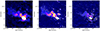 |
Fig. 1. Radio maps of A1213 at different frequencies. Left: 54 MHz LOFAR image of A1213 produced with briggs −0.3. The rms noise is ∼3 mJy beam−1, and white contours are [−3, 3, 6, 12, 24...] × rms. The beam is 22″ × 18″. Central: 144 MHz LOFAR image of A1213 produced with briggs −0.3. The rms noise is ∼100 μJy beam−1, and white contours are [−3, 3, 6, 12, 24...] × rms. The beam is 8″ × 5″. Right: 380 MHz uGMRT image of A1213 produced with briggs −0.3. The rms noise is ∼60 μJy beam−1, and white contours are [−3, 3, 6, 12, 24...] × rms. The beam is 7″ × 5″. |
2.3. uGMRT observation
uGMRT has observed A1213 on 20 February 2022 for a total integration time of 4 hours in band 3 (central frequency ∼380 MHz), as part of the project 41_093 (ObsID 13963, P.I. V. Mahatma). 3C 147 was used as absolute flux density calibrator, while the data reduction and calibration were carried out using the Source Peeling and Atmospheric Modeling (SPAM) pipeline (Intema et al. 2009, 2017). It corrects for ionospheric effects and removes direction-dependent gain errors by adopting a facet approach, similarly to van Weeren et al. (2016). Finally, data were corrected for the system temperature variations between calibrators and target, and imaging was carried out through WSClean applying different weightings and visibility tapering. Flux density uncertainties are assumed to be 6%, as from literature values for uGMRT band 3 (e.g. Chandra et al. 2004; Bruno et al. 2023).
2.4. XMM-Newton observation
A1213 was observed by XMM-Newton on 12 June 2008 for a total of 20 ks (observation ID 0550270101). We processed the data using the XMMSAS v19.1 package and the X-COP analysis pipeline (Ghirardini et al. 2019). After applying the standard cuts for time intervals affected by background flares, the clean observing time is 15.6 ks for the two MOS detectors and 5.3 ks for the PN detector. Our analysis procedure follows that of B23. From the cleaned event lists, we extracted count maps in the [0.7–1.2] keV band. For a discussion of the global IGrM properties of the system (e.g. hydrostatic mass, luminosity, surface brightness, and density profiles), we refer to B23. In this work, the X-ray map has mainly been used for visualization purposes and for a comparison with the non-thermal emission detected in the radio band.
3. Results
In this section, we summarise the results of the analysis of the 54, 144 and 380 MHz images, as well as the spectral index maps we produced. The synchrotron spectrum of 4C 29.41, given its peculiarity, is discussed in detail in Sect. 4.2.
3.1. A1213 at 54 MHz
In the left panel of Fig. 2, we show the 54 MHz LOFAR image of A1213. The morphology of the tail is very similar to what is observed at higher frequency (see B23 and next sections), with a ∼500 kpc trail of emission extending north-east from the radio galaxy (at least in projection). Multiple peaks are visible along the tail. For this source we measured a flux density of S54 MHz = 4.4 ± 0.4 Jy within 3σ contours7. In contrast, in the north and south of 4C 29.41, we observed elliptical emission with orthogonal orientation with respect to the AGN and the tail, which might suggest a divergent nature. This emission is partially blended with a head-tail radio galaxy north-east of 4C 29.41. Indeed, B23 had already observed this ‘patched’ emission at 144 MHz, although the image was not clear due to calibration artefacts (also see the next section). Our calibration strategy for the 54 MHz observation helped to mitigate this effect, which allows for a clearer detection. The detected emission is therefore real and not the result of bad calibration.
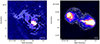 |
Fig. 2. High-resolution LOFAR images of A1213. Left: 144 MHz LOFAR-VLBI image of A1213. The image was produced with a restoring beam of 1.5″ × 1.5″, and with an adapted colorscale to enhance the filamentary emission from the tail. Artefacts due to dynamic range issues are still visible in the image. The rms noise is ∼50 μJy beam−1. Right: 144 MHz LOFAR-VLBI image of 4C 29.41, the central radio galaxy of A1213. The image was produced at a resolution of 0.36″ × 0.19″. The largest angular scale for this data is ∼70″, which prevents the detection of the extended tail in the north-east. Contours are from 2σ to highlight the presence of faint emission, with the σ ∼ 45 μJy beam−1 as the rms noise. |
3.2. A1213 at 144 MHz
In the central panel of Fig. 2, we show the 144 MHz map of A1213. Since a detailed discussion of the 144 MHz radio emission at at a resolution of ∼6″ can be already found in B23, we summarise the main features here. The eastern trail shows a number of emission peaks and a filamentary structure. Moreover, at the eastern tip the radio emission seems to blend with a structure oriented in the north-south direction. This structure is also detected at 54 MHz, although at lower resolution. We confirm that the small-scale emission north of 4C 29.41 is associated to a member galaxy (ID 442 in B23). We also confirm the detection of fragmented emission around the AGN, although that area is contaminated by calibration artefacts. We note that even after our calibration strategy, we did not detect any new radio source in our image compared to B23, while we confirm the detection of all the sources they already found, even at lower and higher frequencies. For the tail (and when excluding 4C 29.41), we measure da flux density of S144 MHz = 1.52 ± 0.15 Jy within 3σ contours.
Thanks to the inclusion of LOFAR international stations, we were able to increase the resolution of the 144 MHz data. In the left panel of Fig. 1, we show the LOFAR-VLBI image at 1.5″ resolution, which confirms the filamentary structure of the tail. It is also worth noting that we clearly detect emission to the north and south of 4C 29.41, which is not visible at the typical 6″ resolution of the HBA image in the central panel of Fig. 2. Nevertheless, calibration artefacts are still visible in the image. In the right panel, we show instead the LOFAR-VLBI image produced by phasing-up the core stations of the LOFAR Dutch array (see Sect. 2.2 for details). While the largest angular scale becomes smaller with this strategy (i.e. ∼70″), implying that we cannot detect the extended tail, we are able to further push the resolution to 0.3″ to better calibrate the data and resolve the central radio galaxy. We observe a typical double-lobed, FRII-like morphology, with two jets (among which only one is visible) departing in the north-east-south-west directions for ∼35 kpc each. At this distance from the AGN core, the interaction with the surrounding IGrM creates two roughly spherical lobes with a ∼40 kpc diameter. While the brightest radio emission is well-confined within the lobes, we did detect fainter structures at 2σ north and south of the east and west lobes, respectively. Finally, at this resolution the AGN does not look connected to the tail.
3.3. A1213 at 380 MHz
In the right panel of Fig. 2, we show the uGMRT map of A1213 at 380 MHz. The tail shows a complex, filamentary structure extending for ∼300 kpc (at 3σ), which is significantly less than what observed at lower frequency. This is just the result of the shape of the synchrotron spectrum, as higher energy electrons lose energy faster. We measure a flux density of S380 MHz = 0.4 ± 0.1 Jy within 3σ contours. We do not detect the north-south structure at the eastern end of the tail, which might also suggest a steep spectrum (see also Sect. 4.3). We highlight the presence of emission north and south to 4C 29.41 even at this frequency but, similarly to the HBA data, dynamic range issues affect the images and produce patches and negatives, preventing us from observing its real morphology.
3.4. Spectral index maps
We have produced spectral index maps between 54, 144 and 380 MHz as follows. First, maps at all frequencies were produced by applying the same visibility cut of 80 λ–14 kλ and Briggs −0.38. This is important in the comparison of images obtained with a different sensitivity to a diffuse low brightness emission, as the two instruments (LOFAR and uGMRT) have different uv-coverages. The spectral index map was then generated by calculating α and Δα in each pixel. Additional details can be found in Appendix A.
3.4.1. LOFAR spectral index map between 54 and 144 MHz
The spectral index map between 54 and 144 MHz is shown in the left panel of Fig. 3, while the spectral index error map can be found in Appendix A9. It has been produced at the smallest common beam (30″ × 25″), at which all the sources of interest are clearly visible.
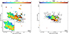 |
Fig. 3. Spectral index maps of A1213. Left: Spectral index map between 54 and 144 MHz (beam 30″ × 25″). Upper limits are represented with downwards arrows. Only emission above 3σ is visible. Overlaid in black are 54 MHz contours. The bottom-left panel is a zoom on the eastern part of the tail. Right: Spectral index map between 144 and 380 MHz (beam 24″ × 19″). Only emission above 3σ is visible. Overlaid in black are 54 MHz contours. In both images, the emission to the north and south of 4C 29.41 is affected by calibration artefacts at 144 and 380 MHz and has been masked. |
We find that for 4C 29.4110 the spectral index is ∼−0.8, consistent with what usually detected in active radio galaxies (Zajaček et al. 2019). The spectral index then steepens moving eastwards and we detect what seems to be a sharp break in the gradient in a small region in between 4C 29.41 and the tail, with steep values of α ∼ −2.3. Interestingly, the southern part of the tail steepens down to α ∼ −1.2 towards east, settling around this value. On the other hand, in the northern-most part, there is a further steepening from ∼−2 down to a minimum value of ∼−3.1. Finally, the eastern edge of the tail shows steep spectral indices with mean value α ∼ −2, with the exception of a thin filament oriented in the north-south direction which shows α ∼ −1.2. This corresponds to the structure previously detected at 144 MHz.
3.4.2. LOFAR-uGMRT spectral index map between 144 and 380 MHz
In the right panel of Fig. 3, we show the spectral index map between 144 and 380 MHz. This has been produced with the same method described for the LOFAR spectral index map, along with a visibility cut of 80 λ–14 kλ. We masked the extended emission north and south to 4C 29.41, since it is affected by dynamic range issues at both frequencies.
As expected, there is less spectral index information at higher frequencies due to the non-detection of steep-spectrum emission. Nevertheless, the spectral index trend is very similar to what is observed at lower frequency. The extended emission east of 4C 29.41 shows values that steepen from ∼−0.7 down to minimum values of ∼−2 at the eastern tip. However, at this higher frequency and distance from the AGN core (∼100 kpc) the width of the tail looks smaller, and it is harder to detect any kind of gradient on the north-south direction, as instead observed with LOFAR, although the northern-most region shows α ∼ −1.4. A significant gradient is instead detected on the west-east axis, namely, moving from the AGN to the tip of the tail, with the spectral index gradually steepening, similarly to what is observed at lower frequencies.
The spectral index of 4C 29.41 is consistent with what observed with LOFAR HBA and LBA. We note that we still detect (even at this frequency) a very small region in-between the AGN and the tail, where there is a break in the spectral index gradient, with values that suddenly steepen down to α ∼ −2. This region is as wide as the restoring beam with which the map was produced.
Finally, we note that the region of the tip of the tail, where the north-south filament is clearly detected at 144 MHz and shows  , is masked with our 3σ threshold. In fact, this structure is only barely detectable at 380 MHz.
4. Discussion
In Fig. 4, we show the radio emission, as observed by LOFAR at 144 MHz, overlaid on the SDSS g-band image. We have labelled relevant features, such as the central AGN, the tail, the eastern edge, and the head-tail radio galaxy, which will be discussed in this section.
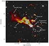 |
Fig. 4. Radio emission from LOFAR at 144 MHz (red) overlaid on the optical image of A1213 from SDSS (g-band). Relevant features that we discuss in this work have been labelled. |
4.1. Origin of the tail
To better visualise and investigate the interplay between thermal and non-thermal emission, in the left panel of Fig. 5, we show the LOFAR 54 MHz 3σ contours overlaid on the adaptively smoothed XMM-Newton map between 0.7 and 1.2 keV. The right panel shows a zoom on 4C 29.41, where we have overlaid 144 MHz contours at 0.3″ resolution. As already reported in B23, the IGrM distribution is not typical of a cool-core system, where the morphology is usually roughly spherical and regular, with a clear core. Instead, we observe an elongated morphology and multiple emission peaks, with only few of them being associated with AGN counterparts. The thermal emission is stretched on the NE-SW direction. While there is no clear X-ray core, the X-ray centroid of the group as identified in B23 lies ∼30 kpc west to 4C 29.41. The map apparently shows knotted X-ray emission surrounded by a lower surface brightness area. This is the result of the relatively short exposure time (i.e. low photon count), combined with the smoothing we applied to enhance the thermal emission. For further details, we refer to B23.
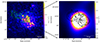 |
Fig. 5. X-ray map of A1213 with overlaid radio contours. Left: LOFAR 54 MHz contours (green) overlaid on the XMM-Newton map in the energy range 0.7−1.2 keV. R200 is ∼1140 kpc, which lies outside of our field of view. Right: Zoom on 4C 29.41 contours as detected at 144 MHz from the 0.3″ resolution image, overlaid on the same XMM-Newton map shown on the left panel. |
The radio emission from the tail develops eastwards from 4C 29.41 for a total extent of ∼500 kpc and apparently shows no clear interplay or spatial correspondence with features observed in the hot gas. The emission around 4C 29.41 seems instead to be distributed following the major axis of the roughly elliptical gas distribution. This is in line with the findings reported in B23 and might suggests a sub-cluster merger in the NE-SW direction. Despite the presence of multiple X-ray peaks in the south-west part of the system, we detected no associated radio emission, either compact or extended, even though the morphology of the thermal emission closely resembles that observed in the north-east region, where non-thermal emission is present.
Previous studies on this system (e.g. Giovannini et al. 2009) first classified the tail as a radio halo. However, as also stated in B23, if this was the case it would be really peculiar, as it is off-centred and elongated with respect to the X-ray emission. Furthermore, it stands out from the X-ray luminosity-radio power correlation (Giovannini et al. 2009), usually observed for radio halos (Feretti et al. 2012; Cassano et al. 2013; Cuciti et al. 2021). Hoang et al. (2022) proposed instead that this emission could be the extended tail of the central radio galaxy. In this scenario, the tail could have reached its current extent thanks to the low IGrM density in that direction. They also suggest that the eastern edge could have been generated by merger shocks interacting with the tail. While this interpretation sounds reasonable, given the spectral index map in Fig. 3, B23 attributes the origin of the tail to a radio relic; namely, the result of a shock that re-accelerated electrons in this region following first-order Fermi processes. They support this hypothesis through a spectral index map between a VLA 1.4 GHz observation11 and the same LoTSS observation from which our data was derived. This map shows a gradient in the north-south direction, with the spectral index steepening from north to south, which would be evidence of a shock propagating in the same direction.
In both our spectral index maps (54−144 MHz and 144−380 MHz), we did indeed detect hints of a gradient in the south-north direction, which can be noted from the zoom on the left panel of Fig. 3. In this region, the spectral index is flatter in the southern part of the tail, and it steepens moving north. This is the opposite of what is seen for B23, where a flatter spectrum is observed in the northern region, which steepens moving south. Our higher-resolution spectral index and total intensity maps clearly show that the brightest emission of the tail is concentrated on the southern region, where the spectral index is flatter. The less energetic electrons in the north are more likely the simple result of interaction with the surrounding medium and ageing due to radiative losses, rather than the consequence of shock re-acceleration, as instead suggested in B23. The distribution of the thermal gas strongly disagrees with the hypothesis of a radio relic, as its orientation is different from what we would expect from the X-ray morphology, which is stretched along the NE-SW axis: a shock would eventually re-accelerate electrons in a direction that would be almost perpendicular to that of the detected radio emission.
The 144 MHz 0.3″ map shows that the current outburst of 4C 29.41 does not hint at any kind of physical connection with the tail. The LOFAR spectral index map shows hints of a spatial break between the AGN and the tail, which are separated by a small (∼20 kpc width) region with very steep spectral index (α ∼ −2.3). It is therefore likely that we are looking at two different sources, and that the tail did not directly develop from the central radio galaxy or at least it does not originate from its current outburst. We suggest two possible scenarios for its origin.
4.1.1. Non-thermal contribution from group members
A first, possible explanation is that member galaxies near the position of 4C 29.41 could have played a role for the formation of the tail. Indeed, we have inspected the Data Release 10 of the DESI Legacy Survey (Dey et al. 2019) at the position of A1213 and we found that there is a number of group member galaxies which could have possibly contributed to the process. In the left panel of Fig. 6, we show the DESI DR10 image with overlaid radio contours, including LOFAR-VLBI. The redshifts come from spectra of SDSS DR16 (Ahumada et al. 2020). An example is the source on the north-west with z = 0.047 (labelled #1 in the figure), which (from SDSS) is an elliptical galaxy whose radio emission is visible even from 144 MHz high-resolution images (e.g. central panel of Fig. 2). If we push the HBA resolution (see right panel of Fig. 6), it is clearly visible that this source hosts an head-tail radio galaxy (as already discussed above) that in the region of the radio core, looks physically disconnected from the extended emission on the east of the group. There are still hints of plasma mixing with the tail in the eastern lobe, as also visible from the right panel of Fig. 6. Nevertheless, from the current data it seems unlikely that galaxy #1 constitutes the major factor for the formation of the tail. Another contribution could have possibly come from an elliptical galaxy at z = 0.05 (labelled #2 in the figure), which lies ∼20 kpc (in projection) south from 4C 29.41. This source was already identified as a companion galaxy to 4C 29.41 in B23. Our high-resolution image at 144 MHz shows that this galaxy does not exhibit radio emission on the same scale of 4C 29.41. Furthermore, the SDSS spectrum does not show any hint of the typical AGN emission lines, suggesting that the galaxy is not currently active, although it might have been in the past. Finally, it is worth noting that the source at z = 0.049 west to 4C 29.41 (labelled #3 in the figure), identified as the BGG in B23, does not appear to be connected with the tail, at least at low frequency. In summary, while radio emission from these galaxies (when present) could have possibly contributed to the formation of the tail, they hardly played the dominant role.
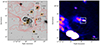 |
Fig. 6. Zoom-in images on member galaxies of A1213. Left: DR10 DESI Legacy Survey optical image of the inner region of A1213. Overlaid are the 54 MHz contours at ∼12″ resolution (red) and the 144 MHz contours at ∼0.3″ resolution (black). Yellow circles denote members of A1213 that could be related to the elongated tail, with their corresponding redshift from SDSS. Right: 144 MHz image at ∼6″ resolution zoomed onto the elliptical galaxy on the north-west region of A1213. The optical galaxy is surrounded by a white square. |
4.1.2. Group weather and galaxy motions
A second possible explanation is that the tail originated from a past AGN activity of 4C 29.41, while the double-lobe emission represents the current outburst. This idea is supported by our spectral index maps, which show a sudden break in the gradient between 4C 29.41 and the tail, as well as by the merger’s orientation along the NE-SW axis, as suggested by the X-ray morphology (see B23). In this scenario, the active radio galaxy might be moving along this axis, leaving behind a trail of older electrons injected during a previous outburst. These features in A1213 closely resemble those observed in another dumb-bell galaxy, NGC 326, by Hardcastle et al. (2019). In that system, the western wing appears confined, while the eastern one has a tail-like extension with a filamentary structure and a sharp edge, similar to what we see in A1213. They propose that large-scale hydrodynamical processes, possibly combined with black hole interaction, could explain the observed morphology. In A1213, an initial outburst of 4C 29.41 could have released a population of seed electrons, while the galaxy continued moving southwest along the line of sight (B23). Following this first event, a second, more recent outburst likely produced the double-lobed structure resolved at 0.3″ resolution. If this is the case, the tail might consists of old, re-energised AGN plasma, akin to radio phoenixes sometimes found in disturbed galaxy clusters (e.g. Enßlin & Brüggen 2002; de Gasperin et al. 2015; Mandal et al. 2019; Pasini et al. 2022a). The observed filaments may trace magnetic field enhancements possibly caused by the ongoing merger. Additionally, the orientation of the eastern edge suggests thermal pressure is preventing further expansion of the tail, bending the structure. In conclusion, the current environment of A1213 likely results from a combination of multiple AGN outbursts and group dynamics, with mergers and gas motions shaping the non-thermal emission.
While it is not trivial to conclusively prove this scenario, we can perform a number of tests to check and confirm that the tail is not physically related to the current outburst of 4C 29.41. First of all, to eventually trace gradients in the spectral shape of the electron energy distribution between lower and higher frequency, we produced a spectral curvature map (SC map). Similarly to the one from Rajpurohit et al. (2021), for instance, we started by deriving the curvature in each pixel as:
 (1)
(1)
This derivation was applied to spectral index maps between 54−144 MHz and 144−380 MHz by convolving them at the smallest common beam where the extended emission is clearly visible; namely, with ∼20″ × 20″ resolution. The SC map is shown in Fig. 7.
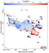 |
Fig. 7. Spectral curvature (SC) map between 54−144 MHz and 144−380 MHz at ∼20″ resolution. A negative value implies a convex spectral shape. |
The ‘edges’ of the radio emission are affected by large errors from the spectral index maps. For this reason, we have not commented on the significantly higher (or lower) SC values in the regions surrounding the black contours. In the region of 4C 29.41, the SC values are mostly positive or close to 0, implying that the spectrum is not significantly steepening from low to high frequency, as expected from a situation where the AGN outburst is most likely still occurring (or has occurred recently). On the other hand, the tail shows hints of a negative curvature, which becomes more significant as we move eastwards; namely, the high-frequency spectral index is becoming steeper and steeper, compared to the low-frequency index. Most importantly, we also note a rather sharp break in the SC distribution between the tail and the region of 4C 29.41, as the SC suddenly decreases from ∼0.5 to ∼−0.3. This supports the scenario where the double-lobed structure is physically disconnected from the elongated emission, as we are detecting two different outbursts that happened on different timescales.
Another hint that the two emissions are currently unrelated, and in fact might come from different outbursts of the same central engine source, comes from the synchrotron ageing models. In the absence of particle re-acceleration, the electron population is expected to age due to radiative (synchrotron and Inverse Compton, IC) and adiabatic losses. In this ‘pure-aging’ scenario, if the tail originated from the current outburst of 4C 29.41, we should observe a spatial evolution of the spectral index along the extended emission moving eastwards from the AGN. In more detail, the spectral index should be flatter (α ∼ −0.6) in the injection point and then gradually become steeper as we move along the tail. To test this hypothesis, we have sampled the flux density starting from the injection point of the electrons, which we assumed to be spatially coincident with the AGN core in the case where the tail directly develops from 4C 29.41, then moving along the extended emission (as shown in the left panel of Fig. 8). Each sampling region is as large as the smallest common beam (23″ × 23″) of 54, 144 and 380 MHz images, which were suitably produced with a matched uv-cut as already discussed in Sect. 3.4. For each region, we estimate the spectral index between 54 and 144 MHz and between 144 and 380 MHz. The spectral index distribution is then fitted through a Jaffe-Perola (JP) model (Jaffe & Perola 1973), for which we assumed that the break frequency is the same at a given distance. In this model, as we assumed an injection index α = −0.8 from our spectral index map, the ageing of the electrons population is dependent only upon the magnetic field strength and the projected velocity of the host galaxy through the cluster environment; namely, the IGrM. To maximise the lifetime of the electron population (so that we get is an upper limit on the radiative age), we have assumed a minimum loss magnetic field of  , with BCMB = 3.2 × (1 + z)2 μG being the magnetic field strength of the cosmic microwave background (CMB) at a redshift of z. We get Bmin = 2.03 μG, which is consistent with the estimate of 2−3 μG reported in B23. At this point, the only free parameter is the galaxy velocity (see also Edler et al. 2022). The result is shown in the right panel of Fig. 8.
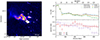 |
Fig. 8. Results of the JP fit on A1213. Left: Regions from which the spectral index was sampled and fit with a JP model, overlaid on the 144 MHz map. Right: Flux density at different frequencies for each region (top) and the corresponding spectral index and the fit with a JP model (bottom). |
The synchrotron ageing model clearly fails to reproduce the observed behaviour of the spectral index. We obtain in fact a galaxy velocity of ∼2785 km/s, and a reduced χ2-squared of χ2/d.o.f. = 1641 (where d.o.f. are the degrees of freedom), which is an obvious indicator that the model is not providing a correct description of the data. The flux density distribution along the extended emission follows indeed a non-trivial behaviour, exhibiting a sharp and sudden decrease as soon as we move out of the brightest region, which we would not expect if the tail directly originated from it. The spectral index distribution is also complex: the current outburst shows a convex spectrum (as also found in Fig. 7), with the higher-frequency spectral index being flatter than the low-frequency one12. On the other hand, moving along the tail we find a more typical trend, with a gradual steepening. However, we also note that the outermost part of the tail (∼300 kpc onwards from the AGN core) shows a rather constant spectral index at low-frequency, while at a higher frequency, it exhibits the typical steepening of the synchrotron spectrum. It reaches a plateau at greater distance from the (supposedly) injection point. While similar cases of tails mildly re-energised by turbulence have already been found (de Gasperin et al. 2017), the complex spectral index distribution observed for this source prevents us from drawing further conclusions.
Nevertheless, it is clear that a simple pure-aging model along the AGN and tail (assuming that the latter originated from the same outburst that is currently supporting the former) is not able to reliably describe the spectral shape. The most obvious explanation for the observed distribution is that we are indeed looking at two different sources.
4.2. The synchrotron spectrum of 4C 29.41
We have measured the integrated flux density within 3σ contours of 4C 29.41 at all our three frequencies13 to study its synchrotron spectrum in more detail. These results are summarised in Table 1. If we estimate the spectral index using these values, we find  and
and  , which confirms the positive curvature already found in Fig. 7. Furthermore, we also retrieved the 1.4 GHz image from the FIRST survey (Faint Images of the Radio Sky at Twenty-Centimeters, Becker et al. 1994) and estimated the high-frequency spectral index between 380 MHz and 1.4 GHz, α = −0.53 ± 0.09, which further confirms the convex shape. Given the morphology and extension of the radio galaxy, a flattening of the spectrum moving to higher frequency is somehow unexpected.
Integrated flux density and spectral indices of 4C 29.41 at 54, 144 and 380 MHz.
First, we checked the flux scale of our images, either by using available surveys at close frequencies (e.g. the TIFR GMRT Sky Survey at 150 MHz, TGSS, Intema et al. 2017) or by re-scaling the flux density of point sources in the field assuming a typical spectral index of α = −0.8. We confirmed that our data do not show any obvious flux scale mismatch exceeding the expected systematic uncertainties (see Sect. 2).
We then investigated whether the observed spectrum could be the result of the combination of two components: one steeper and one flatter. The companion galaxy of 4C 29.41 is slightly offset from the radio galaxy; furthermore, if we separately measure the spectral index of the two lobes, we find that the two spectra are consistent with each other and the observed flattening at higher frequency exists for both lobes. We have then considered the hypothesis that extended emission from the tail might be contaminating the region of the radio galaxy (i.e. adding spurious flux). In this scenario, the lower frequencies should be more affected by this issue, because of the spectral shape of the tail. We should be able to remove most of the extended sources contribution by applying a specific uv-cut when cleaning, so that sources above a certain LLS are not imaged. Since the LLS of the radio galaxy is ∼2′, we have produced images at 54, 144, and 380 MHz by cutting all visibilities below 1.6 kλ, and we again measured the integrated flux density. In this way, only the radio galaxy is imaged and we end up losing the larger scale emission. Results are listed in Table 1 and shown in Fig. 9.
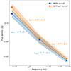 |
Fig. 9. Synchrotron spectrum of 4C 29.41 between 54 and 380 MHz. The orange curve shows the case where no uv-cut was applied while imaging, thus including the contribution of extended emission, that increases the flux density especially at lower frequency. The blue curve shows instead the case with a minimum uv-cut of 1.6 kλ, which roughly corresponds to 2′ (i.e. the larger scale emission is not present). |
The 54 MHz data is particularly affected by this problem, since the extended emission primarily radiates at lower frequencies and can clearly be detected, significantly contaminating the flux density measurement of the radio galaxy. On the other hand, we find a less dominant effect at 144 and 380 MHz. By removing the contribution of the large-scale emission from the tail, the synchrotron spectrum of the radio galaxy in the range 54−300 MHz is consistent with a power-law with α ∼ −0.7 within uncertainties, which is typical for this kind of sources. Finally, it is worth mentioning that the flattening observed when accounting for the FIRST measurement at 1.4 GHz is instead probably driven by the core, which starts to dominate the total source flux density at these higher frequencies.
4.3. The eastern edge: Tip of the tail or radio relic
The north-south oriented edge detected at 144 MHz in the eastern part of the tail shows the typical morphology of a radio relic. Its orientation with respect to the IGrM (and, thus, to the merger axis) is also in agreement with this hypothesis. Indeed, Hoang et al. (2022) first suggested the presence of a shock in the east-west direction, which could have generated the source. However, the region is too thin and our resolution not high enough to detect any kind of spectral index gradient in the LOFAR map. We have therefore estimated the integrated flux density within 3σ contours at 54 and 144 MHz, finding 513 ± 51 mJy and 126 ± 13 mJy, respectively, which yields α = −1.4 ± 0.15. While this is obviously in agreement with the spectral index map in the left panel of Fig. 3, it is only marginally consistent with the usual integrated values (∼ − 1.2) observed in radio relics (see e.g. van Weeren et al. 2019).
This structure is not detected by uGMRT at 380 MHz. It is only by performing a significant tapering of the visibilities we start to observe faint hints of the source, although image negatives affect this region. Therefore, it is not possible to accurately estimate the integrated flux density at this frequency. Nevertheless, we can assume that the spectral index is the same than what found at lower frequency and predict the expected flux density value: this yields an integrated flux density of ∼32 mJy at 380 MHz. Given the rms-noise of the uGMRT image14, we should clearly be able to detect it if this was the case, which suggests that the real value is lower; therefore, the spectral index is steeper. Indeed, if we use the same 3σ contours exploited at 144 MHz and the rms noise mentioned above, we get an upper limit on the integrated flux density of ∼25 mJy, which consequently leads to an upper limit on the spectral index  . This steepening is not commonly observed in radio relics. Furthermore, no X-ray discontinuity was identified in B23, which could hint at the presence of a shock propagating through this region. We can conclude that this source is just the final part of the tail. The different orientation is likely due to the interaction with the surrounding IGrM, which has bent the structure. This also explain the steeper spectral index observed in Fig. 3.
4.4. Considering whether A1213 could host diffuse radio emission
B23 reports the presence of fragmented radio emission close to the group X-ray centroid, around the BGG, which they attribute to a candidate radio halo, although their data did not allow to investigate further. Their 144 image is affected by calibration artefacts in this region, most likely because of the brightness of 4C 29.41. On the other hand, our calibration strategy significantly improved this aspect. Once artefacts are removed, the BGG shows a rather compact radio emission, with no hints of diffuse structures.
However, we note that the left panel of Fig. 2 shows the presence of roundish (although slightly elongated on the north-south axis) diffuse radio emission around 4C 29.41, which is visible even at high resolution and especially from the source-subtracted map shown in the left panel of Fig. 10. The same emission is also detected in the LOFAR-VLBI image in the left panel of Fig. 1. While it is possible that it could be part of the inner side of the tail, the different morphology might also hint at a different origin. Unfortunately, we had to mask this region when producing the spectral index maps in Fig. 3 because of the presence of calibration artefacts and negatives in the 144 and 380 MHz image. Therefore, it is currently not possible to constrain the synchrotron spectrum of the diffuse emission, nor to put upper limits. Nevertheless, we can try to speculate on its nature based on the currently available data.
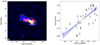 |
Fig. 10. Results of the point-to-point analysis on the central region of A1213. Left: Source-subtracted map of A1213 at 54 MHz, where all sources with LLS < 250 kpc have been removed. It is not possible to remove the whole emission from 4C 29.41, which blends together with the tail and with the roundish emission in the western region. The red grid shows the region of interest of the point-to-point analysis, while the green contours encircle the region where 4C 29.41 is located. Right: Result of the point-to-point analysis between the X-ray and the LOFAR LBA source-subtracted image of A1213. The surface brightness is estimated as the sum of every pixel in each square of the grid, divided by its area. The blue line shows the best fit in the form Y = kX + A, where k = 0.25 ± 0.04 and A = −2.36 ± 0.26. |
A possibility is that this emission first originated from 4C 29.41 and then got trapped in the central region of the group, evolving to a low-surface-brightness source that might resemble clusters’ mini-halos (van Weeren et al. 2019). In this scenario, seed fossil electrons are provided by the central AGN. It is also possible that other active group members might have contributed in the past, although SDSS spectra of galaxies in Fig. 6 do not currently show any emission line typical of AGN.
A well-known physical correlation, which directly arises from the connection between mini-halos and ICM motions, exists between their radio power and the host cluster X-ray luminosity (see e.g. Biava et al. 2021; Riseley et al. 2022). Therefore, we exploited PT-REX (Ignesti 2022) to trace the radio and X-ray surface brightness of the diffuse emission through a point-to-point analysis (Govoni et al. 2001; Rajpurohit et al. 2021). To avoid the calibration artefacts and contamination from 4C 29.41 as much as possible, the algorithm was applied to the 54 MHz source-subtracted data, which is the cleanest in this region; leftover spurious emission in the centre of the AGN and in the region of the head-tail in the north was masked. The algorithm designs a grid above the region of interest (shown in the left panel of Fig. 10) and samples the surface brightness in each square of the grid from the radio and X-ray images. The grid was carefully selected to avoid the region of 4C 29.41 and the southern part of its radio emission; namely, the proximity of the location of the companion galaxy before the source subtraction. We put instead the focus on the northern region, where the contamination from the AGN is expected to be less prominent. The result is shown in the right panel of Fig. 10.
The surface brightness values show a correlation, albeit scattered. The best fit, computed in the form of Y = kX + A, shows k = 0.25 ± 0.04 and A = −2.36 ± 0.26; namely, this is a sub-linear correlation that is usually typical of giant halos, rather than mini-halos. The Pearson and Spearman indices are both ∼0.72, which translates into a very low p-value of ∼10−5. While this might indicate a real correlation, it is also worth noting that the analysis had to be restricted to a very small region because of possible AGN contamination. For the same reason, we are not sampling the southern part of the emission. Therefore, it is currently hard to derive strong conclusions about its origin. While the hypothesis of a mini-halo in a galaxy group is tempting, especially considering the observed physical and spatial correlation with the thermal gas, it is not possible to exclude the possibility that this emission might just constitute the inner part of the tail, or that it might just be plasma being transported by the ‘weather’ of the IGrM, similarly to, for example, NGC 507 (Brienza et al. 2022). Finally, it is also worth noting that mini-halos are usually observed in systems hosting cool cores (e.g. Govoni et al. 2009; Biava et al. 2021), whereas A1213 shows multiple X-ray peaks and no clear core.
5. Conclusions
In this work, we investigate the low-frequency radio emission in the galaxy group A1213 by exploiting proprietary LOFAR 54 MHz and uGMRT 380 MHz observations. As found in previous studies (e.g. B23), this system is a galaxy group with ∼143 galaxy members and a disturbed and elongated X-ray morphology. We have complemented our data with reprocessed LOFAR 144 MHz observations at both 6″ and 0.3″ resolution from LoTSS, along with an archival XMM-Newton observation. Our results can be summarised as follows:
-
A1213 exhibits complex radio emission at low frequency. One of the brightest group members, 4C 29.41, which is classified as a dumb-bell galaxy (i.e. it has two optical nuclei), hosts a bright FRII radio galaxy with two symmetric lobes. Only the western jet is detected from our 144 MHz 0.3″ images, likely because of relativistic boosting. From the same region of 4C 29.41, a striking ∼500 kpc-long trail of emission extends eastwards.
-
The trail is detected at all our three frequencies and shows multiple emission peaks along its length. The spectral index maps reveal that the spectral index steepens from the AGN core down to the edge of the emission, reaching α ∼ −2.5 in the outer side and showing a sudden break between the region of 4C 29.41 and the tail. A roundish spot of flatter emission is detected on the tip. Our evidence support the hypothesis that the source is a radio tail, which is directly extended from the region of 4C 29.41, rather than a radio relic, as previously suggested in recent studies.
-
We produced a spectral curvature (SC) map and studied the spectral index distribution along the tail by fitting it with a standard JP synchrotron model. Together with the well-confined morphology of the FRII radio galaxy, this evidence suggests that the tail did not directly originate from the current outburst of 4C 29.41, but it is likely the result of a past activity of its central engine, which expanded along a less dense region of the IGrM. In a later phase, the galaxy kept moving along the line of sight, producing the current FRII morphology in a more recent outburst. On the other hand, the old plasma was left behind and started to shine again due to re-acceleration mechanisms, as suggested from the spectral index plateau observed in Fig. 8. The current state of A1213 might therefore be the result of a combination of galaxy motions, re-started AGN activity and group weather.
-
The thermal emission from the IGrM shows multiple peaks of emission and an elongated south-west–north-east morphology, with no obvious core. The X-ray centroid was previously identified in B23 to be ∼30 kpc west of 4C 29.41. The non-thermal emission is somehow present only in the north–east region of the hot IGrM, while in the south-west part of the group, no radio source is detected at all frequencies.
-
In the eastern part of the tail we observe a thin (∼30 kpc) filament oriented in the north-south direction. This structure is not detected at 380 MHz unless by performing a significant tapering of the visibilities. Its location and morphology might be indicative of a radio relic. We find an integrated spectral index α ∼ −1.4 between 54 and 144 MHz. It is shown to significantly steepen at higher frequencies, which is not typical of relics. This fact, together with the physical connection observed with the tail, likely excludes the hypothesis of a diffuse source. This points instead to an interaction of the terminal part of the tail with the surrounding IGrM.
-
We investigated the nature of the emission around 4C 29.41, which was already tentatively detected in B23 with 144 MHz data. Candidate diffuse emission is clearly observed at 54 MHz and 144 MHz (although only from 1.5″ resolution images) thanks to our calibration strategy. The point-to-point analysis between the radio and the X-ray surface brightness seems to hint at a possible physical connection between the thermal gas and non-thermal plasma. In this scenario, a plausible hypothesis would be that of a mini-halo, whose seed electrons might have been injected by the activity 4C 29.41 itself. Nevertheless, AGN contamination, even after source subtraction, prevents us from performing a thorough spectral analysis, which would help to assess the true nature of this emission. We cannot currently exclude the hypothesis that this source could actually be just the inner part of the tail or plasma transported by the IGrM.
A1213 is only the first galaxy group among the X-GAP sample that we have investigated at low radio frequencies, thanks to the available wealth of data. However, it has already revealed a plethora of interesting features. Our study confirms once more that galaxy groups are not merely a scaled-down version of galaxy clusters and that it is essential to focus on the interplay between thermal and non-thermal emission even in this lower-mass regime. Combining low-frequency radio data with X-ray observations can provide crucial insights into the role of AGN in the evolution of galaxy groups and help to assess the outburst history that has shaped their current state.
Sν ∝ να, with Sν being the flux density at frequency ν and α being the spectral index.
The exposure time per system differs.
R500 ∼ 650 kpc.
In C and C/D configuration.
Excluding the central AGN.
Chosen to emphasize the extended emission.
Median uncertainties are Δα ∼ 0.15.
Radio galaxy only, excluding the tail.
Taken on March 6th, 2008 (C configuration) and June 2nd, 2008 (C/D configuration).
Although errors remain quite large.
At the same resolution.
∼0.3 mJy beam−1 if we taper at 30″.
Acknowledgments
We thank the referee for useful comments and suggestions. The LOFAR LBA data utilized in this study was awarded as a prize for winning the 2022 LOFAR Boat Race held in Cologne. FdG acknowledges the support of the ERC Consolidator Grant ULU 101086378. DH is supported by the Deutsche Forschungsgemeinschaft (DFG, German Research Foundation) under research unit FOR 5195: “Relativistic Jets in Active Galaxies”). RS acknowledges the support of the Department of Atomic Energy, Government of India, under project no. 12-R&D-TFR-5.02-0700. The research leading to these results has received funding from the European Union’s Horizon 2020 research and innovation programme under grant agreement No 101004719 [ORP]. The Low Frequency Array, designed and constructed by ASTRON, has facilities in several countries, that are owned by various parties (each with their own funding sources), and that are collectively operated by the International LOFAR Telescope (ILT) foundation under a joint scientific policy. We thank the staff of the GMRT that made these observations possible. GMRT is run by the National Centre for Radio Astrophysics of the Tata Institute of Fundamental Research. This research has made use of NASA’s Astrophysics Data System. This research has made use of SAOImage DS9, developed by Smithsonian Astrophysical Observatory.
References
- Abell, G. O., Corwin, H. G., & Olowin, R. P. 1989, ApJS, 70, 1 [Google Scholar]
- Ackermann, M., Ajello, M., Atwood, W. B., et al. 2010, Phys. Rev. D, 82, 092004 [Google Scholar]
- Ahumada, R., Allende Prieto, C., Almeida, A., et al. 2020, ApJS, 249, 3 [NASA ADS] [CrossRef] [Google Scholar]
- Becker, R. H., White, R. L., & Helfand, D. J. 1994, ASP Conf. Ser., 61, 165 [NASA ADS] [Google Scholar]
- Biava, N., de Gasperin, F., Bonafede, A., et al. 2021, MNRAS, 508, 3995 [NASA ADS] [CrossRef] [Google Scholar]
- Bîrzan, L., Rafferty, D. A., McNamara, B. R., Wise, M. W., & Nulsen, P. E. J. 2004, ApJ, 607, 800 [Google Scholar]
- Bonafede, A., Brüggen, M., van Weeren, R., et al. 2012, MNRAS, 426, 40 [Google Scholar]
- Boschin, W., Girardi, M., Grandi, S. D., et al. 2023, A&A, 672, A199 [NASA ADS] [CrossRef] [EDP Sciences] [Google Scholar]
- Brienza, M., Lovisari, L., Rajpurohit, K., et al. 2022, A&A, 661, A92 [NASA ADS] [CrossRef] [EDP Sciences] [Google Scholar]
- Brienza, M., Gilli, R., Prandoni, I., et al. 2023, A&A, 672, A179 [NASA ADS] [CrossRef] [EDP Sciences] [Google Scholar]
- Brüggen, M., & Kaiser, C. R. 2002, Nature, 418, 301 [CrossRef] [Google Scholar]
- Brunetti, G., & Lazarian, A. 2007, MNRAS, 378, 245 [Google Scholar]
- Brunetti, G., & Lazarian, A. 2011, MNRAS, 410, 127 [Google Scholar]
- Brunetti, G., Setti, G., Feretti, L., & Giovannini, G. 2001, MNRAS, 320, 365 [Google Scholar]
- Brunetti, G., Giacintucci, S., Cassano, R., et al. 2008, Nature, 455, 944 [Google Scholar]
- Bruno, L., Rajpurohit, K., Brunetti, G., et al. 2021, A&A, 650, A44 [NASA ADS] [CrossRef] [EDP Sciences] [Google Scholar]
- Bruno, L., Botteon, A., Shimwell, T., et al. 2023, A&A, 678, A133 [NASA ADS] [CrossRef] [EDP Sciences] [Google Scholar]
- Cassano, R., & Brunetti, G. 2005, MNRAS, 357, 1313 [Google Scholar]
- Cassano, R., Ettori, S., Brunetti, G., et al. 2013, ApJ, 777, 141 [Google Scholar]
- Chandra, P., Ray, A., & Bhatnagar, S. 2004, ApJ, 612, 974 [Google Scholar]
- Clark, N. E., Tadhunter, C. N., Morganti, R., et al. 1997, MNRAS, 286, 558 [NASA ADS] [CrossRef] [Google Scholar]
- Cuciti, V., Cassano, R., Brunetti, G., et al. 2021, A&A, 647, A51 [EDP Sciences] [Google Scholar]
- de Gasperin, F., van Weeren, R. J., Brüggen, M., et al. 2014, MNRAS, 444, 3130 [NASA ADS] [CrossRef] [Google Scholar]
- de Gasperin, F., Ogrean, G. A., van Weeren, R. J., et al. 2015, MNRAS, 448, 2197 [NASA ADS] [CrossRef] [Google Scholar]
- de Gasperin, F., Intema, H. T., Shimwell, T. W., et al. 2017, Sci. Adv., 3, e1701634 [Google Scholar]
- de Gasperin, F., Dijkema, T. J., Drabent, A., et al. 2019, A&A, 622, A5 [NASA ADS] [CrossRef] [EDP Sciences] [Google Scholar]
- de Gasperin, F., Williams, W. L., Best, P., et al. 2021, A&A, 648, A104 [NASA ADS] [CrossRef] [EDP Sciences] [Google Scholar]
- de Gasperin, F., Edler, H. W., Williams, W. L., et al. 2023, A&A, 673, A165 [NASA ADS] [CrossRef] [EDP Sciences] [Google Scholar]
- de Jong, J. M. G. H. J., van Weeren, R. J., Sweijen, F., et al. 2024, A&A, 689, A80 [NASA ADS] [CrossRef] [EDP Sciences] [Google Scholar]
- Dey, A., Schlegel, D. J., Lang, D., et al. 2019, AJ, 157, 168 [Google Scholar]
- Di Gennaro, G., van Weeren, R. J., Brunetti, G., et al. 2021, Nat. Astron., 5, 268 [Google Scholar]
- Eckert, D., Gastaldello, F., O’Sullivan, E., et al. 2024, Galaxies, 12, 24 [NASA ADS] [CrossRef] [Google Scholar]
- Edler, H. W., de Gasperin, F., Brunetti, G., et al. 2022, A&A, 666, A3 [NASA ADS] [CrossRef] [EDP Sciences] [Google Scholar]
- Enßlin, T. A., & Brüggen, M. 2002, MNRAS, 331, 1011 [Google Scholar]
- Ettori, S., Gastaldello, F., Gitti, M., et al. 2013, A&A, 555, A93 [NASA ADS] [CrossRef] [EDP Sciences] [Google Scholar]
- Fanti, C., Fanti, R., Feretti, L., et al. 1982, A&A, 105, 200 [NASA ADS] [Google Scholar]
- Feretti, L., Giovannini, G., Govoni, F., & Murgia, M. 2012, A&ARv, 20, 54 [Google Scholar]
- Gastaldello, F., Simionescu, A., Mernier, F., et al. 2021, Universe, 7, 208 [NASA ADS] [CrossRef] [Google Scholar]
- Ghirardini, V., Eckert, D., Ettori, S., et al. 2019, A&A, 621, A41 [NASA ADS] [CrossRef] [EDP Sciences] [Google Scholar]
- Ghisellini, G., & Celotti, A. 2001, A&A, 379, L1 [NASA ADS] [CrossRef] [EDP Sciences] [Google Scholar]
- Giovannini, G., Tordi, M., & Feretti, L. 1999, New Astron., 4, 141 [CrossRef] [Google Scholar]
- Giovannini, G., Bonafede, A., Feretti, L., et al. 2009, A&A, 507, 1257 [NASA ADS] [CrossRef] [EDP Sciences] [Google Scholar]
- Govoni, F., Feretti, L., Giovannini, G., et al. 2001, A&A, 376, 803 [CrossRef] [EDP Sciences] [Google Scholar]
- Govoni, F., Murgia, M., Markevitch, M., et al. 2009, A&A, 499, 371 [NASA ADS] [CrossRef] [EDP Sciences] [Google Scholar]
- Gupta, Y., Ajithkumar, B., Kale, H. S., et al. 2017, Curr. Sci., 113, 707 [NASA ADS] [CrossRef] [Google Scholar]
- Hardcastle, M. J., Croston, J. H., Shimwell, T. W., et al. 2019, MNRAS, 488, 3416 [Google Scholar]
- Hardcastle, M. J., Shimwell, T. W., Tasse, C., et al. 2021, A&A, 648, A10 [EDP Sciences] [Google Scholar]
- Hill, G. J., & Lilly, S. J. 1991, ApJ, 367, 1 [NASA ADS] [CrossRef] [Google Scholar]
- Hoang, D. N., Brüggen, M., Botteon, A., et al. 2022, A&A, 665, A60 [NASA ADS] [CrossRef] [EDP Sciences] [Google Scholar]
- Ignesti, A. 2022, New Astron., 92, 101732 [NASA ADS] [CrossRef] [Google Scholar]
- Intema, H. T., van der Tol, S., Cotton, W. D., et al. 2009, A&A, 501, 1185 [NASA ADS] [CrossRef] [EDP Sciences] [Google Scholar]
- Intema, H. T., Jagannathan, P., Mooley, K. P., & Frail, D. A. 2017, A&A, 598, A78 [NASA ADS] [CrossRef] [EDP Sciences] [Google Scholar]
- Jaffe, W. J., & Perola, G. C. 1973, A&A, 26, 423 [NASA ADS] [Google Scholar]
- Jones, C., & Forman, W. 1999, ApJ, 511, 65 [NASA ADS] [CrossRef] [Google Scholar]
- Kang, H. 2017, J. Korean Astron. Soc., 50, 93 [NASA ADS] [CrossRef] [Google Scholar]
- Kolokythas, K., O’Sullivan, E., Raychaudhury, S., et al. 2018, MNRAS, 481, 1550 [NASA ADS] [Google Scholar]
- Kolokythas, K., O’Sullivan, E., Intema, H., et al. 2019, MNRAS, 489, 2488 [CrossRef] [Google Scholar]
- Kolokythas, K., Vaddi, S., O’Sullivan, E., et al. 2022, MNRAS, 510, 4191 [CrossRef] [Google Scholar]
- Ledlow, M. J., & Owen, F. N. 1995, AJ, 109, 853 [NASA ADS] [CrossRef] [Google Scholar]
- Mandal, S., Intema, H. T., Shimwell, T. W., et al. 2019, A&A, 622, A22 [NASA ADS] [CrossRef] [EDP Sciences] [Google Scholar]
- Marchesini, D., Celotti, A., & Ferrarese, L. 2004, MNRAS, 351, 733 [CrossRef] [Google Scholar]
- McNamara, B. R., & Nulsen, P. E. J. 2012, New J. Phys., 14, 055023 [NASA ADS] [CrossRef] [Google Scholar]
- Morabito, L. K., Jackson, N. J., Mooney, S., et al. 2022, A&A, 658, A1 [NASA ADS] [CrossRef] [EDP Sciences] [Google Scholar]
- Morganti, R., Fogasy, J., Paragi, Z., Oosterloo, T., & Orienti, M. 2013, Science, 341, 1082 [NASA ADS] [CrossRef] [Google Scholar]
- Offringa, A. R., McKinley, B., Hurley-Walker, N., et al. 2014, MNRAS, 444, 606 [Google Scholar]
- Osinga, E., van Weeren, R. J., Brunetti, G., et al. 2024, A&A, 688, A175 [NASA ADS] [CrossRef] [EDP Sciences] [Google Scholar]
- O’Sullivan, E., Ponman, T. J., Kolokythas, K., et al. 2017, MNRAS, 472, 1482 [CrossRef] [Google Scholar]
- O’Sullivan, E., Combes, F., Salomé, P., et al. 2018, A&A, 618, A126 [NASA ADS] [CrossRef] [EDP Sciences] [Google Scholar]
- Pasini, T., Brüggen, M., de Gasperin, F., et al. 2020, MNRAS, 497, 2163 [NASA ADS] [CrossRef] [Google Scholar]
- Pasini, T., Finoguenov, A., Brüggen, M., et al. 2021, MNRAS, 505, 2628 [NASA ADS] [CrossRef] [Google Scholar]
- Pasini, T., Edler, H. W., Brüggen, M., et al. 2022a, A&A, 663, A105 [NASA ADS] [CrossRef] [EDP Sciences] [Google Scholar]
- Pasini, T., Brüggen, M., Hoang, D. N., et al. 2022b, A&A, 661, A13 [NASA ADS] [CrossRef] [EDP Sciences] [Google Scholar]
- Pasini, T., De Gasperin, F., Brüggen, M., et al. 2024, A&A, 689, A218 [NASA ADS] [CrossRef] [EDP Sciences] [Google Scholar]
- Rafferty, D. A., McNamara, B. R., Nulsen, P. E. J., & Wise, M. W. 2006, ApJ, 652, 216 [NASA ADS] [CrossRef] [Google Scholar]
- Rajpurohit, K., Vazza, F., van Weeren, R. J., et al. 2021, A&A, 654, A41 [NASA ADS] [CrossRef] [EDP Sciences] [Google Scholar]
- Rengelink, R. B., Tang, Y., de Bruyn, A. G., et al. 1997, A&AS, 124, 259 [NASA ADS] [CrossRef] [EDP Sciences] [Google Scholar]
- Riseley, C. J., Rajpurohit, K., Loi, F., et al. 2022, MNRAS, 512, 4210 [NASA ADS] [CrossRef] [Google Scholar]
- Shimwell, T. W., Tasse, C., Hardcastle, M. J., et al. 2019, A&A, 622, A1 [NASA ADS] [CrossRef] [EDP Sciences] [Google Scholar]
- Shimwell, T. W., Hardcastle, M. J., Tasse, C., et al. 2022, A&A, 659, A1 [NASA ADS] [CrossRef] [EDP Sciences] [Google Scholar]
- Tasse, C., Hugo, B., Mirmont, M., et al. 2018, A&A, 611, A87 [NASA ADS] [CrossRef] [EDP Sciences] [Google Scholar]
- Tasse, C., Shimwell, T., Hardcastle, M. J., et al. 2021, A&A, 648, A1 [EDP Sciences] [Google Scholar]
- van der Tol, S., Veenboer, B., & Offringa, A. R. 2018, A&A, 616, A27 [NASA ADS] [CrossRef] [EDP Sciences] [Google Scholar]
- van Haarlem, M. P., Wise, M. W., Gunst, A. W., et al. 2013, A&A, 556, A2 [NASA ADS] [CrossRef] [EDP Sciences] [Google Scholar]
- van Weeren, R. J., Röttgering, H. J. A., Brüggen, M., & Hoeft, M. 2010, Science, 330, 347 [Google Scholar]
- van Weeren, R. J., Williams, W. L., Hardcastle, M. J., et al. 2016, ApJS, 223, 2 [Google Scholar]
- van Weeren, R. J., de Gasperin, F., Akamatsu, H., et al. 2019, Space Sci. Rev., 215, 16 [Google Scholar]
- van Weeren, R. J., Shimwell, T. W., Botteon, A., et al. 2021, A&A, 651, A115 [NASA ADS] [CrossRef] [EDP Sciences] [Google Scholar]
- Wilber, A., Brüggen, M., Bonafede, A., et al. 2018, MNRAS, 473, 3536 [Google Scholar]
- Williams, W. L., van Weeren, R. J., Röttgering, H. J. A., et al. 2016, MNRAS, 460, 2385 [Google Scholar]
- Yates, M. G., Miller, L., & Peacock, J. A. 1989, MNRAS, 240, 129 [NASA ADS] [CrossRef] [Google Scholar]
- York, D. G., Adelman, J., Anderson, J. E., et al. 2000, AJ, 120, 1579 [Google Scholar]
- Zajaček, M., Busch, G., Valencia-S., M., et al. 2019, A&A, 630, A83 [Google Scholar]
- Zandanel, F., & Ando, S. 2014, MNRAS, 440, 663 [Google Scholar]
- Zanni, C., Murante, G., Bodo, G., et al. 2005, A&A, 429, 399 [NASA ADS] [CrossRef] [EDP Sciences] [Google Scholar]
Appendix A: Spectral index error maps
We show here the spectral index uncertainty maps related to Fig. 3. The spectral index and corresponding errors were estimated using:
 (A.1)
(A.1)
where S1 and S2 are the flux densities at frequencies ν1 and ν2, respectively, while σ is the corresponding error including flux scale uncertainties (see Sec. 2).
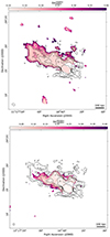 |
Fig. A.1. Spectral index error map between 54 and 144 MHz (top) and between 144 and 380 MHz (bottom). The 54 MHz contours are overlaid in black. |
All Tables
Integrated flux density and spectral indices of 4C 29.41 at 54, 144 and 380 MHz.
All Figures
|
Fig. 1. Radio maps of A1213 at different frequencies. Left: 54 MHz LOFAR image of A1213 produced with briggs −0.3. The rms noise is ∼3 mJy beam−1, and white contours are [−3, 3, 6, 12, 24...] × rms. The beam is 22″ × 18″. Central: 144 MHz LOFAR image of A1213 produced with briggs −0.3. The rms noise is ∼100 μJy beam−1, and white contours are [−3, 3, 6, 12, 24...] × rms. The beam is 8″ × 5″. Right: 380 MHz uGMRT image of A1213 produced with briggs −0.3. The rms noise is ∼60 μJy beam−1, and white contours are [−3, 3, 6, 12, 24...] × rms. The beam is 7″ × 5″. |
| In the text | |
|
Fig. 2. High-resolution LOFAR images of A1213. Left: 144 MHz LOFAR-VLBI image of A1213. The image was produced with a restoring beam of 1.5″ × 1.5″, and with an adapted colorscale to enhance the filamentary emission from the tail. Artefacts due to dynamic range issues are still visible in the image. The rms noise is ∼50 μJy beam−1. Right: 144 MHz LOFAR-VLBI image of 4C 29.41, the central radio galaxy of A1213. The image was produced at a resolution of 0.36″ × 0.19″. The largest angular scale for this data is ∼70″, which prevents the detection of the extended tail in the north-east. Contours are from 2σ to highlight the presence of faint emission, with the σ ∼ 45 μJy beam−1 as the rms noise. |
| In the text | |
|
Fig. 3. Spectral index maps of A1213. Left: Spectral index map between 54 and 144 MHz (beam 30″ × 25″). Upper limits are represented with downwards arrows. Only emission above 3σ is visible. Overlaid in black are 54 MHz contours. The bottom-left panel is a zoom on the eastern part of the tail. Right: Spectral index map between 144 and 380 MHz (beam 24″ × 19″). Only emission above 3σ is visible. Overlaid in black are 54 MHz contours. In both images, the emission to the north and south of 4C 29.41 is affected by calibration artefacts at 144 and 380 MHz and has been masked. |
| In the text | |
|
Fig. 4. Radio emission from LOFAR at 144 MHz (red) overlaid on the optical image of A1213 from SDSS (g-band). Relevant features that we discuss in this work have been labelled. |
| In the text | |
|
Fig. 5. X-ray map of A1213 with overlaid radio contours. Left: LOFAR 54 MHz contours (green) overlaid on the XMM-Newton map in the energy range 0.7−1.2 keV. R200 is ∼1140 kpc, which lies outside of our field of view. Right: Zoom on 4C 29.41 contours as detected at 144 MHz from the 0.3″ resolution image, overlaid on the same XMM-Newton map shown on the left panel. |
| In the text | |
|
Fig. 6. Zoom-in images on member galaxies of A1213. Left: DR10 DESI Legacy Survey optical image of the inner region of A1213. Overlaid are the 54 MHz contours at ∼12″ resolution (red) and the 144 MHz contours at ∼0.3″ resolution (black). Yellow circles denote members of A1213 that could be related to the elongated tail, with their corresponding redshift from SDSS. Right: 144 MHz image at ∼6″ resolution zoomed onto the elliptical galaxy on the north-west region of A1213. The optical galaxy is surrounded by a white square. |
| In the text | |
|
Fig. 7. Spectral curvature (SC) map between 54−144 MHz and 144−380 MHz at ∼20″ resolution. A negative value implies a convex spectral shape. |
| In the text | |
|
Fig. 8. Results of the JP fit on A1213. Left: Regions from which the spectral index was sampled and fit with a JP model, overlaid on the 144 MHz map. Right: Flux density at different frequencies for each region (top) and the corresponding spectral index and the fit with a JP model (bottom). |
| In the text | |
|
Fig. 9. Synchrotron spectrum of 4C 29.41 between 54 and 380 MHz. The orange curve shows the case where no uv-cut was applied while imaging, thus including the contribution of extended emission, that increases the flux density especially at lower frequency. The blue curve shows instead the case with a minimum uv-cut of 1.6 kλ, which roughly corresponds to 2′ (i.e. the larger scale emission is not present). |
| In the text | |
|
Fig. 10. Results of the point-to-point analysis on the central region of A1213. Left: Source-subtracted map of A1213 at 54 MHz, where all sources with LLS < 250 kpc have been removed. It is not possible to remove the whole emission from 4C 29.41, which blends together with the tail and with the roundish emission in the western region. The red grid shows the region of interest of the point-to-point analysis, while the green contours encircle the region where 4C 29.41 is located. Right: Result of the point-to-point analysis between the X-ray and the LOFAR LBA source-subtracted image of A1213. The surface brightness is estimated as the sum of every pixel in each square of the grid, divided by its area. The blue line shows the best fit in the form Y = kX + A, where k = 0.25 ± 0.04 and A = −2.36 ± 0.26. |
| In the text | |
|
Fig. A.1. Spectral index error map between 54 and 144 MHz (top) and between 144 and 380 MHz (bottom). The 54 MHz contours are overlaid in black. |
| In the text | |
Current usage metrics show cumulative count of Article Views (full-text article views including HTML views, PDF and ePub downloads, according to the available data) and Abstracts Views on Vision4Press platform.
Data correspond to usage on the plateform after 2015. The current usage metrics is available 48-96 hours after online publication and is updated daily on week days.
Initial download of the metrics may take a while.