| Issue |
A&A
Volume 693, January 2025
|
|
|---|---|---|
| Article Number | A305 | |
| Number of page(s) | 16 | |
| Section | Galactic structure, stellar clusters and populations | |
| DOI | https://doi.org/10.1051/0004-6361/202451853 | |
| Published online | 28 January 2025 | |
Open cluster dissolution rate and the initial cluster mass function in the solar neighbourhood
Modelling the age and mass distributions of clusters observed by Gaia
1
CENTRA, Faculdade de Ciências, Universidade de Lisboa,
Ed. C8, Campo Grande,
1749-016
Lisboa,
Portugal
2
Laboratório de Instrumentação e Física Experimental de Partículas (LIP),
Av. Prof. Gama Pinto 2,
1649-003
Lisboa,
Portugal
★ Corresponding authors; This email address is being protected from spambots. You need JavaScript enabled to view it.
; This email address is being protected from spambots. You need JavaScript enabled to view it.
; This email address is being protected from spambots. You need JavaScript enabled to view it.
Received:
9
August
2024
Accepted:
10
December
2024
Abstract
Context. The dissolution rate of open clusters (OCs) and the integration of their stars into the Milky Way’s field population have been explored using their age distribution. With the advent of the Gaia mission, there is an exceptional opportunity to revisit and enhance studies covering these aspects of OCs with ages and masses from high-quality data.
Aims. Our aim is to build a comprehensive Gaia-based OC mass catalogue that, combined with the age distribution, allows for deeper investigation of the disruption experienced by OCs within the solar neighbourhood.
Methods. We determined masses by comparing luminosity distributions to theoretical luminosity functions. The limiting and core radii of the clusters were obtained by fitting the King function to their observed density profiles. We examined the disruption process by performing simulations of the build-up and mass evolution of a population of OCs that we compared to the observed mass and age distributions.
Results. Our analysis yielded an OC mass distribution with a peak at log(M) = 2.7 dex (∼500 M⊙) as well as radii for 1724 OCs. Our simulations showed that when using a power-law initial cluster mass function (ICMF), no parameters are able to reproduce the observed mass distribution. Moreover, we find that a skew log-normal ICMF provides a good match to the observations and that the disruption time of a 104 M⊙ OC is t4tot = 2.9 ± 0.4 Gyr.
Conclusions. Our results indicate that the OC disruption time t4tot is about two times longer than previous estimates based solely on OC age distributions. We find that the shape of the ICMF for bound OCs differs from that of embedded clusters, which could imply a low typical star formation efficiency of ≤20% in OCs. Our results also suggest a lower limit of ~60 M⊙ for bound OCs in the solar neighbourhood.
Key words: Galaxy: kinematics and dynamics / open clusters and associations: general / solar neighborhood
© The Authors 2025
 Open Access article, published by EDP Sciences, under the terms of the Creative Commons Attribution License (https://creativecommons.org/licenses/by/4.0), which permits unrestricted use, distribution, and reproduction in any medium, provided the original work is properly cited.
This article is published in open access under the Subscribe to Open model. This email address is being protected from spambots. You need JavaScript enabled to view it. to support open access publication.
1 Introduction
Open clusters (OCs) are gravitationally bound stellar systems typically comprising tens to hundreds of stars that formed together (Lada & Lada 2003). As time progresses, the stars gradually disperse into the general field star population. The dispersion of OCs is influenced by a combination of internal factors, including the cluster’s mass and dynamics, as well as external factors, such as galactic tidal forces, interactions with giant molecular clouds (GMCs), and the influence of spiral arms (Lamers & Gieles 2006).
Mass plays a crucial role in determining the internal dynamics of star clusters and their interactions with external galactic gravitational forces. Because a large fraction of stars (possibly most stars) form in clusters (e.g. Lada & Lada 2003), the process of dissolution is instrumental in shaping both the mass and age distribution of the star cluster population that can be observed, as well as the characteristics of the field star population. Consequently, accurately determining the mass and age distribution of the Milky Way’s star clusters is essential for refining models of their evolution and enhancing understanding of the dissolution processes they undergo.
Prior to the Gaia mission (Gaia Collaboration 2016b) of the European Space Agency (ESA), OC masses had only been published for about 35% of the known clusters in the Milky Way. The majority of the data was provided by Piskunov et al. (2008a) using photometry and astrometry compiled in the ASCC~2.5 catalogue (Kharchenko 2001), which is limited to stars brighter than approximately V ~ 12 mag. This calls for revisiting OC masses using the exquisite data delivered by Gaia, whose various data releases (Gaia Collaboration 2016a, 2018, 2021) have provided astrometric and photometric data for nearly two billion stars, reaching G ~ 20.5 mag and with photometric and astrometric uncertainties at the millimagnitude and sub-milliarcsecond levels, respectively. The data has brought much improved lists of OC members as well as an avalanche of discoveries of new OCs and candidates (e.g. Castro-Ginard et al. 2018; Liu & Pang 2019; Cantat-Gaudin et al. 2019; Sim et al. 2019; Castro-Ginard et al. 2020; Ferreira et al. 2021; Hunt & Reffert 2021) and large-scale determinations of OC distances, ages, extinctions, and other parameters (e.g. Cantat-Gaudin et al. 2018; Bossini et al. 2019; Cantat-Gaudin et al. 2020; Monteiro et al. 2020; Dias et al. 2021; Hunt & Reffert 2023).
However, large-scale Gaia-based determinations of OC masses have been missing until very recently. Almeida, Monteiro, & Dias (2023) (hereafter AMD23) have published a catalogue of masses for 773 OCs. Hunt & Reffert (2024) published a catalogue of OC masses for 3530 clusters where they estimated the age and mass distributions in the Milky Way. On a smaller scale, Cordoni et al. (2023) have determined masses for 78 OCs in their study on the role of binaries in OC evolution. The work presented in this article has different aims and follows a different approach for calculating masses, as we discuss in Sect. 3.3.
In this work, we aim to determine the time scale of the disruption experienced by clusters in the solar neighbourhood. What differentiates this study from previous works (e.g. Lamers et al. 2005a; Anders et al. 2021) is the incorporation of both the age and mass distributions in our analysis as well as the use of Gaia data. Estimates for the disruption parameters have been found previously using the age distribution and N-body simulations of clusters in the tidal field of the Galaxy. Considering that the cluster disruption time depends on the initial mass M of the cluster as tdis = t0(M/M⊙)γ, Boutloukos & Lamers (2003) found γ = 0.6 for clusters within 1 kpc of the Sun, while Baumgardt & Makino (2003) obtained γ = 0.62 from N -body simulations of clusters in the tidal field of the Galaxy at different galacto- centric distances. Lamers et al. (2005a) compared the predicted age distribution to the observed age distribution of OCs in the solar neighbourhood, from the Kharchenko et al. (2005) catalogue, and obtained  Myr and γ = 0.62. However, the previous studies focused solely on the age distribution of clusters due to the lack of a large-scale mass catalogue, so in this work, we aim to expand our understanding by using both the age and mass distributions.
To achieve this, we built a catalogue of OC luminous masses in the Milky Way using data from the Dias et al. (2021) catalogue and Gaia DR2 data. Determining the mass bound to clusters also requires determining their limiting radii. We then generated simulated distributions of age and mass, which we compared to the observations of clusters located within a 2 kpc radius around the Sun, with ages under 1 Gyr. By comparing the simulated and observed distributions for various parameter values, we find the disruption parameters that best match the observations.
This paper is organised as follows. Chapter 2 describes the observational data used in this work. Chapters 3 and 4 present the methods and results for the masses and radii of 1724 OCs and are followed by an investigation of the OC disruption time scale in the solar neighbourhood (Chapters 5 and 6). Chapter 7 closes this work with the conclusions and final considerations.
2 Data
We used the Dias et al. (2021) OC catalogue, which has entries for 1743 objects and is based on Gaia DR2 (Gaia Collaboration 2018). The listed cluster parameters, namely distance, reddening, age, and metallicity were homogeneously derived by applying the cross-entropy isochrone fitting method described in Monteiro et al. (2017) and Monteiro et al. (2021). Additionally, Dias et al. (2021) have provided tables of individual stellar membership probabilities. The lists of members were compiled from other published studies. Some of those studies (Liu & Pang 2019; Castro-Ginard et al. 2020, 2022) do not provide membership probabilities. In these cases, the probabilities were computed by Dias et al. (2021). The membership tables are limited to stars brighter than G ~ 18 mag.
We note that, in principle, we could have adopted the catalogue of Cantat-Gaudin et al. (2020), as both catalogues have comparable sizes and parameters and compile similar lists of members from the same sources. However, as discussed above, membership probabilities are not provided by some sources. In such cases, Cantat-Gaudin et al. (2020) assigned a value of one. Since our analysis uses individual membership probabilities, we opted to use Dias et al. (2021).
We also acknowledge the recent catalogues of OCs published by Hunt & Reffert (2023, 2024), which include many new entries with computed ages, distances, and radii. As these catalogues were published during the final stages of our work, they were not included in our baseline compilation of OCs. Nevertheless, comparisons with these catalogues are provided in Sect. 4.1.2.
Number of OCs per classification.
3 Methods
One of the main aims of this study is the determination of OC masses (i.e. the total mass of stars bound to a cluster). However, cluster masses can be determined from different observables. Using mass-luminosity relations, one may derive cluster masses from stellar luminosity measurements. These mass determinations are often referred to as ‘photometric’ or ‘luminous masses’ and are the ones we determine in this work. Masses derived from kinematic measurements are referred to as ‘dynamical masses’ and ‘virial masses’ (for clusters assumed to be in virial equilibrium). Additionally, one may also consider ‘tidal masses’, which are masses deduced from a cluster’s limiting radius, which is imposed by the balance between the cluster self-gravity and the galactic tidal forces exerted upon the cluster (e.g. Piskunov et al. 2008b).
3.1 Member selection
To produce cluster member lists that are as complete as possible while simultaneously minimising contamination by field stars, as a general rule, we selected stars with membership probabilities above 50%. However, when analysing their colour-magnitude diagrams (CMDs), some clusters still showed clear contamination. In those cases, we increased the membership cut-off to reduce the contamination as much as possible while conserving the clear cluster members. Some clusters had poorly defined CMDs (even when relaxing membership cut-offs). We thus visually inspected the CMDs of all 1743 OCs, with PARSEC isochrones (Bressan et al. 2012) fits over-plotted, and we attributed a classification of P1 (good), P2 (medium), or P3 (worst) based on the dispersion of the cluster sequence and on the quality of the isochrone match. As shown in Table 1, the majority of our sample has a classification of P1. Additionally, as we wanted to compare the masses derived using different Gaia bands, only stars detected in the three bands (G, GBP, and GRP) were considered.
Stars outside the cluster tidal radius are dispersing into the field population and can be found distributed as diffuse tails and coronae around clusters (e.g. Bergond et al. 2001; Dalessandro et al. 2015; Meingast et al. 2021; Guilherme-Garcia et al. 2023; Della Croce et al. 2024). They have kinematic and photometric distributions close to those bound to the cluster. Therefore, separating the bound and unbound populations requires additional criteria. In this work, we make the approximation that all stars within the cluster radius contribute to the bound mass. As can be seen in Sect. 4.1.2, within the uncertainties, this assumption should not significantly affect our results. Therefore, the next step towards building the catalogue of OC masses was to determine their radii.
3.2 Radii determination
For the radii determinations, we fit the King empirical profile (King 1962) to the OC radial density profiles (RDPs). To account for the contamination of foreground and background stars, we followed Küpper et al. (2010) and introduced an additional parameter: c. The modified King function provides the number of stars per pc2 in the form of
 (1)
(1)
where Rk is the limiting radius beyond which the density of stars is indistinguishable from the density of the background; Rc is the core radius, which is the radius for which the density fall to half of the central density; N0 is a scaling factor that reflects the central density of the cluster; and c is the background density, taken as constant.
For simplicity, we assumed that the limiting radius derived from the King profile is equivalent to the tidal radius at which the gravitational attraction of the cluster balances the external tidal forces. However, it is important to acknowledge that this approximation holds true only when the stars within the cluster entirely fill the cluster’s Jacobi radius. This condition may not always be fulfilled, and thus, we discuss the effect of the radius on the derived mass in Sect. 4.2.1. To make the difference clear, we represent the limiting radius as Rk (King radius) instead of as Rt (tidal radius), which is how it is usually found in the literature.
The ring width for the RDPs was chosen as 0.5 pc for clusters where the farthest star was less than 12 pc from the centre, and 1 pc for the other cases. The intention was to avoid under- or oversampling the density profile in clusters with fewer stars.
The profile fits were done with the LMFIT Non-Linear LeastSquares Fitting Python package (Newville et al. 2014). We used the maximum likelihood estimation (MLE) from the emcee method within LMFIT to obtain the King parameters. The uncertainties of each King parameter were taken to be ±σ, as provided by the output of LMFIT. These uncertainties were sampled from the posterior distribution marginalised over the other King model parameters. The convergence of the chains was evaluated based on the value of the integrated autocorrelation time (τ), which is related to the Monte Carlo error (or sampling error), as recommended by Goodman & Weare (2010). In cases where the program raised a warning due to the value of τ, the number of steps was gradually increased (starting from 100 000) until the criterion of τ > 50 was satisfied.
To ensure the results were physically meaningful, the King radius was forced to be larger than the core radius and was allowed to vary between 0.5 and 100 pc. The core radius varied between 0.2 pc and the distance of the farthest star to the centre of the cluster.
3.3 Mass determination
The luminous mass of each OC was determined by comparing the observed luminosity distribution to the theoretical luminosity function (LF) for each cluster. The LFs were obtained from the web interface for the PARSEC1 models of stellar evolution (Bressan et al. 2012; Marigo et al. 2013, 2008; Chen et al. 2015) and were calculated for the Gaia filter passbands of Maíz Apellániz & Weiler (2018) while considering the Kroupa (2001) initial mass function corrected for unresolved binaries of stars and solar metallicity Z = 0.0152.
Our mass determination method consisted of fitting (scaling) the model LF to the observed LF. We started by selecting the model LF with the same age as the cluster being fit and added to it the cluster’s distance modulus and interstellar absorption. We then scaled the model LF to the observed LF. The scaling factor is the number by which the model LF is multiplied that minimises, in a least squares sense, the deviation to the observed LF.
It must be noted that the PARSEC luminosity functions are provided normalised, corresponding to a conceptual population born with 1 M⊙. However, at any given age, the LF no longer corresponds to 1 solar mass since some stars will have died or lost mass. This means that the scale factor obtained above gives the cluster mass at birth. Because we are interested in the mass at the present age of a cluster, a scaling correction had to be applied. To obtain this correction, a population of stars with known masses was generated using the PARSEC web interface, and the mass of the population was evaluated (by summing the masses of each star) at different ages, t, from log(t) = 6.6 to 10, with steps of 0.1 dex. We find that for the age range considered, the mass decreases linearly with log(t), yielding a correction of ϕM = –0.135 log(t) + 1.781, where ϕM is the multiplicative correction to transform the birth mass into the present mass.
As a sanity check, a second mass estimation method was used. In this case, we considered the relation between the area under the observed and theoretical LFs. Dividing the areas under both distributions gave the scaling factor between them, and when multiplied by the scaling correction (ϕM), it yields the mass of the cluster. This method does not capture the mass- (luminosity) and age-dependent fine features of the LF, and it is thus a less accurate approach.
As the PARSEC web interface only allows one bin width to be selected in each retrieval, our freedom of choice for the bin width was limited. Choosing a different bin width for each of the 1743 clusters is impractical, so we chose a common bin width of 0.5 mag for most clusters. However, when the highest count bin had fewer than ten stars, a bin width of 1 mag was used instead. We visually inspected the LF of the 556 clusters in this situation to verify if they were grossly over- or under-sampled.
As previously mentioned, our stellar samples are limited to the apparent magnitude G ≤ 18 mag, which is well within the Gaia completeness limit. However, when the apparent magnitudes are converted to absolute magnitudes and discretised in bins, the last absolute magnitude bins might not be complete. To account for this effect, we removed the last bin of the LFs.
4 Results: Radii, masses, and sample selection
4.1 King radii
During the analysis, we encountered some cases where the fitting of the King profile did not converge. A deeper examination revealed that the density in the peripheral zones of these cluster fields was not zero but was nevertheless very low, of the order of 10–2 stars/pc2. We set this value as the background density, c, and considered that the King radius should not extend into this region. This cut-off reduced the incidence of non-converging radius fits.
Despite this improvement, there were still 15 clusters for which the fits failed, even after trials with other membership and background density cut-offs. We found that their density profiles were either nearly flat or exhibited irregular contours, rendering them unsuitable for King profile fitting. Consequently, these objects were omitted from our sample.
Additionally, a visual inspection of the stellar distributions on the sky showed that four objects (Berkeley 58, Berkeley 59, Blanco 1, and NGC 7789) had incorrectly listed centres that were clearly off the star distributions. These clusters were also removed from the sample. This left us with a sample of 1724 OCs.
Figure 1 presents the distribution of King radii of our OC sample. The full dataset, illustrated in light blue, exhibits a wide bump around 50 pc. Such large radii prompted a more detailed examination. To this end, we excluded clusters with a poorer fit quality (classified as R4; see Sect. 4.1.1) and reevaluated the distribution of radii excluding these clusters, depicted in dark blue. The elimination of these clusters led to the disappearance of the bump. This highlights the importance of careful quality control, which in our case resulted in assigning objects to different quality classes, which we discuss in Sect. 4.1.1.
The cleaned distribution of radii, excluding objects with poor-quality fits, peaks at 5–6 pc and has a median value of 10 pc, consistent with previous literature values (e.g. Piskunov et al. 2007; Kharchenko et al. 2013). The distribution of parameters N0 and c as well as the distribution of core radii, with a median value of 2 pc, are shown in Appendices A and B, respectively.
The uncertainties associated with the King and core radii were determined as detailed in Sect. 3.2. Our analysis revealed that the median fractional uncertainties for the King radius are 47% for the lower bound and 95% for the upper bound. These figures underscore the challenges involved in accurately measuring King radii (defined by the low density regime), especially for clusters with sparse populations. For the core radius (high density regime), as expected the median uncertainties were found to be lower, at 23% for the lower bound and 25% for the upper bound.
To assess the robustness of our fitting procedure, we performed a sanity check by iterating over the King radius in increments of 0.5 pc while allowing the remaining parameters to be optimised by LMFIT for each radius value. For each iteration, we computed the RMS difference between the modelled King profile and the observed stellar density distribution. The parameter set yielding the lowest RMS was selected as the optimal solution. We then compared these results against those obtained through our main method. This comparison revealed that for determinations classified as high quality, the median discrepancy in radii between the two methods was only 2%. However, for the intermediate- and low-quality cases, the differences increased to 15 and 37%, respectively. Further analysis confirmed that a significant portion of the clusters contributing to the bump in the distribution of King radii around 50 pc encountered convergence issues during this process, consistently returning in the maximum King radius value preset in this sanity-check loop.
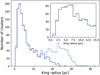 |
Fig. 1 Distribution of King radii for 1724 OCs (in light blue). The dark blue histogram represents the distribution of King radii excluding clusters with poor quality fits (classified as R4; see Sect. 4.1.1). Bin widths were set using Knuth’s rule (Knuth 2006). |
Number of OCs per classification according to the quality of the radii determination.
4.1.1 Radii classification
Our procedure yielded radii for a total of 1724 OCs. However, as previously mentioned, not every determination was deemed reliable, particularly in instances where the observed radial density profiles could not be accurately modelled by a King function.
To address this, we performed a visual classification, assigning each cluster to one of four categories based on the quality of the King profile fit and the congruence of Rk (King radius) and Rc (core radius) with the observed stellar distribution on the tangent plane. These four categories are R1 (best quality), R2 (intermediate quality), R3 (worst quality), and R4 (non-reliable). Specifically, the R3 category includes clusters where the King and core radii are similar, hinting at potential issues with fit convergence. The R4 category primarily includes clusters with excessively large King radii (around 50 pc) or those where the fit is visually unsatisfactory as well as cases where the density distribution does not have a profile suitable for King function fitting. The distribution of clusters across these classifications is given in Table 2. Additionally, Fig. 2 shows a typical example of a cluster classified as R1 (best quality).
4.1.2 Comparison with other studies
We compared the cluster-limiting radii obtained in this study with those given in Tarricq et al. (2022), Just et al. (2023), and Hunt & Reffert (2024), for which we have 109, 938, and 1264 OCs in common, respectively. Tarricq et al. (2022) extended member lists to the outskirts of the clusters, including tails and coronae, resulting in significantly higher numbers of stars with respect to this study. The cluster distances employed also differ from those of Tarricq et al. (2022), who used the values from Cantat-Gaudin et al. (2020), whereas we used values from Dias et al. (2021). Though our study and Tarricq et al. (2022) both fit King density profiles, Tarricq et al. (2022) employed the Markov chain Monte Carlo sampler emcee (Foreman-Mackey et al. 2013) with different criteria and excluded poorly constrained results based on the uncertainties in the radii. In our study, we filtered the results based on the visual quality of the King profile fit.
The radii reported in Hunt & Reffert (2024) are estimates of the OC Jacobi radii. These were determined by summing the individual stellar masses up to the radius at which the stars can remain bound to the cluster based on the collective mass of the enclosed stars and the Galactic tidal forces at the cluster’s position. For clusters that do not fill their Roche volume, these radii are expected to be larger than those derived from the radial density distribution in our study.
The cluster radii used in Just et al. (2023) are a compilation from a series of papers (Kharchenko et al. 2013; Schmeja et al. 2014; Scholz et al. 2015) based on the Milky Way Star Clusters survey (MWSC; Kharchenko 2001), which has a limiting magnitude of V ∼ 14 mag. The radii determinations were performed using the cumulative King profile instead of the linear form in order to mitigate the effects of poor statistics.
The radii distributions obtained by Tarricq et al. (2022); Hunt & Reffert (2024); Just et al. (2023), and this study are presented in Fig. 3. This figure displays histograms as well as Kernel density estimations (KDE) using the gaussian_kde function of the Python Scipy (Virtanen et al. 2020) package with a bandwidth of 2 pc. In general, we note similar distributions of radii, except for those from Tarricq et al. (2022), which tend to be much higher than the other studies, likely reflecting the effect of using stars in cluster coronae and tails in their radii determinations.
A more enlightening picture emerges in Fig. 4, where we present comparisons between the individual radii from each of the catalogues. Here, one can see that even for catalogues with similar radii distributions, the individual values are almost noncorrelated. When comparing only with the ‘silver sample’ from this study (our baseline sample, defined in Sect. 4.3), we found a smaller scatter (mostly from eliminating our higher radii) and that our radii tend to be smaller than the other studies. This might be taken as an indication that the large radii reported in other studies could also be filtered out by employing similar quality cuts. We note that errors will lead mostly to larger radii because they are produced by the low signal (low density) regions. Higher density regions produce clearer cluster signals that are in general not confused with the background field level. In any case, it is clear that the agreement in the distributions does not reflect agreement of the individual values of radii between different catalogues. The large observed scatter highlights the difficulties in determining cluster-limiting radii despite the careful analyses done in these studies and shows that further investigation is needed.
As we show in Sect. 4.2.1, this is not critical for our study since luminous mass determinations turn out not to be much affected by radii errors. However, limiting radii errors will have a critical effect on tidal mass determinations.
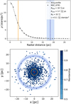 |
Fig. 2 Example of classification R1. (Top) Radial density distribution of OC NGC 6791 (black points) with a fitted King profile (grey solid line). Blue and orange vertical dashed lines represent the King and core radius, respectively. The upper and lower uncertainty of each radius are displayed as the shaded area around each vertical line. The grey horizontal dashed line represents parameter c, which is the background density. (Bottom) Spatial distribution of the cluster stars onto the tangent plane colour-coded by membership probability. Blue and orange circles are at the King and core radius, respectively. |
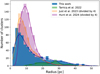 |
Fig. 3 Radii distributions from this work (blue), Tarricq et al. (2022) (green), Hunt & Reffert (2024) (purple), and Just et al. (2023) (orange). KDEs are shown as solid lines. The distributions from Hunt & Reffert (2024) and Just et al. (2023) were divided by four to enable comparison, as the number of OCs is much higher than in the other catalogues. |
 |
Fig. 4 Comparison of the distribution of radii from this work, Tarricq et al. (2022), Hunt & Reffert (2024), and Just et al. (2023). |
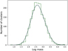 |
Fig. 5 Distribution of the luminous mass, in logarithmic scale. The dark grey solid line is a Gaussian KDE with a bandwidth of 0.18 dex. |
4.2 Luminous mass
We adopted a conservative approach by using the membership cut-offs determined through visual inspection of the colourmagnitude diagrams as described in Sect. 3, which are always above 50%. The resulting distribution of mass, from the G band luminosity functions, is shown in Fig. 5. The logarithmic mass distribution is represented with a histogram and a KDE with a bandwidth of 0.18 dex. The KDE shows a peak at log(M) = 2.7 dex, with a standard deviation of 0.4 dex, which corresponds to a median mass of ~500 M⊙.
4.2.1 Error analysis
In order to investigate the impact of the uncertainties from the King radius on the mass estimates, we computed the mass of each cluster by taking into account the lower and upper bounds of Rk. The mass distributions are displayed in Fig. 6. When considering the lower bound of Rk, the mass is decreased by approximately 8% (median value), whereas it increases by about 6% for the upper bound compared to the mass within Rk.
As an example, we present the cumulative mass distribution for the OC NGC 6791 (Fig. 7) with Rk and its lower and upper bounds. As can be seen, the range of values for the King radius are in the outer regions where less mass is concentrated, and the variation of mass is around 1% in the lower and upper bounds. This illustrates the weak influence of the King radius uncertainties on the luminous mass of the cluster.
To estimate the fitting uncertainties of our mass determination method, we performed a bootstrap using 100 random samples of the magnitude distribution. We adopted the standard deviation as the error of our method for each cluster. Fig. 8 displays the results for the fractional mass error, in the G band, which was obtained using stars within Rk and its lower and upper bounds. The majority of the clusters have a mass error below 4%, with a standard deviation of 3%. The mass errors within the lower and upper bound of Rk are 3 and 5%, respectively.
These results suggest that the uncertainty in the King radius does not significantly impact our mass determinations. It is important to note that these are only the statistical uncertainties associated with our method and not the true uncertainty of each cluster’s mass. Systematic uncertainties related to age, distance, and reddening determinations are not accounted for.
Regarding systematic differences arising from the choice of the IMF, we compared the masses obtained above with those derived using the Chabrier (2003) log-normal IMF. Within the magnitude limit and distance range of our sample, the mass differences range from approximately 10% for closer clusters to 4% for clusters beyond ~1 kpc. This distance-dependent difference arises because lower-mass stars (the regime where the differences between the Chabrier and Kroupa IMFs are most pronounced) are more detectable at closer distances. The differences in OC masses obtained using the two IMFs provide an estimate of the systematic uncertainties involved. Further details on this comparison are provided in Appendix C.
Additionally, if we account for the escape of a fraction of low-mass stars due to mass-segregated evaporation, the systematic error could increase to approximately 20%, assuming about half the stars below ~0.4 M⊙ have escaped. The exact value would depend on the cluster’s dynamical state.
Finally, we also note that another source of uncertainty in our mass determinations arises from the contribution of binary stars. Binary fractions and mass ratios vary within the tidal radius, depending on the cluster’s dynamical state (e.g. Albrow 2024), potentially further influencing the mass estimates. We proceeded with these caveats in mind and provide further discussion on their impact on the OC dissolution time scale in Sect. 7.
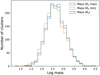 |
Fig. 6 Distribution of the luminous masses determined using only stars inside Rk (grey) and its lower and upper bound (orange and blue, respectively). |
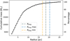 |
Fig. 7 Cumulative mass distribution for OC NGC 6791. The vertical dashed-dotted lines represent Rk (grey), its lower bound (orange), and upper bound (blue). |
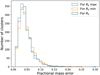 |
Fig. 8 Distribution of the fractional mass error for masses determined using only stars inside Rk (grey) and its lower and upper bound (orange and blue, respectively). |
4.2.2 Consistency assessment
To further assess the consistency of our mass determination method, we determined the mass using the GBP and GRP Gaia bands. Relative to masses determined from the G band, there is a normalised median difference of 3 and 5% for the GBP (Fig. 9, in blue) and GRP bands (Fig. 9, in orange), with associated standard deviations of 18 and 20%, respectively. Essentially, the mass determinations using different bands yields similar results.
In addition, we compared our primary mass determination method with the sanity-check method described in Sect. 3.3 for the same band. The mean mass difference between the two methods (Fig. 9, green) is 6%, with a standard deviation of 13%. Notably, our main method consistently yields lower mass estimates for the clusters. This method is more sensitive to the LF morphology, particularly for cases where cluster parameters such as age or distance are imprecisely determined or when there is incomplete data. In contrast, the validation method is less susceptible to these factors, as previously mentioned.
The observed mass discrepancies between methodologies and bands align closely with the typical mass error of 6%, affirming the robustness of our mass determination approach. Given that the results obtained from the GBP and GRP bands were only used as a validation check, the G band-derived masses are regarded as the main estimations.
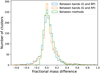 |
Fig. 9 Fractional mass difference for the mass determined using the G and GBP bands (blue), G and GRP bands (orange), and the adopted method and a sanity check (in green). |
Number of clusters per classification according to the quality of the mass determination.
4.2.3 Mass classification
As a further validation step and in order to evaluate the reliability of mass determinations and exclude low-quality results, we classified the 1724 OCs based on the quality of the agreement between the observed and modelled luminosity distributions. A preliminary sorting of clusters was performed using the RMS of the fit and followed by visual classification into three categories: M1 (best), M2, and M3 (worst), as shown in Table 3.
The clusters assigned to the M3 category have mass determinations deemed to be unreliable and significant disparities between the observed magnitude distribution and the theoretical LF. Additionally, a supplementary category, denoted as MX, was established for clusters featuring poorly populated or undefined colour-magnitude diagrams. This classification includes all OCs previously categorised as P3. Clusters assigned to the MX category have poor quality CMDs, rendering their mass determinations invalid. An illustrative example of an M1 classification is presented in Fig. 10.
4.2.4 Comparison with other studies
Figure 11 presents a comparison of our results with the available large catalogues of OC masses from Just et al. (2023), AMD23, and Hunt & Reffert (2024). In the last two catalogues, masses were derived by integrating the mass function constructed using individual stellar masses. The first catalogue provides tidal masses estimated from the galactic tidal forces exerted on the cluster-limiting radii, as detailed in Piskunov et al. (2008b).
There is a general agreement between our masses and the photometric masses from AMD23 and Hunt & Reffert (2024) despite being determined using a different method. However, we observed a tendency for higher masses in Hunt & Reffert (2024), especially in the massive end. This tendency has been noted by Hunt & Reffert (2024) in their comparison with the masses from AMD23 and which they ascribed to their additional corrections for Gaia incompleteness. Given that Gaia DR2 is essentially complete for the G < 18 mag cut adopted here and by AMD23, it is possible that Hunt & Reffert (2024) have slightly over corrected their OC masses, which employ fainter stars.
However, when comparing our masses with those from Just et al. (2023), individual masses display notable discrepancies for most clusters. We note that their (tidal) masses are proportional to  , which makes them highly affected by uncertainties in the tidal radius, Specifically, their error distribution exhibits a mean value of 93% with a standard deviation of 48% (see Fig. 5 of Just et al. 2023). For these reasons, and at least until better radius determinations become available, we consider the luminous masses to be more reliable.
Figure 12 shows the distribution of masses of the four catalogues. Again, a general agreement with AMD23 and Hunt & Reffert (2024) can be observed, with the mass distributions peaking at ~2.6–2.7. We also note that, with respect to this study, the mass distribution of AMD23 is tighter, and that of Hunt & Reffert (2024) is broader. The tidal masses of Just et al. (2023) follow a much broader distribution with the peak at lower masses.
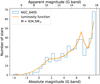 |
Fig. 10 Magnitude distribution of NGC 6405 (for stars with membership >0.7) with the luminosity function (orange line) scaled to match the observed density distribution (blue histogram). The error is displayed as the shaded orange area. The bin width is 0.5 pc. |
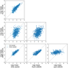 |
Fig. 11 Comparison of individual masses from AMD23, Just et al. (2023), and Hunt & Reffert (2024) with the masses determined in this work. |
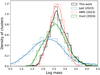 |
Fig. 12 Mass distributions from this work, AMD23, Just et al. (2023), and Hunt & Reffert (2024). The KDEs are represented as solid lines. |
4.3 Sample selection
Given the quality classifications described above, we established two sub-samples. The first, labelled the ‘gold sample’, contains only clusters classified as best quality across all three categories (P1, R1, M1). The second sample, denoted as the ‘silver sample’, includes clusters with intermediate to high quality classifications (i.e. classifications 1 and 2 for photometry, radius, and mass). The gold sample contains 153 OCs (9%), while the silver sample contains 713 OCs (41%). It should be emphasised that the gold sample is entirely contained within the silver sample.
The age and distance distributions of each sample are presented in Fig. 13. These distributions show that the silver sample is distributed in a manner similar to the full sample, indicating the absence of apparent biases resulting from the quality-based selections used to generate the silver sample. In contrast, the gold sample is manifestly small, displaying a much more limited spatial coverage. For these reasons, we adopted the silver sample as our baseline for investigating the OC mass distribution and disruption time scale in the solar neighbourhood.
The age distribution in Fig. 13 shows a marked decline in the number of OCs older than approximately 1 Gyr. While this decrease is expected due to cluster disruption, we cannot rule out that part of it is due to the incompleteness of older, fainter clusters (Moitinho 2010; Moreira et al. 2024). Therefore, we limited our analysis to OCs up to 1 Gyr.
Another prominent feature in the age distribution is the peak at young ages, around log(age) ∼7.1. This peak is also seen in the catalogue of Cantat-Gaudin et al. (2020), but it is not observed in the catalogues of Hunt & Reffert (2023) and Cavallo et al. (2024). The reality of this peak is unclear, with Anders et al. (2021) attributing it to an increased cluster formation rate 6– 20 Myr ago, while Cavallo et al. (2024) attribute it to an artefact caused by red and faint contaminants in isochrone fits. Additionally, ∼20 Myr corresponds to the end of violent relaxation and the rapid dispersal associated with the gas expulsion phase of young clusters (Shukirgaliyev et al. 2019), which could lead to the observed decrease in the number of clusters just after 20 Myr. To avoid this source of uncertainty, we only considered clusters older than 20 Myr when analysing cluster dispersion.
We analysed the spatial completeness of the silver sample following the approach in Moreira et al. (2024). For this, we divided the sample into concentric rings with steps of 450 pc and in three age groups: log(age) ≤ 8.0, 8.0 < log(age) ≤ 8.6 and 8.6 < log(age) ≤ 9.0. The age limits were chosen to have a balanced number of clusters in each group. The radial density profiles for each group are displayed in the bottom panel of Fig. 14. The distributions on the Galactic plane are presented in Fig. 15.
In a complete sample, we would expect the density to remain roughly constant in our immediate neighbourhood. However, as shown in the top panel of Fig. 14, the density decreases with increasing distance. The trend is also observed for the full sample, as thoroughly discussed in Moreira et al. (2024), and it persists in our silver sample.
At young ages, OCs are well-known tracers of spiral arms (e.g. Dias & Lépine 2005; Cantat-Gaudin et al. 2020), and thus they present a structured distribution, as seen in Fig. 15. At intermediate and higher ages, the structure fades, and the distribution appears more homogeneous. The clumpy structures and irregular density profiles for younger clusters make it hard to assess completeness. Nevertheless, given the large variations seen in the density profiles (Fig. 14), observing consistent decreases in density profiles across all age subsets suggests uniform selection effects across different ages. From the spatial distributions (Fig. 15), we observed that beyond a 2 kpc limit, the distributions include regions that are no longer sampled, with larger radii featuring empty areas. For this reason, we restricted our analyses to within 2 kpc.
It is important to emphasise that since the density profiles of the different age groups exhibit a similar decrease with the (cylindrical) distance to the Sun, their ratios remain largely unaffected by incompleteness. We note that we are not referring to the absolute numbers of clusters but to the rate at which they decrease with distance. Although the samples are incomplete, the fraction of clusters removed by incompleteness appears to be independent of age. This is a relevant point because the effects we study, such as the disruption rate, are expressed as ratios of cluster numbers across different age groups. Consequently, this particular source of incompleteness should not influence the determination of the dissolution rate. Nonetheless, the distance cut-off is necessary to mitigate sampling errors in the low-count regime.
Next, we inspect the mass distribution of the silver sample at different distances presented in Fig. 16. A barrier at 60 M⊙ separating the bulk of the clusters from three to four low-mass and sparsely distributed very close clusters can readily be seen. This suggests a ~60 M⊙ lower-mass limit below which stars cannot remain bound in an OC in the solar neighbourhood. The three to four low-mass objects have few stars and exhibit a super virial velocity dispersion; thus they are likely poor OCs in the final phases of dissolution and are only seen due to their closeness. These objects are, from nearest to farthest, Alessi_13, UPK_606, UPK_385, and UPK_624. A similar mass barrier is also seen in the data of AMD23, who do not include the three low- mass outliers. We note that a selection effect would likely result in a smoother distribution, approximately triangular, extending towards smaller masses across the barrier. However, at this stage, we view the ~60 M⊙ minimum mass more as a well-motivated indication than a definitive claim. A robust determination will require further investigation.
In summary, the curated sample that is used below in our model is the silver sample (all quality flags = 1 or 2) restricted to clusters within 2 kpc of the Sun, with ages between 20 Myr and 1 Gyr, and masses greater than 60 M⊙ . Table 42 lists the studied OCs, their determined radii, masses, uncertainties, and quality flags.
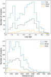 |
Fig. 13 Distribution of age (top) and distance (bottom) for the full sample (blue), silver sample (grey), and gold sample (orange). |
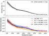 |
Fig. 14 Radial density of the OCs in the silver sample with an age under 1 Gyr (top panel) and for each age sub-sample, normalised to one at the maximum (bottom panel). Poisson errors are represented as shaded areas. |
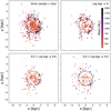 |
Fig. 15 Spatial distribution of the silver sample (top left) and the three age sub-samples projected on the Galactic plane. The black circle is at 2 kpc. The OCs are colour-coded by mass. The X axis points to the galactic centre, and Y points in the direction of the rotation of the Galaxy. The Sun is located at (0,0). |
Determined radii, masses, uncertainties, and quality flags for ten randomly selected OCs.
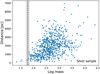 |
Fig. 16 Distribution of distances as a function of the logarithm of mass for the 713 OCs in the silver sample. The grey shaded area represents the interval of masses from 50 to 70 M⊙, with the black dotted line at 60 M⊙ . |
5 Model for the population of dissolving open clusters
Previous studies have shown that the disruption time, tdis , of an OC of mass, Mi, can be described by tdis = t0(Mi/M⊙)γ with a time scale t0 (Boutloukos & Lamers 2003). This time scale depends on the tidal forces of the host galaxy, so it varies between galaxies and is dependent on the position of the cluster in the galaxy. The disruption time (tdis) increases with the cluster initial mass (Lamers et al. 2005a), and this dependence is quantified by the parameter γ, which depends on the concentration of the stellar distribution in the cluster (Lamers et al. 2010).
The strength of the tidal forces increases with proximity to the Galactic centre, making the intensity of disruption dependent on the location of the cluster within the galaxy. However, as the clusters in our sample are located within a few kiloparsecs around the Sun, we assumed the same tidal influence for all clusters. The parameter γ is also assumed to be the same for all clusters, as we did not consider the differences in stellar concentration in the clusters. While estimates for parameters γ and t0 have been made in several studies analysing the OC age distribution, (e.g. Boutloukos & Lamers 2003; Baumgardt & Makino 2003; Lamers et al. 2005a), to the best of our knowledge, the mass distribution has not been considered in previous studies.
To simulate the dissolution rate experienced by OCs in the solar neighbourhood, we followed Lamers et al. (2005a) by employing a simple model that simulates the build-up and mass evolution of a population of OCs across time. The model assumes a constant cluster formation rate and draws their initial masses from an initial cluster mass function (ICMF). As in Lamers et al. (2005a), we adopted a power-law ICMF (Lada & Lada 2003): dN/dM ∝ M−α with α ~ 2, Mmin = 100 M⊙, and Mmax = 3 × 10⁴ M⊙. Later in Sect. 6, we discuss the implications of this choice and explore the adoption of other ICMF functionals.
For the dissolution process, Lamers & Gieles (2006) provided four separate equations for the OC mass loss due to stellar evolution, disruption by the galactic tidal field, spiral arm shocking, and molecular cloud encounters. However, our work is focused on the total disruption of the OCs, and we do not distinguish between different disruption mechanisms. For this reason, we combined the equations from Lamers & Gieles (2006) in a single equation that reproduces the overall mass dependent disruption time.
The expression for the total mass loss is
 (2)
(2)
where Mi is the cluster initial mass in the simulation. This equation reproduces the same mass loss over time as the four separate equations from Lamers & Gieles (2006), with  Gyr and γ = 0.67. As described in Lamers et al. (2005a),
  , so the disruption time scale can also be defined as
  , which results in Eq. (2).
6 Comparison with observations
We ran simulations in a coarse 10 × 9 grid with  ranging from 1 to 10 Gyr in steps of 1 Gyr and γ ranging from 0.1 to 0.9 in steps of 0.1. To quantify the agreement between the simulations and the observational sample (Sect. 4.3), we calculated the likelihood between the predictions and observations, normalising the number of simulated clusters to match the number of observed OCs. We considered the total likelihood as the sum of the loglikelihood from the age and mass distributions, separately. For the standard deviation, we considered Poisson errors
  , where N is the number of OCs in each bin.
6.1 Results with the power-law initial cluster mass function
The optimal range of values for the parameters  and γ considering the age distribution were obtained for a region where
  Gyr with γ between 0.2 and 0.7 and
  Gyr with γ between 0.5 and 0.8. We note that the
  value we find is larger than the 1.3–1.7 Gyr reported in the literature (Lamers et al. 2005a; Lamers & Gieles 2006; Anders et al. 2021). In the top panel of Fig. 17, we present the observed and simulated age distributions for different values of γ given a fixed
  of 2 Gyr where we observe a good agreement.
In contrast, it is not possible to isolate an optimal region in the grid for the masses. In fact, although the region defined above provides good results for the age distribution, the simulated mass distribution does not match the observations for any of the combinations considered. This effect is illustrated in the bottom panel of Fig. 17, where the observed mass distribution is shown with the KDEs of the simulated distributions for different values of γ given a fixed  of 2 Gyr. It is clear that independent of the value of γ, the simulations do not reproduce the observed mass distribution despite the generally good agreement with the ages. For a fixed γ, the effect of changing
  in the mass distribution is small, so none of the combinations in the grid reproduces the observed masses.
This incompatibility was unexpected and was not suggested in previous works (e.g. Lamers & Gieles 2006; Lamers et al. 2005b). Instead, it has been revealed by our new mass catalogue and clearly indicates the need for adjustments in the physical ingredients of the model. We also checked the results using the silver sample within 1.5 kpc and the gold sample within 2 kpc, and we arrived at the same conclusion.
The two key factors influencing the overall shape of the age and mass distributions are the cluster formation rate and the ICMF. Several studies (e.g. Snaith et al. 2015) have indicated that the solar neighbourhood experienced a relatively uneventful star formation history over the past gigayear. Given this, along with the good agreement observed in the age distribution, we find that the discrepancy likely lies in the ICMF.
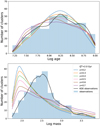 |
Fig. 17 Comparison of the distribution of age (top) and mass (bottom) between the simulations (colour-coded KDEs) and the observations (blue histogram). For the simulations, we considered the power-law ICMF, |

6.2 Exploring alternative forms for the initial cluster mass function
The power-law ICMF of Lada & Lada (2003) has been widely adopted to simulate the initial mass distribution of OC populations in the Milky Way. In particular, it was adopted in Lamers & Gieles (2006); Lamers et al. (2005b) for studying the disruption time scales of OCs. However, this ICMF was determined for embedded clusters, a large fraction of which will not survive the gas expulsion phase (e.g. Lada & Lada 2003; Baumgardt & Kroupa 2007; Shukirgaliyev et al. 2017). In this view, it cannot be taken for granted that the surviving OCs will have the same mass distribution when they emerge from their parent molecular clouds.
Indeed, Parmentier et al. (2008) addressed the difference between the embedded and non-embedded cluster mass functions. They defined the ICMF as the mass function of star clusters right after the effects of gas expulsion have ended (<20 Myr Shukirgaliyev et al. 2017, 2019). In their model, they found that the ICMF can differ from the embedded counterpart, with the shape depending on the star formation efficiency. For a (massindependent) star formation efficiency of 20%, the embedded power-law mass function becomes a bell-shaped ICMF. At efficiencies of ~40%, the shape of the embedded mass function is preserved.
In their study of the minimum mass of bound clusters in different galaxies, Trujillo-Gomez et al. (2019) describe the (non-embedded) ICMF as a power-law ICMF with an exponential truncation at both the high- and low-mass ends that effectively creates a bell-like shape:

with β = −2. For the solar neighbourhood, they find that Mmin = 1.1 × 10² M⊙ and Mmax = 2.8 × 10⁴ M⊙ which are the minimum and maximum mass scales, respectively.
The effect of adopting the ICMF proposed by Trujillo- Gomez et al. (2019) in our model is presented in Fig. 18. While we found good fits to the age distribution, we observed that this ICMF also does not reproduce the observed mass distribution. We note, however, that Trujillo-Gomez et al. (2019) set their ICMF parameters β, Mmin, and Mmax using pre-Gaia masses from Lamers et al. (2005a) based on the Kharchenko et al. (2005) OC catalogue (plus unpublished masses provided by H. Lamers, private communication).
We thus proceeded to estimate the Mmin and Mmax parameters of the ICMF using our sample of masses. Since our sample includes few very young clusters, we used clusters younger than 50 Myr to have enough data (108 OCs in the silver sample) to make a meaningful analysis. Because clusters at this age have already lost some mass, we cannot directly determine the ICMF from the observed distribution. To take this into account, we performed a grid search of the optimal Mmin and Mmax in several runs of the model until 50 Myr. We used  Gyr and γ = 0.6, which provided good fits for the age distribution. The best fits correspond to Mmin ~ 500 M⊙ and Mmax ~ 1000 M⊙, where a variation of about 20% for these parameters still results in a mass distribution that is compatible with the observations. The fit is presented in Fig. 19, where the original ICMF from Trujillo-Gomez et al. (2019) is also presented for comparison. With the optimal parameters, the functional has a shape that more resembles an asymmetric log-normal with a turnover at the typical clusters mass ~500 M⊙. In this sense, the turnover parameter (Mmin) does not define a minimum cluster mass but a typical mass instead.
The truncated power-law ICMF with Mmin ~ 500 M⊙ and Mmax ~ 1000 M⊙ provides a much better fit to the mass distribution of young clusters. However, we found that the number of high-mass clusters was underestimated, and the low-mass clusters were overestimated. This is not totally unexpected given the asymmetry apparent in Fig. 19.
To take this asymmetry into account, we tested a skew lognormal distribution, which has three parameters: skewness α, location (which is the mean when α = 0), and scale (standard deviation when α = 0. See Azzalini & Capitanio 2002). We used the SciPy stats.skewnorm function to draw cluster masses. We found that the best fit was obtained with α = 2, location = 2.3, and scale = 0.5. As seen in Fig. 19, the best fit is broadly similar to the truncated power law, also with a mode ∼500 M⊙ , but it produces a higher number of high-mass clusters. We refer to this skewed log-normal ICMF as the ‘adopted ICMF’, and we use it in the next section.
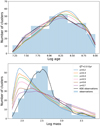 |
Fig. 18 Comparison of the distribution of age (top) and mass (bottom) between the simulations (colour-coded KDEs) and the observations (blue histogram with fitted black KDE) considering |

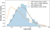 |
Fig. 19 Distribution of the logarithm of mass for OCs with an age under 50 Myr and simulated distribution of masses using different ICMFs: Trujillo-Gomez et al. (2019), Trujillo-Gomez et al. (2019) with Mmin ~ 500 M⊙ and Mmax ~ 1000 M⊙, and the adopted ICMF (skewed lognormal with α = 2, location = 2.3, and scale = 0.5). |
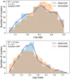 |
Fig. 20 Comparison of the distribution of age (top) and mass (bottom) between the simulations (orange) and the observations (blue) considering |

6.3 Results with the adopted initial cluster mass function
We ran the same grid as before for a first estimate of the optimal values for  and γ using the adopted ICMF. We found good agreement with the observations for (
 ,γ) = (3, 0.7); (3, 0.8); and (4, 0.8). We then ran a thinner grid with 0.1 Gyr steps in
  and 0.05 steps in γ and found the optimal value at
  Gyr and γ = 0.7. The uncertainty was taken as the standard deviation of ten bootstrap samples. The results are presented in Fig. 20. One can see that the model successfully reproduces the general characteristics of the age and mass distributions, such as the location of the peaks and broadness. However, the observed number of intermediate mass clusters (∼500-600 M⊙) is higher. At this stage, we could not determine the cause of this difference, that is, whether it is due to the selection function of the data or a missing ingredient in the model. Although we feel inclined towards the first possibility, this is a matter we are currently investigating, and our findings will be presented in a follow-up work. A check using OCs within a shorter distance (under 1.5 kpc) showed similar trends, with the best values for
  found close to 3 Gyr and γ around 0.6–0.7.
In any case, two results emerged from this analysis. The first is a strong indication that the initial mass distributions for embedded clusters and OCs are substantially different. Qualitatively, the ICMF is bell shaped, which suggests a massindependent star formation efficiency of the order of 20% or lower (Parmentier et al. 2008). The second result is  Gyr, and it is about twice the value of previous estimates, which were based on a power-law ICMF and used only the age distribution of OCs (Lamers et al. 2005a; Anders et al. 2021). This brings the disruption time scale closer to the larger disruption times found in N-body simulations (Baumgardt & Makino 2003; Portegies Zwart et al. 1998). This suggests that the disruption due to interactions with GMCs and spiral arms, while still the dominant channel of cluster disruption, may not be as strong as previously thought (Lamers & Gieles 2006).
7 Conclusions
In this study, we have built a Gaia-based catalogue of luminous masses for a sample of 1724 OCs in the solar neighbourhood by comparing their luminosity distributions to theoretical luminosity functions. Our luminous mass distribution peaks at log(M) = 2.7 dex.
Determining the masses required the preceding step of determining the cluster radii. The King (‘limiting’) and core radii were determined by fitting the King density profile to the observed profile of each cluster. Comparison between the Tarricq et al. (2022), Hunt & Reffert (2024), and Just et al. (2023) catalogues illustrates how hard the determination of cluster King limiting radii is, with large differences of the individual radii between catalogues. Nevertheless, our analysis shows that the uncertainties for the King radii do not have a significant impact on our luminous mass determinations.
Our analysis revealed a general agreement with the photometric masses from AMD23 and Hunt & Reffert (2024), with a trend for higher masses in Hunt & Reffert (2024), which could be due to over-correction for Gaia incompleteness. In contrast, significant discrepancies were observed when we compared our luminous masses with the (tidal) masses from Just et al. (2023), which are highly affected by uncertainties in the tidal radius. Given these findings, we deem the luminous masses more reliable.
To study the mass loss rate in OCs, we simulated the build-up and mass evolution of a population of clusters following Lamers & Gieles (2006). The model has three main ingredients: a cluster formation rate, which was assumed to be constant; an ICMF; and disruption parameters ( , and γ). Using the widely employed power-law ICMF, we obtained good fits to the age distribution, as was found in previous studies (e.g. Lamers & Gieles 2006; Anders et al. 2021), although with longer dissolution times. However, the simulated mass distribution does not agree with the observations in any combination of the parameters. As our model starts from the moment clusters emerge from the parent molecular clouds, we conjecture that the power-law distribution that had been determined for embedded clusters might not be a good description of the initial masses of bound OCs.
Following previous indications that the ICMF may be bell shaped (Parmentier et al. 2008; Trujillo-Gomez et al. 2019), we find that a skew log-normal ICMF provides a good match to the observations. The difference with respect to a power-law distribution of the embedded counterparts could indicate a typical star formation efficiency of ≤20% in solar neighbourhood clusters (Parmentier et al. 2008). Finally, we find indications of a lower limit of ∼60 M⊙ for bound stellar clusters in the solar neighbourhood.
We note two caveats of this study: (1) systematic uncertainties in the mass determinations could lead to overestimations of OC masses by up to 20%, primarily due to the escape of low-mass stars through mass-segregated evaporation. The exact impact depends on the cluster’s dynamical state. Correcting for this effect would likely reduce the value of t4 . However, additional simulations indicate that this reduction would not lower t4 below ∼2.4 Gyr. (2) Variations in binary star fractions and mass ratios within the tidal radius could further affect the mass estimates.
Some questions also remain open. Most noticeably, an excess of intermediate mass OCs are not explained by the model. This may be due to data selection effects. In an era of continuous reports of new OC discoveries, the assessment of the OC selection function and its dependence on distance, age, and mass is badly needed. For this, stringent quality control of the growing sample of OCs and their memberships is essential. Finally, we note that more robust determinations of OC-limiting radii will be crucial for determining dynamical-based masses for comparison. Addressing these caveats and open questions will be the focus of our following studies.
Data availability
Table 4 is available at the CDS via anonymous ftp to cdsarc.cds.unistra.fr (130.79.128.5) or via https://cdsarc.cds.unistra.fr/viz-bin/cat/J/A+A/693/A305.
Acknowledgements
We thank the anonymous referee for their constructive comments which have contributed to improve this paper. This work was partially supported by the Portuguese Fundação para a Ciência e a Tecnologia (FCT) through the Portuguese Strategic Programmes UIDB/FIS/00099/2020 and UIDP/FIS/00099/2020 for CENTRA. D.A. acknowledges support from the FCT/CENTRA PhD scholarship UI/BD/154465/2022. This research has made use of data from the European Space Agency (ESA) mission Gaia, processed by the Gaia Data Processing and Analysis Consortium (DPAC). We also thank Lorenzo Cavallo for insightful comments and suggestions.
Appendix A Distribution of N0 and c
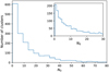 |
Fig. A.1 Distribution of parameter N0. There are 35 OCs with N0 above 80 which were not displayed to allow an easier visualisation. |
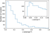 |
Fig. A.2 Distribution of parameter c. There are 53 OCs with c above 1 star/ pc2 which were not displayed to allow an easier visualisation. |
Appendix B Comparison of core radii with Tarricq et al. (2022)
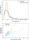 |
Fig. B.1 Distribution of parameter Rc . (Top) Distribution of core radii from this work (blue) and from Tarricq et al. (2022) (orange) with fitted Gaussian KDEs. (Bottom) Individual comparison of the core radii, for the 109 OCs in common with the full sample (dark blue) and 63 in common with the silver sample (light blue). The 1:1 ratio line is plotted as the orange dashed line. |
Appendix C Comparison with results using the Chabrier (2003) IMF
In this appendix, we assess the systematic differences in our results that would arise from adopting the Chabrier (2003) IMF instead of the Kroupa (2001) IMF. To this end, we replicated the mass determination procedure described in Sect. 3.3, selecting the Chabrier (2003) IMF in the PARSEC web interface.
Figure C.1 plots the fractional difference in the mass determinations (Kroupa minus Chabrier) as a function of distance. It shows that, except for a few isolated points, the difference systematically decreases from about −10% to 4% for distances under approximately 1 kpc, and remains at around 4% beyond that. This distance dependence arises because at closer distances, low-mass stars are included in the luminosity functions, enhancing the regime where the differences between the Chabrier and Kroupa IMFs are most pronounced. The distribution of the fractional mass differences is presented in Fig. C.2.
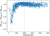 |
Fig. C.1 Fractional mass difference between the photometric masses determined using luminosity functions sampled from the Kroupa (2001) and Chabrier (2003) IMFs, plotted as a function of distance. The dashed line indicates the distance limit of the sample used in our model. |
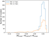 |
Fig. C.2 Distribution of the fractional mass difference for a sample cut at 5 kpc (blue) and at 2 kpc (orange). |
We note that the differences observed here were determined from luminosity function fits that assume no selective mass loss due to dynamical evolution. Therefore, there is a systematic effect due to dynamical evolution that is not being quantified in this analysis.
Since the objective of determining masses was to use them for estimating the disruption time scale, t4 , we reran our model using the masses derived with the Chabrier IMF. We obtained very similar results for the disruption parameters, with the optimal values being  Gyr and γ = 0.68 ± 0.03, compared to
  Gyr and γ = 0.70 ± 0.03 obtained with the Kroupa IMF.
References
- Albrow, M. D. 2024, MNRAS, 528, 6211 [NASA ADS] [CrossRef] [Google Scholar]
- Almeida, A., Monteiro, H., & Dias, W. S. 2023, MNRAS, 525, 2315 [NASA ADS] [CrossRef] [Google Scholar]
- Anders, F., Cantat-Gaudin, T., Quadrino-Lodoso, I., et al. 2021, A&A, 645, L2 [NASA ADS] [CrossRef] [EDP Sciences] [Google Scholar]
- Azzalini, A., & Capitanio, A. 2002, J. R. Stat. Soc. Ser. B Stat. Methodol., 61, 579 [Google Scholar]
- Baumgardt, H., & Kroupa, P. 2007, MNRAS, 380, 1589 [NASA ADS] [CrossRef] [Google Scholar]
- Baumgardt, H., & Makino, J. 2003, MNRAS, 340, 227 [NASA ADS] [CrossRef] [Google Scholar]
- Bergond, G., Leon, S., & Guibert, J. 2001, A&A, 377, 462 [NASA ADS] [CrossRef] [EDP Sciences] [Google Scholar]
- Bossini, D., Vallenari, A., Bragaglia, A., et al. 2019, A&A, 623, A108 [NASA ADS] [CrossRef] [EDP Sciences] [Google Scholar]
- Boutloukos, S. G., & Lamers, H. 2003, MNRAS, 338, 717 [NASA ADS] [CrossRef] [Google Scholar]
- Bressan, A., Marigo, P., Girardi, L., et al. 2012, MNRAS, 427, 127 [NASA ADS] [CrossRef] [Google Scholar]
- Cantat-Gaudin, T., Jordi, C., Vallenari, A., et al. 2018, A&A, 618, A93 [NASA ADS] [CrossRef] [EDP Sciences] [Google Scholar]
- Cantat-Gaudin, T., Krone-Martins, A., Sedaghat, N., et al. 2019, A&A, 624, A126 [NASA ADS] [CrossRef] [EDP Sciences] [Google Scholar]
- Cantat-Gaudin, T., Anders, F., Castro-Ginard, A., et al. 2020, A&A, 640, A1 [NASA ADS] [CrossRef] [EDP Sciences] [Google Scholar]
- Castro-Ginard, A., Jordi, C., Luri, X., et al. 2018, A&A, 618, A59 [NASA ADS] [CrossRef] [EDP Sciences] [Google Scholar]
- Castro-Ginard, A., Jordi, C., Luri, X., et al. 2020, A&A, 635, A45 [NASA ADS] [CrossRef] [EDP Sciences] [Google Scholar]
- Castro-Ginard, A., Jordi, C., Luri, X., et al. 2022, A&A, 661, A118 [NASA ADS] [CrossRef] [EDP Sciences] [Google Scholar]
- Cavallo, L., Spina, L., Carraro, G., et al. 2024, AJ, 167, 12 [NASA ADS] [CrossRef] [Google Scholar]
- Chabrier, G. 2003, PASP, 115, 763 [Google Scholar]
- Chen, Y., Bressan, A., Girardi, L., et al. 2015, MNRAS, 452, 1068 [Google Scholar]
- Cordoni, G., Milone, A. P., Marino, A. F., et al. 2023, A&A, 672, A29 [NASA ADS] [CrossRef] [EDP Sciences] [Google Scholar]
- Dalessandro, E., Miocchi, P., Carraro, G., Jílková, L., & Moitinho, A. 2015, MNRAS, 449, 1811 [Google Scholar]
- Della Croce, A., Dalessandro, E., Livernois, A., & Vesperini, E. 2024, A&A, 683, A10 [NASA ADS] [CrossRef] [EDP Sciences] [Google Scholar]
- Dias, W. S., & Lépine, J. R. D. 2005, ApJ, 629, 825 [NASA ADS] [CrossRef] [Google Scholar]
- Dias, W. S., Monteiro, H., Moitinho, A., et al. 2021, MNRAS, 504, 356 [NASA ADS] [CrossRef] [Google Scholar]
- Ferreira, F. A., Corradi, W. J. B., Maia, F. F. S., Angelo, M. S., & Santos, Jr., J. F. C. 2021, MNRAS, 502, L90 [NASA ADS] [CrossRef] [Google Scholar]
- Foreman-Mackey, D., Hogg, D. W., Lang, D., & Goodman, J. 2013, PASP, 125, 306 [Google Scholar]
- Gaia Collaboration (Brown, A. G. A., et al.) 2016a, A&A, 595, A2 [NASA ADS] [CrossRef] [EDP Sciences] [Google Scholar]
- Gaia Collaboration (Prusti, T., et al.) 2016b, A&A, 595, A1 [NASA ADS] [CrossRef] [EDP Sciences] [Google Scholar]
- Gaia Collaboration (Brown, A. G. A., et al.) 2018, A&A, 616, A1 [NASA ADS] [CrossRef] [EDP Sciences] [Google Scholar]
- Gaia Collaboration (Brown, A. G. A., et al.) 2021, A&A, 649, A1 [NASA ADS] [CrossRef] [EDP Sciences] [Google Scholar]
- Goodman, J., & Weare, J. 2010, Commun. Appl. Math. Comput. Sci., 5, 65 [Google Scholar]
- Guilherme-Garcia, P., Krone-Martins, A., & Moitinho, A. 2023, A&A, 673, A128 [NASA ADS] [CrossRef] [EDP Sciences] [Google Scholar]
- Hunt, E. L., & Reffert, S. 2021, A&A, 646, A104 [NASA ADS] [CrossRef] [EDP Sciences] [Google Scholar]
- Hunt, E. L., & Reffert, S. 2023, A&A, 673, A114 [NASA ADS] [CrossRef] [EDP Sciences] [Google Scholar]
- Hunt, E. L., & Reffert, S. 2024, A&A, 686, A42 [NASA ADS] [CrossRef] [EDP Sciences] [Google Scholar]
- Just, A., Piskunov, A. E., Klos, J. H., Kovaleva, D. A., & Polyachenko, E. V. 2023, A&A, 672, A187 [NASA ADS] [CrossRef] [EDP Sciences] [Google Scholar]
- Kharchenko, N. V. 2001, Kinematika i Fizika Nebesnykh Tel, 17, 409 [NASA ADS] [Google Scholar]
- Kharchenko, N. V., Piskunov, A. E., Röser, S., Schilbach, E., & Scholz, R. D. 2005, A&A, 438, 1163 [NASA ADS] [CrossRef] [EDP Sciences] [Google Scholar]
- Kharchenko, N. V., Piskunov, A. E., Schilbach, E., Röser, S., & Scholz, R.-D. 2013, A&A, 558, A53 [NASA ADS] [CrossRef] [EDP Sciences] [Google Scholar]
- King, I. 1962, AJ, 67, 471 [Google Scholar]
- Knuth, K. H. 2006, arXiv e-prints [arXiv:physics/0605197] [Google Scholar]
- Kroupa, P. 2001, MNRAS, 322, 231 [NASA ADS] [CrossRef] [Google Scholar]
- Küpper, A. H. W., Kroupa, P., Baumgardt, H., & Heggie, D. C. 2010, MNRAS, 407, 2241 [NASA ADS] [CrossRef] [Google Scholar]
- Lada, C. J., & Lada, E. A. 2003, ARA&A, 41, 57 [Google Scholar]
- Lamers, H., & Gieles, M. 2006, A&A, 455, L17 [NASA ADS] [CrossRef] [EDP Sciences] [Google Scholar]
- Lamers, H., Gieles, M., Bastian, N., et al. 2005a, A&A, 441, 117 [NASA ADS] [CrossRef] [EDP Sciences] [Google Scholar]
- Lamers, H., Gieles, M., & Portegies Zwart, S. F. 2005b, A&A, 429, 173 [NASA ADS] [CrossRef] [EDP Sciences] [Google Scholar]
- Lamers, H., Baumgardt, H., & Gieles, M. 2010, MNRAS, 409, 1 [Google Scholar]
- Liu, L., & Pang, X. 2019, ApJS, 245, 32 [NASA ADS] [CrossRef] [Google Scholar]
- Maíz Apellániz, J., & Weiler, M. 2018, A&A, 619, A180 [Google Scholar]
- Marigo, P., Girardi, L., Bressan, A., et al. 2008, A&A, 482, 883 [NASA ADS] [CrossRef] [EDP Sciences] [Google Scholar]
- Marigo, P., Bressan, A., Nanni, A., Girardi, L., & Pumo, M. L. 2013, MNRAS, 434, 488 [Google Scholar]
- Meingast, S., Alves, J., & Rottensteiner, A. 2021, A&A, 645, A84 [NASA ADS] [CrossRef] [EDP Sciences] [Google Scholar]
- Moitinho, A. 2010, IAU Symp., 266, 106 [NASA ADS] [Google Scholar]
- Monteiro, H., Dias, W. S., Hickel, G. R., & Caetano, T. C. 2017, New A, 51, 15 [NASA ADS] [CrossRef] [Google Scholar]
- Monteiro, H., Dias, W. S., Moitinho, A., et al. 2020, MNRAS, 499, 1874 [NASA ADS] [CrossRef] [Google Scholar]
- Monteiro, H., Barros, D. A., Dias, W. S., & Lépine, J. R. D. 2021, Front. Astron. Space Sci., 8, 62 [NASA ADS] [CrossRef] [Google Scholar]
- Moreira, S., Moitinho, A., Silva, A., & Almeida, D. 2024, A&A in press, https://doi.org/10.1051/0004-6361/202450369 [Google Scholar]
- Newville, M., Stensitzki, T., Allen, D. B., & Ingargiola, A. 2014, Astrophysics Source Code Library [record ascl:1606.014] [Google Scholar]
- Parmentier, G., Goodwin, S. P., Kroupa, P., & Baumgardt, H. 2008, ApJ, 678, 347 [NASA ADS] [CrossRef] [Google Scholar]
- Piskunov, A. E., Schilbach, E., Kharchenko, N. V., Röser, S., & Scholz, R.-D. 2007, A&A, 468, 151 [NASA ADS] [CrossRef] [EDP Sciences] [Google Scholar]
- Piskunov, A. E., Kharchenko, N. V., Schilbach, E., et al. 2008a, A&A, 487, 557 [NASA ADS] [CrossRef] [EDP Sciences] [Google Scholar]
- Piskunov, A. E., Schilbach, E., Kharchenko, N. V., Röser, S., & Scholz, R.-D. 2008b, A&A, 477, 165 [NASA ADS] [CrossRef] [EDP Sciences] [Google Scholar]
- Portegies Zwart, S. F., Hut, P., Makino, J., & McMillan, S. L. W. 1998, A&A, 337, 363 [NASA ADS] [Google Scholar]
- Schmeja, S., Kharchenko, N. V., Piskunov, A. E., et al. 2014, A&A, 568, A51 [CrossRef] [EDP Sciences] [Google Scholar]
- Scholz, R. D., Kharchenko, N. V., Piskunov, A. E., Röser, S., & Schilbach, E. 2015, A&A, 581, A39 [NASA ADS] [CrossRef] [EDP Sciences] [Google Scholar]
- Shukirgaliyev, B., Parmentier, G., Berczik, P., & Just, A. 2017, A&A, 605, A119 [NASA ADS] [CrossRef] [EDP Sciences] [Google Scholar]
- Shukirgaliyev, B., Parmentier, G., Berczik, P., & Just, A. 2019, MNRAS, 486, 1045 [NASA ADS] [CrossRef] [Google Scholar]
- Sim, G., Lee, S. H., Ann, H. B., & Kim, S. 2019, J. Korean Astron. Soc., 52, 145 [NASA ADS] [Google Scholar]
- Snaith, O., Haywood, M., Di Matteo, P., et al. 2015, A&A, 578, A87 [NASA ADS] [CrossRef] [EDP Sciences] [Google Scholar]
- Tarricq, Y., Soubiran, C., Casamiquela, L., et al. 2022, A&A, 659, A59 [NASA ADS] [CrossRef] [EDP Sciences] [Google Scholar]
- Trujillo-Gomez, S., Reina-Campos, M., & Kruijssen, J. M. D. 2019, MNRAS, 488, 3972 [NASA ADS] [CrossRef] [Google Scholar]
- Virtanen, P., Gommers, R., Oliphant, T. E., et al. 2020, Nat. Methods, 17, 261 [Google Scholar]
The full table with all 1724 OCs will be available at the CDS.
All Tables
Number of OCs per classification according to the quality of the radii determination.
Number of clusters per classification according to the quality of the mass determination.
Determined radii, masses, uncertainties, and quality flags for ten randomly selected OCs.
All Figures
|
Fig. 1 Distribution of King radii for 1724 OCs (in light blue). The dark blue histogram represents the distribution of King radii excluding clusters with poor quality fits (classified as R4; see Sect. 4.1.1). Bin widths were set using Knuth’s rule (Knuth 2006). |
| In the text | |
|
Fig. 2 Example of classification R1. (Top) Radial density distribution of OC NGC 6791 (black points) with a fitted King profile (grey solid line). Blue and orange vertical dashed lines represent the King and core radius, respectively. The upper and lower uncertainty of each radius are displayed as the shaded area around each vertical line. The grey horizontal dashed line represents parameter c, which is the background density. (Bottom) Spatial distribution of the cluster stars onto the tangent plane colour-coded by membership probability. Blue and orange circles are at the King and core radius, respectively. |
| In the text | |
|
Fig. 3 Radii distributions from this work (blue), Tarricq et al. (2022) (green), Hunt & Reffert (2024) (purple), and Just et al. (2023) (orange). KDEs are shown as solid lines. The distributions from Hunt & Reffert (2024) and Just et al. (2023) were divided by four to enable comparison, as the number of OCs is much higher than in the other catalogues. |
| In the text | |
|
Fig. 4 Comparison of the distribution of radii from this work, Tarricq et al. (2022), Hunt & Reffert (2024), and Just et al. (2023). |
| In the text | |
|
Fig. 5 Distribution of the luminous mass, in logarithmic scale. The dark grey solid line is a Gaussian KDE with a bandwidth of 0.18 dex. |
| In the text | |
|
Fig. 6 Distribution of the luminous masses determined using only stars inside Rk (grey) and its lower and upper bound (orange and blue, respectively). |
| In the text | |
|
Fig. 7 Cumulative mass distribution for OC NGC 6791. The vertical dashed-dotted lines represent Rk (grey), its lower bound (orange), and upper bound (blue). |
| In the text | |
|
Fig. 8 Distribution of the fractional mass error for masses determined using only stars inside Rk (grey) and its lower and upper bound (orange and blue, respectively). |
| In the text | |
|
Fig. 9 Fractional mass difference for the mass determined using the G and GBP bands (blue), G and GRP bands (orange), and the adopted method and a sanity check (in green). |
| In the text | |
|
Fig. 10 Magnitude distribution of NGC 6405 (for stars with membership >0.7) with the luminosity function (orange line) scaled to match the observed density distribution (blue histogram). The error is displayed as the shaded orange area. The bin width is 0.5 pc. |
| In the text | |
|
Fig. 11 Comparison of individual masses from AMD23, Just et al. (2023), and Hunt & Reffert (2024) with the masses determined in this work. |
| In the text | |
|
Fig. 12 Mass distributions from this work, AMD23, Just et al. (2023), and Hunt & Reffert (2024). The KDEs are represented as solid lines. |
| In the text | |
|
Fig. 13 Distribution of age (top) and distance (bottom) for the full sample (blue), silver sample (grey), and gold sample (orange). |
| In the text | |
|
Fig. 14 Radial density of the OCs in the silver sample with an age under 1 Gyr (top panel) and for each age sub-sample, normalised to one at the maximum (bottom panel). Poisson errors are represented as shaded areas. |
| In the text | |
|
Fig. 15 Spatial distribution of the silver sample (top left) and the three age sub-samples projected on the Galactic plane. The black circle is at 2 kpc. The OCs are colour-coded by mass. The X axis points to the galactic centre, and Y points in the direction of the rotation of the Galaxy. The Sun is located at (0,0). |
| In the text | |
|
Fig. 16 Distribution of distances as a function of the logarithm of mass for the 713 OCs in the silver sample. The grey shaded area represents the interval of masses from 50 to 70 M⊙, with the black dotted line at 60 M⊙ . |
| In the text | |
|
Fig. 17 Comparison of the distribution of age (top) and mass (bottom) between the simulations (colour-coded KDEs) and the observations (blue histogram). For the simulations, we considered the power-law ICMF, |
| In the text | |
|
Fig. 18 Comparison of the distribution of age (top) and mass (bottom) between the simulations (colour-coded KDEs) and the observations (blue histogram with fitted black KDE) considering |
| In the text | |
|
Fig. 19 Distribution of the logarithm of mass for OCs with an age under 50 Myr and simulated distribution of masses using different ICMFs: Trujillo-Gomez et al. (2019), Trujillo-Gomez et al. (2019) with Mmin ~ 500 M⊙ and Mmax ~ 1000 M⊙, and the adopted ICMF (skewed lognormal with α = 2, location = 2.3, and scale = 0.5). |
| In the text | |
|
Fig. 20 Comparison of the distribution of age (top) and mass (bottom) between the simulations (orange) and the observations (blue) considering |
| In the text | |
|
Fig. A.1 Distribution of parameter N0. There are 35 OCs with N0 above 80 which were not displayed to allow an easier visualisation. |
| In the text | |
|
Fig. A.2 Distribution of parameter c. There are 53 OCs with c above 1 star/ pc2 which were not displayed to allow an easier visualisation. |
| In the text | |
|
Fig. B.1 Distribution of parameter Rc . (Top) Distribution of core radii from this work (blue) and from Tarricq et al. (2022) (orange) with fitted Gaussian KDEs. (Bottom) Individual comparison of the core radii, for the 109 OCs in common with the full sample (dark blue) and 63 in common with the silver sample (light blue). The 1:1 ratio line is plotted as the orange dashed line. |
| In the text | |
|
Fig. C.1 Fractional mass difference between the photometric masses determined using luminosity functions sampled from the Kroupa (2001) and Chabrier (2003) IMFs, plotted as a function of distance. The dashed line indicates the distance limit of the sample used in our model. |
| In the text | |
|
Fig. C.2 Distribution of the fractional mass difference for a sample cut at 5 kpc (blue) and at 2 kpc (orange). |
| In the text | |
Current usage metrics show cumulative count of Article Views (full-text article views including HTML views, PDF and ePub downloads, according to the available data) and Abstracts Views on Vision4Press platform.
Data correspond to usage on the plateform after 2015. The current usage metrics is available 48-96 hours after online publication and is updated daily on week days.
Initial download of the metrics may take a while.