| Issue |
A&A
Volume 693, January 2025
|
|
|---|---|---|
| Article Number | A246 | |
| Number of page(s) | 12 | |
| Section | Numerical methods and codes | |
| DOI | https://doi.org/10.1051/0004-6361/202451831 | |
| Published online | 22 January 2025 | |
Machine-learning approach for mapping stable orbits around planets
1
Grupo de Dinâmica Orbital e Planetologia, São Paulo State University, UNESP,
Guaratinguetá,
CEP 12516-410,
São Paulo,
Brazil
2
Eberhard Karls Universität Tübingen,
Auf der Morgenstelle, 10,
72076
Tübingen,
Germany
3
LESIA, Observatoire de Paris, Université PSL, CNRS, Sorbonne Université,
5 place Jules Janssen,
92190
Meudon,
France
★ Corresponding author; This email address is being protected from spambots. You need JavaScript enabled to view it.
Received:
7
August
2024
Accepted:
3
December
2024
Abstract
Context. Numerical N-body simulations are typically employed to map stability regions around exoplanets. This provides insights into the potential presence of satellites and ring systems.
Aims. We used machine-learning (ML) techniques to generate predictive maps of stable regions surrounding a hypothetical planet. This approach can also be applied to planet-satellite systems, planetary ring systems, and other similar systems.
Methods. From a set of 105 numerical simulations, each incorporating nine orbital features for the planet and test particle, we created a comprehensive dataset of three-body problem outcomes (star-planet-test particle). Simulations were classified as stable or unstable based on the stability criterion that a particle must remain stable over a time span of 104 orbital periods of the planet. Various ML algorithms were compared and fine-tuned through hyperparameter optimization to identify the most effective predictive model. All tree-based algorithms demonstrated a comparable accuracy performance.
Results. The optimal model employs the extreme gradient boosting algorithm and achieved an accuracy of 98.48%, with 94% recall and precision for stable particles and 99% for unstable particles.
Conclusions. ML algorithms significantly reduce the computational time in three-body simulations. They are approximately 105 times faster than traditional numerical simulations. Based on the saved training models, predictions of entire stability maps are made in less than a second, while an equivalent numerical simulation can take up to a few days. Our ML model results will be accessible through a forthcoming public web interface, which will facilitate a broader scientific application.
Key words: methods: numerical / planets and satellites: dynamical evolution and stability
© The Authors 2025
 Open Access article, published by EDP Sciences, under the terms of the Creative Commons Attribution License (https://creativecommons.org/licenses/by/4.0), which permits unrestricted use, distribution, and reproduction in any medium, provided the original work is properly cited.
This article is published in open access under the Subscribe to Open model. This email address is being protected from spambots. You need JavaScript enabled to view it. to support open access publication.
1 Introduction
The population of known exoplanets has grown every year and has prompted extensive research of the stability of extrasolar planetary systems. To investigate the potential existence of satellites or ring systems around these exoplanets, numerical N -body simulations are frequently employed. These simulations map the stability regions around a planet based on a grid of orbital parameters as initial conditions for the N -body integration.
Several studies expanded this analysis to various contexts in different gravitational settings. Hunter (1967) examined the stability of satellites orbiting Jupiter under the influence of solar gravity. Their findings indicate that the stable zone for prograde motion extends to 0.45 of a Hill radius (rHill), while for retrograde motion, it extends to 0.75 rHill. Neto & Winter (2001) investigated the gravitational capture in the Sun-Uranus-satellite system. They employed a diagram of initial conditions of semimajor axis versus eccentricity to identify stable regions around Uranus, considering particles with various initial inclinations and arguments of pericenter.
Holman & Wiegert (1999) numerically investigated the stability of S-type and P-type planet orbits around a binary star system and treated the planet as a test particle. Their work resulted in an empirical expression for the critical semimajor axis of a stable particle that initially is on a circular and planar orbit, relating it to binary distance, mass ratio, and eccentricity. The authors analyzed a range of binary mass ratios µ = [0–0.9] and eccentricities e = [0–0.8].
Domingos et al. (2006) examined the stability of hypothetical satellites orbiting extrasolar planets with a mass ratio µ = 10−3. They derived an empirical expression for the stability boundary in prograde (i = 0°) and retrograde (i = 180°) orbits, formulated in terms of the Hill radius and the eccentricities of the planet and the satellite.
Rieder & Kenworthy (2016) conducted N -body simulations to analyze the stability of a potential ring system around the candidate planet J1407b, thereby imposing constraints on the orbital and physical parameters of this system. For the PDS110b system, Pinheiro & Sfair (2021) performed millions of numerical simulations of the three-body problem with the aim to refine parameters that remained undefined based on observational data, including the mass and eccentricity of an unseen secondary companion, as well as the ring inclination and radial size.
While these studies provided valuable insights, conducting numerical simulations like this for many systems incurs substantial computational expense. To address this challenge, a novel method to expedite this process involves the use of MachineLearning (ML) algorithms. In this approach, N -body simulations generate a dataset for training ML models, which can then predict outcomes for unseen data more efficiently.
The identification of stability regions using ML methods was demonstrated in previous studies. Tamayo et al. (2016) applied ML algorithms to predict the stability of tightly packed planetary systems that consist of three planets orbiting a central star. Their models achieved a predictive accuracy of 90% over the test set, and they were faster by three orders of magnitude than direct N-body simulations.
Tamayo et al. (2020) developed the code called stability of planetary orbital configurations classifier (SPOCK). This ML model is capable of predicting the stability of compact systems with three or more planets. This approach is 105 times faster than numerical simulations.
Cranmer et al. (2021) introduced a probabilistic ML model that predicts the stability of compact multiplanet systems with three or more planets, including when these systems are likely to become unstable. This model demonstrates an accuracy higher by two orders of magnitude in predicting instability times than analytical estimators.
Expanding on this approach, Lam & Kipping (2018) employed deep neural networks to predict the stability of initially coplanar circular P-type orbits for circumbinary planets. Their method achieved an accuracy of at least 86% for the test set, which further demonstrates the potential of ML in analyzing orbital stability.
Building upon the successes of previous ML applications in orbital stability analysis, we propose using this approach to predict a stable-region map surrounding a single-planet system. This method can also be extended to analyze the stability of other analogous systems, such as planet-satellite pairs, planetary rings, and binary minor planets, provided they lie within the trained parameter space of the ML model.
We conducted a series of dimensionless numerical simulations involving an elliptical three-body problem (star, planet, and a particle orbiting the planet). Each simulation represents a distinct initial condition within our dataset, which is used to train and evaluate ML algorithms. Expanding on the work of Domingos et al. (2006), our study explores a wide range of orbital and physical parameters, including the mass ratio of the system and several orbital elements of the particle and planet.
This comprehensive approach would be computationally demanding if it were solved purely through numerical simulations, especially when the number of grid parameters to be analyzed is increased. Running a single three-body problem may be relatively fast, but a broader set of initial conditions may significantly increase computational costs. This highlights the advantages of our ML method.
This paper is structured as follows: Section 2 introduces key concepts and methods for our analysis and introduces the ML algorithms. Section 3 describes our numerical model and the dataset preparation. Section 4 describes our treatment of imbalanced classes. Section 5 evaluates the performance of our ML algorithms. Section 6 compares the predictions made by our best-performing ML model with the results from Domingos et al. (2006) and Pinheiro & Sfair (2021), and with a stability map of the Saturn satellites. Finally, Section 7 presents our concluding remarks and implications of this study.
2 Supervised learning
This section presents the fundamental concepts and techniques for our study. These definitions and approaches are referenced and compared throughout the subsequent sections, particularly in our results and discussion.
Supervised learning includes the desired solution (labels) in the training data. These labels can be composed of a continuous numerical value (regression task) or of discrete values that represent different classes (classification task).
Classification tasks are techniques that use training samples (or instances) during the learning process to develop a generalization of the classes and predict given unknown new instances. We address binary classifications of stable and unstable particles to predict stability maps within a specific planetary system.
The dataset was split into three subsets: training, validation, and test data. The training data were used by the algorithm to find the best generalization features for different classes. The validation data provided an unbiased evaluation of the model effectiveness, and they were used to tune the model hyperparameters and thresholds, select the best ML algorithm, and detect under- and overfitting (Shalev-Shwartz & Ben-David 2014).
The cross-validation technique involves partitioning the training data into subsets. Specifically, we split the training data into five subsets. Subsequently, we trained and evaluated the model on distinct subsets, which was followed by averaging the outcomes to estimate the unbiased error on the training set of the model (Fushiki 2011).
After training several models with different configurations multiple times on the reduced training set and evaluating them through a cross-validation, we identified the best-performing model. Subsequently, we retrained the selected model using the complete training dataset and evaluated the final performance of the ML model using holdout data (test dataset).
We divided our work into five main steps, as shown in Figure 1, which sketches the workflow of our method. The process began with the generation of a dataset from numerical simulations. We then addressed the issue of imbalanced classes through resampling techniques. Using a cross-validation, we tuned the hyperparameter and explored optimal threshold values to establish the best-configuration model. The final step involved assessing the performance of the best model.
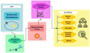 |
Fig. 1 Flowchart illustrating the workflow. |
2.1 Hyperparameter tuning
Hyperparameters are specific algorithm parameters that must be set prior to the training process, and the model performance directly depends on them (Weerts et al. 2020). The search for the best hyperparameters was carried out in two different ways. The first way was a grid search, and the second way was a random search. Both ways were validated using a cross-validation.
The grid search systematically explored all possible combinations of the hyperparameters. In contrast, the random search randomly selected some combinations that were evaluated, which is useful for an extensive number of potential combinations.
2.2 Threshold tuning
In binary classification tasks, classifier algorithms in general employ a default threshold value of 0.5. This means that when the probability that an instance is in a positive class is ≥0.5, it is assigned to the positive class; otherwise, it is classified as negative. However, for an imbalanced dataset, it is generally inappropriate to use 0.5 as the threshold values (Zou et al. 2016).
The receiver operating characteristic (ROC) curve is a frequently employed tool for determining the optimal threshold value (Géron 2022). The ROC curve is a probability curve that plots the true-positive rate (hereafter referred to as recall) versus the false-positive rate for different threshold probabilities from 0 to 1. Figure 2 provides an illustrative example of ROC curves for three hypothetical models with varying performance levels, and also the ROC curve of our best performance ML model (see Sect. 5).
The true-positive rate is the ratio of positive instances that are correctly predicted, while the false-positive rate represents the fraction of negative instances that are incorrectly predicted as positive. The ROC curve always begins at point (0,0), where the threshold is 1, signifying that all instances are predicted as negative. It ends at (1,1), where the threshold is 0, indicating that all instances are predicted as positive.
The area under the curve (AUC) represents the area under the ROC curve. It provides a measure of the model ability to differentiate classes. In a perfect model (exemplified by the black curve in Figure 2), the positive class is always predicted with an accuracy of 100%, regardless of the threshold parameter. This results in an AUC of 1.
Good predictors tend to have an AUC value close to 1. For instance, the green curve in Figure 2 has an AUC of 0.77, indicating that the model has a probability of 77% of successfully distinguishing between positive and negative classes. The dashed red line represents the ROC curve of our best-performing ML model with an AUC of 0.998. This model is discussed in Section 5.
The reference line (dashed gray line) represents an AUC of 0.5, signifying that the model cannot differentiate between classes. This results in random guesses for predictions. Conversely, the blue curve represents a poorly performing model with an AUC of 0.23, where the majority of positive instances are predicted as negative.
The optimal threshold (the black dot in Figure 2) can be determined as the point closest to the upper left corner of the ROC curve (0,1), or the point that maximizes the distance from the reference line where the true-positive rate is high and the false-positive rate is low.
The concepts and methods outlined in this section provide the framework for our subsequent analysis. We refer to these definitions and compare their effectiveness below, in particular when we evaluate our results and discuss their implications.
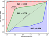 |
Fig. 2 ROC curve representation of three hypothetical models. The black curve behaves like an ideal model, and the green and blue curves represent good and poor classifiers, respectively. The dashed gray line is the reference line. The red curve represents the performance of our best-performing ML model. |
2.3 Classification algorithms
We tested eight distinct ML algorithms to determine the optimal approach: nearest neighbors, naive Bayes, artificial neural network, and the tree-based methods decision tree, random forest, XGBoost, light gradient boosting machine (LightGBM), and histogram gradient boosting. Finally, we ran a genetic algorithm to verify our findings.
Because all tree-based algorithms demonstrated better and comparable performance, we focused our analysis on these methods. With the exception of decision tree, all other tree-based classifiers are ensemble methods that use a group of weaker learners (in this case, an ensemble of decision trees) to enhance their predictions. The collective perspective of a group of predictors yields better predictions than a single predictor (Géron 2022). We give further details of the fundamental concepts of each of these tree-based algorithms in Appendix A.
3 Dataset preparation
In this section, we detail the method with which we investigated the orbital stability of a three-body problem (star, planet, and particle) through an ensemble of dimensionless numerical simulations. Each simulation represents a distinct initial condition for a hypothetical planetary system.
We began by defining the mass parameter µ as
 (1)
(1)
where mp and Ms are the masses of the planet and star, respectively.
The survey including 4150 confirmed exoplanets from Schneider et al. (2011), reveals that 95.71% of them have an equivalent µ ≤ 10−2, and 2.05% of these have µ < 10−5. Thus, we restricted our analysis to this range of mass parameters, and within this, we adopted a random uniform distribution.
Throughout all numerical simulations, the star and planet masses were set by Ms = 1 − µ and mp = µ, respectively. The planet semimajor axis was set to 1, and its collision radius (rc) was defined as 5% of the Hill radius (RHill) computed at the pericenter,
 (2)
(2)
This choice for rc means that 55.6% of the planets in the catalog of Schneider et al. (2011) have a collision radius that is smaller than 5% of their Hill radii, as shown in the histogram in Figure 3.
The planet eccentricity (ep ) and true anomaly ( fp ) were randomly uniformly sampled within the specified ranges of ep = [0−0.99] and fp = [0°–360°]. The remaining orbital elements for the planet inclination (ip ), arguments of pericenter (ϖp), and longitude of the node (Ωp) were set to zero.
The test particle was modeled orbiting a planet and gravitationally disturbed by the star. We adopted a random uniform distribution to select the particle orbital initial conditions for the semimajor axis from 1.1 rc to 1 RHill, an eccentricity from 0 to 0.99, an inclination between 0° and 180°, and arguments of pericenter, longitude of the node, and true anomaly ranging from 0° to 360°.
We numerically integrated using the REBOUND package and the IAS15 integrator (Rein & Spiegel 2015) for a time span of 104 orbital periods of the planet. We recorded every time when the particle collided with the planet or was ejected from the system, which occurred when the particle reached a hyperbolic orbit (eccentricity e ≥ 1) or when its semimajor axis was a > 1.
In total, we ran 105 numerical systems, and the overall outcome was as follows: 11.83% of the particles remained stable throughout the entire integration, while 88.17% were unstable. Of the unstable particles, 53.56% collided with the planet, and 46.44% were ejected from the system.
The outcomes of the numerical simulations were used to build a dataset for training ML algorithms. This dataset consisted of nine features that were the initial conditions of each numerical simulation: the mass ratio of the system, semimajor axis, inclination, argument of pericenter, and longitude of the node of the particle, and the eccentricity and true anomaly of the planet and the particle. We labeled each initial condition with the numerical results as either a stable or an unstable system.
Figure 4 shows four histograms of the number of numerical simulations in relation to the particle semimajor axis (upper left panel), the eccentricity (upper right panel), the inclination (lower left panel), and the planet eccentricity (lower right panel).
As the eccentricity of the planet increases, the number of stable systems is slightly reduced. Nevertheless, we can find stable particles even for highly eccentric planets. The particle eccentricity has a more distinct effect on the number of stable systems: no stable orbits are found for e > 0.8. This is expected since particle orbits experience stronger gravitational disturbances at their pericenters, which increases the quantity of particles that collide.
The number of stable systems is also strongly influenced by the inclination of particles relative to the orbital plane of the planet. Our set contains no stable systems for inclinations between 80° and 110°, and retrograde systems tend to have more stable orbits than prograde ones.
A significant number of collisions occurs closer to the planet, and the number of stable systems increases with the initial particle distance, reaching a peak at 0.3 RHill. After this peak, the quantity of stable systems declines, and only a few systems remain stable beyond 0.7 RHill ; most particles are ejected.
Other features, such as the mass ratio of the system, the argument of pericenter, the longitude of the ascending node, and the true anomaly, were distributed regularly across the range of their parameters.
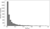 |
Fig. 3 Histogram of the number of confirmed planets in units of their Hill radius from a survey consisting of 4150 different planets (Schneider et al. 2011). |
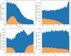 |
Fig. 4 Histogram of the distribution of stable (orange) and unstable (blue) systems across the range of particle semimajor axes (upper left panel), particle eccentricities (upper right panel), particle inclinations (lower left panel), and planet eccentricities (lower right panel). |
4 Imbalanced class
The numerical results demonstrate that the classes are disproportionate in the dataset by a factor 1:10, with the unstable class being much larger than the stable class. This imbalance could lead to biases in the classification and might impair the effectiveness of the various classifier algorithms when they try to generalize (Zheng et al. 2015). ML algorithms typically assume that classes are evenly distributed, which can causes the minority class to be classified poorly (Kumar & Sheshadri 2012; Carruba et al. 2023).
Resampling the training data is one strategy that can be used to solve this problem. One option is undersampling. This technique removes instances from the majority class. The weakness of this method is that it may lose information by removing part of the data (Mohammed et al. 2020). Another resampling process is oversampling, which involves increasing the size of the minority class until the classes are balanced. We tested the performance of four different types of oversampling: random oversampling, the synthetic minority oversampling technique (SMOTE), borderline SMOTE, and adaptive synthetic sampling (ADASYN). In Appendix B, we provide additional details on the key concepts of each of these resampling techniques.
According to Carruba et al. (2023), a severely imbalanced dataset can occur when the class ratio is 1:100, and in this scenario, resampling methods may be necessary. After testing the performance of our algorithms with various resampling techniques, we observed a marginal improvement, except for the LightGBM, which increased by 13% in identifying stable particles. This was achieved solely through the resampling technique, and no hyperparameters or thresholds were tuned. With this improvement, the LightGBM performance is almost as good as the best-performing model without any resampling.
5 Performance evaluation
Evaluation metrics enable the assessment of the classifier performance. The confusion matrix is a statistical table that maps the prediction results by showing the quantity of correctly and incorrectly predicted data (Stehman 1997). While accuracy measures the rate at which a model correctly predicts, this metric may not be reliable for imbalanced datasets. A confusion matrix displays the actual number of instances for each class in its rows and the predicted number of instances for each class in its columns. It is divided into four categories: true positive (TP) and true negative (TN), where the algorithm correctly predicts positive and negative classes; and false positive (FP) and false negative (FN), where the algorithm incorrectly predicts positive and negative classes.
These four categories are used to measure recall, specificity, precision, F1-score, and accuracy. The accuracy is the ratio of instances that are correctly predicted by the algorithm, given by
 (3)
(3)
The specificity or true negative rate is the ratio of correctly predicted instances within the actual negative class,
 (4)
(4)
and the false-positive rate is given by 1 – Specificity.
The recall or the true-positive rate is the ratio of correctly classified positive instances to the total number of actual positive instances,
 (5)
(5)
The precision is the ratio of actual positive instances within the predicted positive class,
 (6)
(6)
The F1-score combines precision and recall by calculating their harmonic mean,
 (7)
(7)
While accuracy measures the rate at which a model correctly predicts, this metric may not be reliable for imbalanced datasets. The F1 scores measure the overall quality of a model, ranging from 0 to 1, where 1 signifies a model that perfectly classifies instances and 0 indicates a model that fails to classify any instance correctly.
5.1 Results and comparison of different algorithms
The ML outcomes were evaluated using a dataset generated from numerical simulations (see Sect. 3). Our binary approach involved classifying systems as either stable or unstable. The final dataset consisted of 100 000 simulations, divided into three subsets: 80% for training and validation data, and 20% for testing data. In the presence of imbalanced classes and to achieve better performance in classifier algorithms, we tested five distinct resampling methods. We used cross-validation techniques to identify the best hyperparameters, resampling method, and the optimal threshold value for each algorithm.
The best performance among the five algorithms was achieved by XGBoost, without using any resampling techniques, with a threshold value of 0.4, and setting some hyperparameters as follows:
booster = gbtree.Booster is a hyperparameter for the type of boosting model used during the training stage. Gbtree means gradient boosted trees.
eta = 0.2. Eta is the learning rate, and mathematically, it scales the contribution of each tree added to the model.
scale_pos_weight = 0.4. Controls the balance of positive and negative class weights.
max_depth = 8. The maximum depth for each tree.
This result was also verified using the genetic algorithm. Genetic algorithms mimic the process of genetic evolution and are capable of selecting the most optimal algorithm and the best hyperparameters for a given dataset (Chen et al. 2004).
Figure 5 shows the performance of the five algorithms using four distinct metrics. The upper left panel displays the accuracy, and the precision for each class is presented in the upper right panel. The lower left panel shows the recall, and the lower right panel shows the F1-scores. Stable classes are represented by orange bars, and unstable classes are shown with blue bars.
All algorithms demonstrated a comparable accuracy performance. XGBoost achieved the highest accuracy at 98.48%, while Decision Tree exhibited the lowest score at 97.43%, showing a marginal difference of 1.05%.
An important consideration here is that the accuracy measures how correctly the model classifies whether the system is stable or unstable across all predicted data. Therefore, this favorable result may be influenced by the proportion of imbalanced classes, with the quantity of unstable instances being approximately 7.5 times larger than stable ones in our dataset. The algorithms achieved a recall and precision of 99% for all classes, except for the precision of Random Forest and the recall of the Decision Tree algorithm, which were 98%.
In terms of stable class performance, LightGBM and Random Forest achieved the highest precision value. They correctly classified 95% of their predictions. They identified 92 and 88% of the actual stable instances (recall), respectively. XGBoost attained the same percentages for precision and recall, leading to the highest F1-score of 94%, while LightGBM and Random Forest achieved 93 and 92%, respectively.
The area under the ROC curve (AUC) provides a measure of the overall model performance, with a value of 1 representing perfect classification (Figure 2). Table 1 compares the AUC values for each algorithm. XGBoost outperformed other models, closely followed by LightGBM and Histogram Gradient Boosting. The Decision Tree algorithm shows a slightly lower performance than the ensemble methods.
Figure 6 shows the confusion matrices for each algorithm and provides the statistical results from the testing dataset of 20 000 instances. Class 0 represents a stable system, and class 1 is unstable. All algorithms demonstrate a satisfactory performance. Even the lowest-performing model (Decision Tree) correctly predicts at least 19 485 instances.
XGBoost, the highest-accuracy algorithm, misclassified only 303 instances, with a nearly balanced distribution of errors between stable and unstable classes (150 and 153 instances, respectively). It also correctly identified the highest number of stable instances (2211). Random Forest and LightGBM achieved the highest precision for the stable class (0.95). They slightly outperformed XGBoost in this metric.
Random Forest showed the best performance in correctly classifying unstable instances (17 536). However, it also had the highest number of false positives, misclassifying 285 stable instances as unstable. This is nearly twice the error rate of XGBoost for this class.
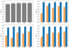 |
Fig. 5 Performance of the best model of the five tested algorithms. The upper panels show accuracy and precision, and the lower panels show recall and F1-score. The stable and unstable classes are represented by orange and blue bars, respectively. The algorithms are abbreviated as follows: DT, RF, HGB, LGBM, and XGB. |
Area under the ROC curve for the best model of each algorithm, sorted in descending order of performance.
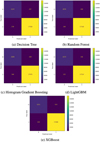 |
Fig. 6 Confusion matrices for the best models of five ML algorithms. |
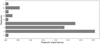 |
Fig. 7 Feature importance derived from the XGBoost model. The orbital elements are denoted as follows: The semimajor axis (a), the eccentricity (e), the inclination (i), the argument of pericenter (ω), the longitude of the node (Ω), and the true anomaly ( f ). Planet-specific parameters are indicated with a subscript p. The mass ratio of the system is represented by µ. |
5.2 Feature importance
An interesting outcome of the XGBoost algorithm is the feature importance, which estimates how effectively each feature contributes to reducing the impurity throughout all the decision tree splits. The feature importance is determined by averaging the importance of each feature across all decision trees, and Figure 7 illustrates the relative importance of features in our classification task.
Particle orbital elements dominate the top three positions. The semimajor axis (a), eccentricity (e), and inclination (i) score 0.3567, 0.2783, and 0.2351, respectively. These findings agree with the distribution patterns observed in Section 3, where we noted significant reductions in stable systems beyond 0.6rHill and the absence of stable particles with inclinations near 90° or eccentricities >0.8. Planet eccentricity ranks fourth in importance (0.0564), followed by the particle argument of pericenter (ω, 0.0274). The remaining features (particle true anomaly ( f ), mass ratio (µ), planet true anomaly ( fp), and particle longitude of node (Ω)) contribute less significantly, with scores ranging from 0.0119 to 0.0110.
These results quantify the relative importance of the orbital parameters in determining the system stability that most significantly influence the dynamical outcomes.
6 Comparative analysis
We applied our best ML model, XGBoost, to predict four distinct diagrams with initial conditions (a × e) with the aim of reproducing the results of Domingos et al. (2006), Pinheiro & Sfair (2021), and those for a particular Saturn moon group known as Inuit. In each diagram, the test particles were uniformly distributed within a range of initial semimajor axes from 1.1 rp to 1 rHill with a step size of ∆a = 0.1 rp, and the initial eccentricities ranged from 0 to 0.5, with ∆e = 0.01.
The XGBoost model, which demonstrated superior performance in our earlier analysis with an accuracy of 98.48%, was tasked with predicting the stability in these specific planetary systems. This approach allowed us to evaluate the generalization capabilities of the model for diverse orbital configurations and to compare its predictions directly with established numerical results.
An entire stability map with ~10000 different initial conditions with numerical simulations requires between two and four days on a single core of an Intel i7-1165G7 processor. The ML predictions, with the saved training, generated a map in 0.5 seconds.
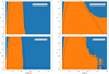 |
Fig. 8 Comparison of numerical simulations (upper panels) and ML predicted outcomes (lower panels) for stable (orange) and unstable (blue) particles. The initial conditions match those from Domingos et al. (2006) for µ = 10−3, with i = 0° (left) and i = 180° (right). The dashed lines represent the analytical expression from Domingos et al. (2006). |
6.1 Comparison with Domingos et al. (2006)
Domingos et al. (2006) numerically simulated multiple stable maps to delineate the boundaries of stable regions surrounding a close exoplanet orbiting its star at a semimajor axis of 0.1 au. They derived an analytical expression for the critical exosatellite semimajor axis as a function of the eccentricity of the satellite and the planet for two different orbital inclinations 0° and 180°.
We reproduced (a × e) diagrams of two different systems explored by Domingos et al. (2006), one on a prograde and the other on a retrograde orbit. The mass ratio of the planet and star was defined as µ = 10−3, with a planet radius rp = 0.05 rHill and orbiting a Sun-like star on a circular orbit.
Figure 8 compares the numerical simulation results with machine-learning predictions. The left panels represent the results for a prograde system, and the right panels show retrograde systems. The performance of our model predictions are summarized in Figure 9, where the dashed lines refers to a prograde system and the solid lines to the retrograde case. The dashed lines represent the analytical expression derived by Domingos et al. (2006).
In the two scenarios, the model accurately classified the main structure of the stable region (orange points), but it showed some discrepancies at the boundaries. For the prograde case, the model closely replicated the stable region, with only minor differences at the edges. The stable region extends to about 0.49 rHill in the numerical and ML results, which agrees well with Domingos et al. (2006). The model achieved an overall accuracy of 95.86%, a precision of 94% for unstable particles and 100% for stable particles, a recall of 100% for unstable particles and 89% for stable particles, and an F1-score of 97% for unstable particles and 94% for stable particles.
The performance comparison of the analytical expression for the critical semimajor axis proposed by Domingos et al. (2006) and our ML model revealed similar results overall. While the equations of Domingos et al. (2006) exhibit a marginally higher accuracy (96.05%) and recall for the stable and unstable classes (91.80 and 98.70%, respectively), our ML model outperforms their results in precision for both classes. Specifically, Domingos et al. (2006) achieved a precision of 97.78% for stable particles and 95.08% for unstable particles, whereas our model achieved a precision of 100% in both classes. The F1-score for the two methods has the same percentage.
For the retrograde case, the model captured the overall larger stable region, extending to about 0.93 rHill. However, it slightly underestimated the stable region extent for eccentricities above 0.3. The ML model also missed some stable particles with semimajor axes beyond 0.8 rHill, in particular, at lower eccentricities.
Despite these limitations, the ML model achieved an accuracy of 86.24%. It outperformed the analytical expression by Domingos et al. (2006), which had an accuracy of 85.04%. Furthermore, the ML model attained a precision of 99% for stable particles and 62% for unstable particles, a recall of 83% for stable particles and 98% for unstable particles. These results yielded F1-scores of 90% for stable particles and 76% for unstable particles. In comparison, the equations of Domingos et al. (2006) achieved slightly lower F1-scores, with 89.26% for stable particles and 74.85% for unstable particles, along with a recall of 80.81% for the stable class and a precision of 59.94% for the unstable class. However, their precision and recall for stable and unstable particles were marginally better, with values of 99.83 and 99.54%, respectively.
These results demonstrate that our model model can accurately predict the general structure of stable regions for prograde and retrograde orbits, but areas for potential improvement are also highlighted, in particular, in capturing fine details at stability boundaries and for highly eccentric orbits in retrograde systems. Even the analytical expression by Domingos et al. (2006), which only applies to µ = 10−3 and inclinations of 0° or 180° failed to classify many stable particles beyond the black line. A further refinement of the model, possibly through an expanded dataset or enhanced feature engineering, could address these minor discrepancies.
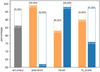 |
Fig. 9 Performance comparison of numerical simulations and machinelearning predictions for prograde (dashed line) and retrograde (solid line) orbits from Domingos et al. (2006). The blue and orange regions represent unstable and stable particles, respectively. |
6.2 Comparison with Pinheiro & Sfair (2021)
Pinheiro & Sfair (2021) studied the stability of a possible ring system around the candidate planet PDS110b. They ran 1.3 × 10⁶ numerical simulations of the three-body problem, each representing a different initial condition. We evaluated the performance of our model for the PDS110b system, specifically considering a scenario in which the planet mass was equivalent to 6.25 Jupiter masses, the eccentricity was 0.2, and the ring inclination was 150°. This scenario corresponds to one of the possible parameters for a retrograde ring system around PDS110b.
Figure 10 shows the numerical and predicted stability maps around PDS110b. Although this system is retrograde, the model performed much better than in the previous example in this case. It achieved an accuracy of 93.68% over ~20 000 predicted initial conditions. The number of stable and unstable instances was almost equivalent, with 5722 actual stable and 14 373 actual unstable instances, respectively.
Figure 11 shows precision, recall, and F1 scores for both classes. The percentages range between 85 and 98%. The slight difference is attributed to the model generalization at the boundary of the stable region, where it misclassified 286 instances as unstable and 984 instances as stable. Some of these misclassifications belong to outlier particles beyond the stable region. Our numerical simulations covered a time span of 104 orbital periods; some of these stable particles might become unstable with longer integration times, however.
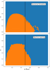 |
Fig. 10 Stability maps for PDS110b. Top panel: numerical simulation results. Bottom panel: ML prediction. The black line represents the minimum radial size for the observed ring as reported by Pinheiro & Sfair (2021). |
6.3 Stability map of the Saturn Inuit satellites
Some irregular Saturn moons are classified into three different groups that are distinguished by their inclination range. We generated a stability map for the Inuit group, where the range of inclination was between 40° and 50°. Table 2 summarizes the orbital elements of the moons belonging to this group.
As another test, we ran ~20 000 numerical simulations of a three-body problem representing the Sun, Saturn (corresponding to µ = 2.857 × 10⁻⁴), and a test particle. The initial orbital inclination of the test particle was set to 45°, and the argument of pericenter, true anomaly, and longitude of node were randomly selected from 0° to 360° using a uniform distribution.
Figure 12 shows the numerical and machine-learning predictions for this example. The black squares represent the satellites belonging to the Inuit group.
This example produced our best performance with an accuracy of 97.57%, along with a precision and recall for the stable class of 97 and 93%, respectively, and with a precision and recall for the unstable class of 98 and 99% (Fig. 13). In total, the ML model incorrectly classified only 470 instances out of ~20 000, and most of them were spread particles at the boundary of the stable region. This good result is reflected in the F1-score, which for both classes reached high values, 95% for the stable class and 98% for the unstable one.
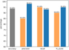 |
Fig. 11 Performance metrics for the PDS110b system prediction. |
Orbital elements of Saturn satellites belonging to the Inuit group.
7 Final remarks
This study demonstrates the efficacy of ML techniques in predicting orbital stability for a hypothetical planet. We used a comprehensive dataset derived from 105 numerical simulations of three-body systems that encompassed a wide range of orbital and physical parameters. These parameters included the mass ratio of the system, the semimajor axis, the inclination, the argument of pericenter, the longitude of the node, the eccentricity, and the true anomaly for the planet and test particles.
Our numerical simulations revealed that 11.83% of the particles remained stable throughout the integration period, while 47.22% collided with the planet and 40.95% were ejected from the system. This imbalanced class distribution necessitated the application of resampling methods to enhance the model performance. We evaluated five ML algorithms: Random Forest, Decision Tree, XGBoost, LightGBM, and Histogram Gradient Boosting, and all algorithms demonstrated a comparable accuracy performance. Through rigorous hyperparameter tuning and threshold optimization, we identified XGBoost as the bestperforming model. It achieved an accuracy of 98.48%. To validate the generalization capabilities of our model, we applied it to reproduce the numerical results of Domingos et al. (2006), Pinheiro & Sfair (2021), and a stability map for the Saturn Inuit group of satellites. The model demonstrated a robust performance and achieved an accuracy of 97.57% for these diverse scenarios. Even though our dataset covered inclinations from 0° to 180°, near i= 180° the stable region exhibited significant sensitivity to minor inclination variations, which resulted in a decreased performance. Additionally, we also tested the performance of our model in the case of Earth (µ = 3×10⁻⁶) and obtained an accuracy of 95.17%.
Our results show the potential of ML algorithms as powerful tools for reducing computational time in three-body simulations in order 105 times faster than traditional numerical simulations. The ability to generate stability maps that cover a wide range of orbital and physical parameters within seconds represents a significant advancement in efficiency compared to traditional numerical methods. The implementation of our model will be made accessible through a public web interface, facilitating its use by the broader scientific community.
As future work, we are refining the model performance, in particular in capturing fine details at the stability boundaries and for highly eccentric orbits and highly retrograde system.
Additionally, we plan to expand the dataset to include more diverse planetary system configurations that might enhance the generalization capabilities of the model and broaden its applicability to a wider range of astrophysical scenarios.
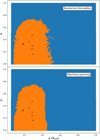 |
Fig. 12 Stability maps for the Saturn Inuit satellites. Top panel: Numerical simulation results. Bottom panel: ML prediction. The black squares represent the actual satellites belonging to the Inuit group. |
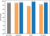 |
Fig. 13 Performance metrics for the Saturn’s Inuit satellites prediction. |
Acknowledgements
We would like to thank the anonymous referee for the constructive comments that greatly improved the manuscript. This research was financed in part by: Coordenação de Aperfeiçoamento de Pessoal de Nível Superior - Brasil (CAPES) - Finance Code 001; Fundação de Amparo a Pesquisa no Estado de São Paulo (FAPESP) - Proc. 2016/24561-0; German Research Foundation (DFG) - Project 446102036.
Appendix A Machine learning algorithms
Here we present the main concepts and characteristics of the tree-based ML algorithms used in this paper.
Decision Tree
Decision Tree, first introduced by Quinlan (1986), classifies instances by splitting them into leaf nodes (Mitchell 1997). This method builds a tree formed by a sequence of several nodes, each with a specific rule (xi < ti), where ti is a threshold value of a single feature (xi) in the ith node (Shalev-Shwartz & Ben-David 2014). The tree starts with the root node, where the data are split into two new subsets and nodes, which can be either a leaf node or a decision node. The leaf or terminal node is where the instance is classified, while the decision node splits the sample again into two new subsets and nodes. This process repeats until the end of the branch.
The choice of feature and best threshold value for each node depends on the impurity of the subsequent two subsets, which can be calculated by estimating the class distribution before and after the split (Géron 2022).
Bagging classifier: Random Forest
Generating a set of classifiers can improve accuracy and robustness. When this approach uses the same training algorithm for every predictor to train different random subsets, the method is called bagging (Géron 2022). The Bagging classifier creates random subsets of the dataset and trains a model on each subset (Breiman 1996). This method returns a combination using a voting scheme of predictions from all predictors.
The bagging algorithm for trees works by iteratively selecting a subset of instances from a training set through bootstrapping, then fitting a tree to these selected instances. Predictions for unseen instances are made by averaging the predictions from all individual trees (Cutler et al. 2011).
Random Forest, introduced by Breiman (2001), is an example of a bagging classifier and an ensemble of Decision Trees. Random Forest reduces the risk of overfitting by decreasing the correlation between trees (Shalev-Shwartz & Ben-David 2014). It trains numerous decision trees using different subsets of the training data. The final prediction is determined by the most voted outputs among these individual decision trees.
Boosting classifiers
Boosting aims to improve the accuracy of any given learning algorithm. This method combines several weak learners into a strong learner and trains predictors sequentially, with each one attempting to rectify the errors of its predecessor (Géron 2022). It uses the residuals of the previous model to fit the next model. The following subsections present an overview of XGBoost, LightGBM, and Histogram Gradient Boosting.
XGBoost
XGBoost (Extreme Gradient Boosting) is a decision tree ensemble developed by Chen & Guestrin (2016) based on the idea of Gradient-Boosted Tree (GBT) by Friedman (2001). It computes the residual of each tree prediction, which are the differences between the actual values and the model predictions. These residuals update the model in subsequent iterations, reducing the overall error and improving predictions (Wade & Glynn 2020).
Unlike sequentially built Gradient-Boosted Trees, XGBoost splits the data into subsets to build parallel trees during each iteration.
XGBoost differs from Random Forest in its training process. It incorporates new trees predicting the residuals of previous trees, and combines these predictions, assigning varying weights to each tree, for the final prediction (Chen & Guestrin 2016).
LightGBM
Light Gradient Boosting Machine (or LightGBM) is a variant of the Gradient-Boosted Tree released in 2016 as part of Microsoft’s Distributed Machine Learning Toolkit (DMTK) project (Ke et al. 2017). The method employs histograms to discretize continuous features by grouping them into distinct bins. LightGBM introduces the leaf-wise growth strategy, which converges quicker and achieves lower residual.
LightGBM provides different characteristics compared to XGBoost, offering alternative benefits that may be more suitable depending on the specific use case. These include improved memory usage, reduced cost of calculating the gain for each split, and reduced communication cost for parallel learning, resulting in lower training time compared to XGBoost. The algorithm also uses the new Gradient-Based One-Sided Sampling (GOSS) and Unique Feature Bundle (EFB) techniques (Ke et al. 2017). GOSS creates the training sets for building the base trees, while EFB groups sparse features into a single feature (Bentéjac et al. 2021).
Histogram Gradient Boosting
Histogram Gradient Boosting is a boosting model inspired by LightGBM. For training sets larger than tens of thousands of instances, this technique, with its histogram-based estimators, proves very efficient and faster than previous boosting methods (Wade & Glynn 2020). Traditional decision trees require long processing times and heavy computation for huge data samples, as the algorithm depends on splitting all continuous values and characteristics (Ibrahim et al. 2023).
Histogram Gradient Boosting streamlines this process by using histograms to bin the continuous instances into a constant number of bins. This approach reduces the number of splitting points to consider in the tree, allowing the algorithm to leverage integer-based data structures (Wade & Glynn 2020). Consequently, this improves and speeds up the tree implementation.
Appendix B Imbalanced class
Random oversampling involves replicating instances randomly within the dataset to achieve a balance in class distribution. This approach may lead to overfitting, and an alternative solution to avoid this is to use the SMOTE.
Chawla et al. (2002) proposed oversampling the minority class by generating "synthetic" instances. Firstly, this method calculates the difference in feature vectors between an instance and its nearest neighbors. In the second step, it multiplies this difference by a random number ranging from 0 to 1, and a new instance is subsequently created by adding this result to the features of the original instance.
Another oversampling technique based on SMOTE is Borderline-SMOTE (Han et al. 2005). This method attempts to identify the borderline of each class and avoids using the outliers (noise points) of the minority class to resample them. The algorithm works with the following steps:
For each instance of the minority class, check which class its nearest neighbors belong to.
Count the number of nearest instances that belong to the majority class.
If all neighbors are from other classes, this point is classified as a noise point, and it is ignored when resampling the data.
If more than half of the neighbors are from other classes, this is a border point. In this case, the algorithm identifies the K nearest neighbors that are of the same class and generates a synthetic instance between them.
If more than half of the neighbors are from the minority class, it is a safe point and the SMOTE technique is applied normally.
The last oversampling approach implemented in this work is ADASYN, which generates synthetic instances for the minority class by considering the weighted distribution of this particular class.
The methodology employed by He et al. (2008) involves an estimation of the impurity of the nearest neighbors ri for each instance in the minority class, given by
 (B.1)
(B.1)
where ∆i is the number of non-minority and K the number of neighbors.
The subsequent step normalizes the ri value as
 (B.2)
(B.2)
where m is the size of the minority class data. This normalized value is then multiplied by the total number of synthetic instances to be generated. This procedure proportions the number of synthetic instances to be created for each minority instance.
References
- Bentéjac, C., Csörgő, A., & Martínez-Muñoz, G. 2021, Artif. Intell. Rev., 54, 1937 [Google Scholar]
- Breiman, L. 1996, Mach. Learn., 24, 123 [Google Scholar]
- Breiman, L. 2001, Mach. Learn., 45, 5 [Google Scholar]
- Carruba, V., Aljbaae, S., Caritá, G., et al. 2023, Front. Astron. Space Sci., 10, 1196223 [NASA ADS] [CrossRef] [Google Scholar]
- Chawla, N. V., Bowyer, K. W., Hall, L. O., & Kegelmeyer, W. P. 2002, J. Artif. Intell. Res., 16, 321 [CrossRef] [Google Scholar]
- Chen, T., & Guestrin, C. 2016, in Proc. 22nd ACM SIGKDD International Conference on Knowledge Discovery and Data Mining, 785 [CrossRef] [Google Scholar]
- Chen, P.-W., Wang, J.-Y., & Lee, H.-M. 2004, IEEE, 13 2035 [Google Scholar]
- Cranmer, M., Tamayo, D., Rein, H., et al. 2021, PNAS, 118, e2026053118 [NASA ADS] [CrossRef] [Google Scholar]
- Cutler, A., Cutler, D., & Stevens, J. 2011, Random Forests, 45, 157 [Google Scholar]
- Domingos, R. C., Winter, O. C., & Yokoyama, T. 2006, MNRAS, 373, 1227 [NASA ADS] [CrossRef] [Google Scholar]
- Friedman, J. H. 2001, Annal. Stat., 29, 1189 [CrossRef] [Google Scholar]
- Fushiki, T. 2011, Stat. Comput., 21, 137 [CrossRef] [Google Scholar]
- Géron, A. 2022, Hands-on Machine Learning with Scikit-Learn, Keras, and TensorFlow (USA: “O’Reilly Media, Inc.”) [Google Scholar]
- Han, H., Wang, W.-Y., & Mao, B.-H. 2005, in International Conference on Intelligent Computing (Berlin: Springer), 878 [Google Scholar]
- He, H., Bai, Y., Garcia, E. A., & Li, S. 2008, in International Joint Conference on Neural Networks, IEEE, 1322 [Google Scholar]
- Holman, M. J., & Wiegert, P. A. 1999, AJ, 117, 621 [Google Scholar]
- Hunter, R. 1967, MNRAS, 136, 245 [NASA ADS] [CrossRef] [Google Scholar]
- Ibrahim, M., AbdelRaouf, H., Amin, K. M., & Semary, N. 2023, Int. J. Comp. Inform., 10, 36 [Google Scholar]
- Ke, G., Meng, Q., Finley, T., et al. 2017, Adv. Neural Inf. Process. Syst., 30, 3146 [Google Scholar]
- Kumar, M., & Sheshadri, H. 2012, Int. J. Comp. Appl., 44, 1 [Google Scholar]
- Lam, C., & Kipping, D. 2018, MNRAS, 476, 5692 [NASA ADS] [CrossRef] [Google Scholar]
- Mitchell, T. 1997, Machine Learning, (McGraw Hill) [Google Scholar]
- Mohammed, R., Rawashdeh, J., & Abdullah, M. 2020, in International Conference on Information and Communication Systems, IEEE, 243 [Google Scholar]
- Neto, E. V., & Winter, O. 2001, AJ, 122, 440 [CrossRef] [Google Scholar]
- Pinheiro, T. F., & Sfair, R. 2021, A&A, 652, A149 [NASA ADS] [CrossRef] [EDP Sciences] [Google Scholar]
- Quinlan, J. R. 1986, Mach. Learn., 1, 81 [Google Scholar]
- Rein, H., & Spiegel, D. S. 2015, MNRAS, 446, 1424 [Google Scholar]
- Rieder, S., & Kenworthy, M. A. 2016, A&A, 596, A9 [NASA ADS] [CrossRef] [EDP Sciences] [Google Scholar]
- Schneider, J., Dedieu, C., Le Sidaner, P., Savalle, R., & Zolotukhin, I. 2011, A&A, 532, A79 [NASA ADS] [CrossRef] [EDP Sciences] [Google Scholar]
- Shalev-Shwartz, S., & Ben-David, S. 2014, Understanding Machine Learning: From Theory to Algorithms (Cambridge: Cambridge University Press) [CrossRef] [Google Scholar]
- Stehman, S. V. 1997, Remote Sens. of Environ., 62, 77 [NASA ADS] [CrossRef] [Google Scholar]
- Tamayo, D., Silburt, A., Valencia, D., et al. 2016, ApJ, 832, L22 [NASA ADS] [CrossRef] [Google Scholar]
- Tamayo, D., Cranmer, M., Hadden, S., et al. 2020, PNAS, 117, 18194 [CrossRef] [PubMed] [Google Scholar]
- Wade, C., & Glynn, K. 2020, Hands-On Gradient Boosting with XGBoost and Scikit-learn: Perform Accessible Machine Learning and Extreme Gradient Boosting with Python (India: Packt Publishing Ltd) [Google Scholar]
- Weerts, H. J., Mueller, A. C., & Vanschoren, J. 2020, arXiv e-prints [arXiv:2007.07588] [Google Scholar]
- Zheng, Z., Cai, Y., & Li, Y. 2015, Comp. Inform., 34, 1017 [Google Scholar]
- Zou, Q., Xie, S., Lin, Z., Wu, M., & Ju, Y. 2016, Big Data Res., 5, 2 [Google Scholar]
All Tables
Area under the ROC curve for the best model of each algorithm, sorted in descending order of performance.
All Figures
|
Fig. 1 Flowchart illustrating the workflow. |
| In the text | |
|
Fig. 2 ROC curve representation of three hypothetical models. The black curve behaves like an ideal model, and the green and blue curves represent good and poor classifiers, respectively. The dashed gray line is the reference line. The red curve represents the performance of our best-performing ML model. |
| In the text | |
|
Fig. 3 Histogram of the number of confirmed planets in units of their Hill radius from a survey consisting of 4150 different planets (Schneider et al. 2011). |
| In the text | |
|
Fig. 4 Histogram of the distribution of stable (orange) and unstable (blue) systems across the range of particle semimajor axes (upper left panel), particle eccentricities (upper right panel), particle inclinations (lower left panel), and planet eccentricities (lower right panel). |
| In the text | |
|
Fig. 5 Performance of the best model of the five tested algorithms. The upper panels show accuracy and precision, and the lower panels show recall and F1-score. The stable and unstable classes are represented by orange and blue bars, respectively. The algorithms are abbreviated as follows: DT, RF, HGB, LGBM, and XGB. |
| In the text | |
|
Fig. 6 Confusion matrices for the best models of five ML algorithms. |
| In the text | |
|
Fig. 7 Feature importance derived from the XGBoost model. The orbital elements are denoted as follows: The semimajor axis (a), the eccentricity (e), the inclination (i), the argument of pericenter (ω), the longitude of the node (Ω), and the true anomaly ( f ). Planet-specific parameters are indicated with a subscript p. The mass ratio of the system is represented by µ. |
| In the text | |
|
Fig. 8 Comparison of numerical simulations (upper panels) and ML predicted outcomes (lower panels) for stable (orange) and unstable (blue) particles. The initial conditions match those from Domingos et al. (2006) for µ = 10−3, with i = 0° (left) and i = 180° (right). The dashed lines represent the analytical expression from Domingos et al. (2006). |
| In the text | |
|
Fig. 9 Performance comparison of numerical simulations and machinelearning predictions for prograde (dashed line) and retrograde (solid line) orbits from Domingos et al. (2006). The blue and orange regions represent unstable and stable particles, respectively. |
| In the text | |
|
Fig. 10 Stability maps for PDS110b. Top panel: numerical simulation results. Bottom panel: ML prediction. The black line represents the minimum radial size for the observed ring as reported by Pinheiro & Sfair (2021). |
| In the text | |
|
Fig. 11 Performance metrics for the PDS110b system prediction. |
| In the text | |
|
Fig. 12 Stability maps for the Saturn Inuit satellites. Top panel: Numerical simulation results. Bottom panel: ML prediction. The black squares represent the actual satellites belonging to the Inuit group. |
| In the text | |
|
Fig. 13 Performance metrics for the Saturn’s Inuit satellites prediction. |
| In the text | |
Current usage metrics show cumulative count of Article Views (full-text article views including HTML views, PDF and ePub downloads, according to the available data) and Abstracts Views on Vision4Press platform.
Data correspond to usage on the plateform after 2015. The current usage metrics is available 48-96 hours after online publication and is updated daily on week days.
Initial download of the metrics may take a while.