| Issue |
A&A
Volume 693, January 2025
|
|
|---|---|---|
| Article Number | A92 | |
| Number of page(s) | 14 | |
| Section | The Sun and the Heliosphere | |
| DOI | https://doi.org/10.1051/0004-6361/202451130 | |
| Published online | 07 January 2025 | |
Solar shape variations across cycles 24 and 25: Observations from 2010 to 2023
1
Université Paris-Saclay, Université de Versailles Saint-Quentin-en-Yvelines, Sorbonne Université, CNRS, LATMOS, Département Système Solaire, Aéronomie, 4 place Jussieu, 75252 Paris cedex 05, France
2
Centre de Recherche en Astronomie, Astrophysique et Géophysique, CRAAG, BP 63, 16340 Bouzaréah, Algiers, Algeria
⋆ Corresponding author; This email address is being protected from spambots. You need JavaScript enabled to view it.
Received:
15
June
2024
Accepted:
16
November
2024
Abstract
The longest continuous time-series of solar oblateness measurements, initiated in 2010 and still ongoing, has been obtained from data collected by the Helioseismic Magnetic Imager (HMI) aboard NASA’s Solar Dynamics Observatory (SDO). Based on HMI data, we developed two methods for determining the solar oblateness at 617.33 nm in the continuum. The first method involves determining solar oblateness using HMI solar disk images and limb observations from twenty-three SDO satellite roll calibration maneuvers between 2010 and 2023. Through meticulous analysis of these observation sequences, we obtained a precise measurement of solar oblateness using this technique, yielding a value of 9.02 (±0.72) × 10−6 (6.28 ± 0.50 kilometers), unaffected by brightness contamination from sunspots and magnetically induced excess emission. We also verified the polarization independence of light, showing consistent HMI solar oblateness measurements across Stokes states. Interestingly, our solar oblateness time-series, based on HMI solar disk images and limb observations, seems to be in anti-phase with solar activity. The second method we used relies on determining solar oblateness from HMI helioseismic inference of internal rotation. With this approach, we obtained a solar oblateness of 8.40 (±0.02) × 10−6 (5.85 ± 0.01 kilometers) with a variation in phase with solar activity (0.05 × 10⁻⁶ (0.04 kilometers at 1σ) over an 11–year sunspot cycle). This outcome is troubling as it conflicts with our results obtained from the HMI solar limb observations.
Key words: celestial mechanics / Sun: fundamental parameters / Sun: general / planets and satellites: general
© The Authors 2025
 Open Access article, published by EDP Sciences, under the terms of the Creative Commons Attribution License (https://creativecommons.org/licenses/by/4.0), which permits unrestricted use, distribution, and reproduction in any medium, provided the original work is properly cited.
This article is published in open access under the Subscribe to Open model. This email address is being protected from spambots. You need JavaScript enabled to view it. to support open access publication.
1. Introduction
The Sun is a massive ionized ball of hot plasma, with a radius of approximately 696 156 kilometers (959.86 arcseconds) (Meftah et al. 2018) – more than 100 times that of Earth. At first approximation, it is a gaseous sphere in hydrostatic equilibrium that rotates slowly, completing one full rotation in about 27 days. The Sun’s rotation causes flattening at the poles, giving it an oblate spheroid shape. Even with uniform rotation, some flattening would occur. However, because the Sun rotates faster at the equator than at the poles, this differential rotation intensifies centrifugal forces at the equator, pushing material outward and creating an equatorial bulge. Conversely, the poles experience less outward force, leading to a slight flattening. The solar equator-to-pole radius difference is approximately 6 km (Fivian et al. 2008; Kuhn et al. 2012; Meftah et al. 2016). In comparison, Earth exhibits a larger difference of 21 km (Chao 2006), reflecting a more pronounced polar flattening. This greater flattening is due to Earth’s faster rotation, completing one full rotation in 24 hours, compared to the Sun’s 27-day rotation period, and Earth’s structure, although deformable, responds differently to centrifugal forces than the Sun’s gaseous state.
Accurate measurements of solar oblateness, defined as the ratio of the difference (ΔR) between the equatorial radius (Re) and the polar radius (Rp) of the Sun to the mean radius (R⊙), are important for several reasons. Firstly, they provide insights into the Sun’s internal structure and rotation dynamics, particularly differential rotation and mass distribution, which are crucial for understanding the Sun’s behavior as a rotating star. Secondly, these measurements refine our models of stellar physics by enhancing our understanding of angular momentum conservation mechanisms that govern stellar evolution and stability. Finally, solar oblateness measurements have broader implications for understanding the Sun’s gravitational field, which influences planetary orbits, situating this research within the broader scope of solar system dynamics.
The orbital lifespan of the Helioseismic and Magnetic Imager (HMI) aboard the Solar Dynamics Observatory (SDO) (Scherrer et al. 2012; Schou et al. 2012) has been pivotal in advancing our understanding of the Sun’s physical characteristics and dynamics. Launched in 2010 as the first flight component of NASA’s Living With a Star (LWS) program, SDO/HMI remains operational today. Since 2010, HMI captures full-disk images using two Charge-Coupled Device (CCD) cameras at six wavelength bands, each 7.6 pm wide, spaced by 70 pm across the Fe I 617.334 nm solar absorption line. These cameras achieve a full-disk resolution of 4096 × 4096 pixels and operate with an image cadence of 3.75 seconds, alternating exposures between the cameras and over various polarization of light. HMI high-resolution observations (1 arcsecond) provide critical data for solar astrometry and the precise determination of solar oblateness for six polarization states (I + Q: linear polarization (0 deg), I − Q: linear polarization (90 deg), I + U: linear polarization (45 deg), I − U: linear polarization (135 deg), I + V: left circular polarization, I − V: right circular polarization), thereby contributing to broader insights into solar and stellar physics.
To accurately determine the evolution of solar oblateness over a complete solar cycle, we analyzed observations from the HMI instrument. Time-series of solar oblateness recorded from ground-based observatories, balloon experiments, and more recently, space-based missions, have shown variations; however, the results have been inconclusive. Some research indicates that these variations are in phase with solar activity (Dicke et al. 1987; Emilio et al. 2007; Rozelot et al. 2009; Damiani et al. 2011), whereas other studies suggest they are in anti-phase (Egidi et al. 2006; Meftah et al. 2016; Irbah et al. 2019). Others, however, find no significant variations (Kuhn et al. 2012).
We used two methods to achieve the most accurate measurements to date, leveraging the extensive data collected over an entire solar cycle. The first method (M1) involved determining solar oblateness for the six HMI polarization states and during dedicated observations, utilizing a total of twenty-three SDO/HMI roll sequences conducted between October 2010 and November 2023 – since these measurements are only carried out twice a year during the satellite’s roll sequences. The main goal is to process more than a full solar cycle using full-disk HMI photometry observations. This approach will provide detailed information on the solar limb darkening function, including the solar limb shape and brightness. By conducting this analysis, we aim to resolve the discrepancies in solar oblateness measurements reported in the literature, refining the precision of current measurements and enhancing our understanding of solar shape variations. The second method (M2) involved calculating the solar gravitational moments J2n (for n = 1, 2, 3, 4, and 5) using recent two-dimensional rotation rates inferred from high-resolution HMI data, covering the same period as the first method. Consequently, we derived the values of solar oblateness from HMI helioseismic inference of internal rotation.
This paper provides new insights into solar shape changes during more than a Schwabe cycle using limb astrometry and helioseismic inference of internal rotation. The significance of measuring solar oblateness and the historical data are detailed in Section 2. The methodology for obtaining solar oblateness over time using the HMI instrument is outlined in Section 3. The results are presented and discussed in Section 4, followed by a concluding summary.
2. Importance of solar oblateness measurements and historical observations
2.1. Scientific considerations
The solar oblateness, defined as Δ⊙ = (Re − Rp) / R⊙, serves as a crucial parameter that reveals information about the characteristics of the Sun’s internal structure. This parameter indicates the uneven distribution of mass and angular velocity within the Sun, which is influenced by various physical mechanisms, including disruptions of spherical symmetry, such as the presence of an internal magnetic field. Consequently, these factors lead to the development of distinct surface features, which are quantified through the C2n observed asphericity coefficients. Due to the Sun’s relatively slow rotation, the deviations from a perfectly spherical shape, represented by asphericities, are quite minor. The solar limb shape R(u) can be expressed using Legendre Polynomials to represent variations in the radius contours, as shown in Eq. (1):
![Mathematical equation: $$ \begin{aligned} \mathrm{R} (u) = \mathrm{R} _{\odot } \left[ 1 + \sum _{n = 1}^{\infty } \mathrm{C} _{2n} \times \mathrm{P} _{2n}(u) \right], \end{aligned} $$](/articles/aa/full_html/2025/01/aa51130-24/aa51130-24-eq1.gif) (1)
(1)
where P2n represent the Legendre polynomials of degree 2n and u is the cosine of the solar colatitude θ (meaning u = cos θ).
For the lower degrees of Legendre polynomials, an approximation of the solar oblateness with the asphericity coefficients is given by Eq. (2):
 (2)
(2)
where C2 and C4 represent, respectively, the quadrupole and hexadecapole coefficients. C2 describes the dominant asphericity of the Sun. C4 is the fourth-order term in the expansion of the Sun’s gravitational potential. It provides a higher-order correction to the Sun’s shape, giving insight into how the mass distribution deviates from perfect symmetry beyond basic oblateness.
Another key reason for the precise determination of solar oblateness is that it reveals crucial information about the rotation of the Sun’s internal layers. This internal rotation contributes to subsurface magnetic processes, which ultimately influence solar variability. Both gravitational and rotational effects contribute to a very slight flattening. The primary factor contributing to solar flattening at the lowest order is the J2 quadrupole moment, which is given by Eq. (3):
 (3)
(3)
where ΔRSurf represents the rotational contribution to this flattening and is approximately 7.8 milli-arcseconds (mas) (Dicke 1970). This term is defined in Eq. (4) as follows:
 (4)
(4)
where Ω is the angular rotation velocity of the Sun, G is the gravitational constant, and M⊙ is the mass of the Sun.
J2 (quadrupole) holds significant importance in our understanding of the Sun’s shape, its internal dynamics, and celestial mechanics (Mecheri & Meftah 2021). The J4 higher-order term (hexadecapole) captures more nuanced deviations in the Sun’s shape, providing insights into how the distribution of mass and rotation rate varies with depth. This term is important because internal rotation influences the distribution of plasma and mass, which subsequently impacts the Sun’s gravitational potential.
Another reason for accurately determining solar oblateness and the Sun’s shape is its role in one of the most well-known tests of Albert Einstein’s General Relativity (Einstein 1916). This test involves combining measurements of the precession of Mercury’s orbit with the determination of the J2 solar gravitational quadrupole moment. In the framework of the parameterized post-Newtonian (PPN) relativistic theory, the prediction of Mercury’s perihelion advance per orbital period is directly associated with the λp parameter, which is, in turn, closely linked to the J2 solar gravitational moment. In the fully conservative PPN formalism, the predicted advance Δφ0 per orbital period of a planetary orbit (for example, Mercury) with semimajor axis (a) and eccentricity (e), after correcting for perturbations due to other planets, is given by Eqs. (5) and (6):
 (5)
(5)
with
 (6)
(6)
where c is the speed of light. The parameters β and γ are the Eddington–Robertson parameters of the PPN formalism (Misner et al. 1973), which are equal to 1 in General Relativity.
J2 is related to the value of solar oblateness (Δ⊙). Therefore, precise measurement of Δ⊙ is necessary for determining with high accuracy the advance of Mercury’s perihelion.
2.2. Historical considerations
Measuring solar oblateness has been and still is a challenging endeavor due to the need for extreme precision and the influence of various factors. These include brightness contamination from sunspots and magnetically induced excess emission, atmospheric impact on ground-based instruments, degradation of space instruments in harsh environments, and instrumental effects such as blurring, distortion, and inaccuracies in the point spread function (PSF) assessments.
The interest in solar oblateness dates back to the 19th century when Urbain Le Verrier’s observations (Le Verrier 1859) revealed a 43 arcsecond per century discrepancy between Mercury’s orbit perihelion precession and Newton’s calculations, sparking speculations about an invisible planet, named Vulcan. Simon Newcomb also pondered whether solar oblateness could account for the perturbation in Mercury’s perihelion precession (Newcomb 1895), estimating it to be 5.2 × 10⁻⁴. Subsequently, Albert Einstein’s theory of General Relativity (Einstein 1916) resolved this discrepancy by considering the curvature of spacetime due to the Sun’s mass, although it did not incorporate considerations of the Sun’s shape.
The modern era of measuring solar oblateness began in the 1960s thanks to Dicke’s ground-based observations, which played a pioneering role in investigating solar shape parameters. Solar oblateness was estimated at 5.0 (± 0.7) × 10−5 (Dicke & Goldenberg 1967), which implies a corresponding deviation of 8% from the Einstein-predicted value for Mercury’s perihelion motion. Dicke’s initial findings suggested that the Sun exhibited significantly more oblateness than what surface rotation alone would predict. The measurements conducted on the ground since 1970, using different instruments, have allowed for the determination of values closer to those predicted by surface rotation (8.1 × 10⁻⁶). However, they were still influenced by terrestrial atmospheric effects, blurring, and distortion at the arcsecond scale, resulting in substantial uncertainties. Only measurements carried out with balloons (Paterno et al. 1996) or, even better, with instruments aboard satellites (Emilio et al. 2007; Fivian et al. 2008; Irbah et al. 2014; Meftah et al. 2015; Kuhn et al. 2012) allow for more precise measurements. Indeed, progress in technology, particularly the advent of space-based instruments in the 1990s, have enabled increasingly accurate observations, free from the distortions caused by Earth’s atmosphere.
The Michelson Doppler Imager (MDI) on the Solar and Heliospheric Observatory (SoHO) was the first space-based instrument to provide a measurement of solar oblateness in the continuum near the 676.8 nm Ni I line. The outcomes were 9.06 (±2.92)×10−6 in 1997 and 19.69 (±1.98)×10−6 in 2001 (Emilio et al. 2007). The early MDI measurement is consistent, while the one conducted in 2001 is highly questionable. These findings emphasize that space-based observations are not straightforward, primarily because of telescope resolution limitations and the influence of the harsh space environment.
From 2002 to 2018, the Solar Aspect Sensor (SAS) of the Reuven Ramathy High-Energy Solar Spectroscopic Imager (RHESSI) satellite enabled an observation of solar oblateness at 670 nm. RHESSI yielded one of the most accurate values of 8.34 (±0.15) × 10−6, achieved by employing a magnetic-activity proxy to filter out uncertain data (Fivian et al. 2008).
Between 2010 and 2014, the SOlar Diameter Imager and Surface Mapper (SODISM) on board PICARD provided accurate measurements of solar oblateness at various wavelengths–for the first time, performed with the same instrument in orbit. At 535.7 nm, solar oblateness was estimated at 8.75 (±0.31) × 10−6 (Irbah et al. 2014), while at 782.2 nm, it was determined to be 8.23 (±0.31) × 10−6 (Meftah et al. 2015) using methods to correct the solar disk image for the optical distortion of the instrument and the influence of the space environment on the telescope’s PSF.
Since 2010, HMI on board SDO watches the Sun in the Fe I absorption line (∼617.33 nm) and tracks solar oblateness. This is the longest-running observation time-series, and it is still ongoing. Kuhn et al. (2012) provided an initial estimate of solar oblateness at 7.50 (±0.51) × 10−6, based on their analysis of HMI solar disk images and limb shape observations from 2010 to 2012. Magnetic contamination was mitigated by rejecting limb-position data correlated with brightness exceeding a certain threshold, as this procedure was determined to produce reliable results. This HMI oblateness value pose a puzzling question in solar physics, as conventional explanations such as polar temperature variations or large-scale surface magnetic fields appear insufficient to account for the observed discrepancy. Therefore, Gough (2012) questioned the Kuhn et al. (2012) results, wondering why the Sun appears to be rounder than current understanding predicts. Another open question pertains to the temporal evolution of solar oblateness, where Kuhn et al. (2012) did not detect any indication of solar oblateness variations linked to the solar cycle. It is not straightforward, as the gravitational oblateness may vary by less than 0.04% (Antia et al. 2008) and there appear to be variations in more complex distortions of the gravitational equipotentials and possibly the surface shape during the solar cycle. It remains unclear whether these phenomena are causally linked.
Measuring solar oblateness is challenging, and although its value is close to the theoretical expectation based on helioseismically measured internal rotation, the best determination does not fully align with the simplest theories. The most recent published results (Irbah et al. 2019) add to the confusion, as they suggest a remarkably large redistribution of solar interior rotation or density during a solar cycle (Armstrong & Kuhn 1999). Now that more than a full solar cycle has been observed, it is essential to release the most precise analysis of HMI oblateness data to help address these observational inconsistencies.
3. Methodology for determining solar oblateness
Solar oblateness can be determined using two methods. The first method (M1) involves analyzing the solar limb directly from the HMI solar disk images. This approach is particularly interesting, as much of our understanding of the Sun has traditionally been based on spectroscopic measurements. Precision solar limb astrometry, which can only be obtained from space, is a largely underutilized tool with significant potential for discovering new insights into the solar atmosphere and interior. Accurate limb observations can provide remarkably precise differential photometry and detailed brightness information. Regarding the second method (M2), the solar oblateness is obtained from the J2n solar gravitational moments using HMI helioseismic inference of internal rotation. This method is robust because it relies on data from helioseismology, which has proven to be an extremely powerful tool.
3.1. Solar oblateness from HMI solar disk images and limb observations – Method M1
Since its launch in 2010, SDO/HMI has performed roll calibrations twice a year, capturing images at 33 angular positions from 0° back to 0°, spaced 11.25° apart. At each position, solar images are acquired across six HMI Stokes polarization states (four linear and two circular), with approximately 330 images per state, resulting in a total of 1980 images per roll sequence. These observations, conducted at a wavelength of 617.33 nm, enable the determination of solar oblateness values across all six polarization states. Although we examined all six states, this study presents results from two, illustrating the strong similarity across all polarization states. Verifying that all roll calibrations were performed with an identical observational setup is important, as any deviations could reveal potential systematic errors. Variations between rolls might offer an opportunity to identify and correct for possible inconsistencies in the data.
Solar oblateness can be determined using HMI solar disk images and accurate limb observations, which yield remarkably precise differential photometry and brightness information. It is clearly possible because the Sun’s atmosphere has a steep vertical gradient in H- opacity, with H- ions being a significant source of opacity in its cooler regions. Indeed, this steep gradient results in a rapid change in opacity over a small range of altitudes, which aids in accurately pinpointing the position of the limb. The tangential line-of-sight through the solar atmosphere at the limb provides a sharp spatial fiducial. However, one significant challenge in any limb-shape measurement is the interference of brightness caused by sunspots and magnetically induced excess emission. Our method corrects for these effects by analyzing the inflection point position (IPP) of the limb-darkening function (LDF), and its limb brightness for all azimuth angles. The angular sampling of SDO/HMI images in the LDF is sufficiently accurate to identify photometric contaminations from active regions such as sunspots and faculae.
Solar oblateness from SDO/HMI roll data is determined using HMI disk images and limb observations, with two sub-methods differing in their treatment of brightness at the solar limb’s inflection point. Both methods rely on accurately defining the solar edge, which is typically determined by identifying the inflection point of the center-to-limb darkening function. The first approach, Method M1 without brightness correction (NBC), does not apply any adjustments for the intensity of brightness at the inflection point. In contrast, Method M1 with brightness correction (BC) introduces a correction for brightness intensity at this point to account for potential distortions caused by instrumental effects, such as changes in the telescope’s PSF. Both methods follow the same process, differing only in whether brightness correction is applied.
3.1.1. Step 1: Initial detection of limb position and brightness
The analysis begins by determining IPPs from LDF for 4000 azimuth angles in each image of a roll sequence, and for a Stokes polarization state. The IPP contours are calculated independently for each of the N images (N = 330), forming an N × Nh matrix, where Nh represents the number of angular directions (4000 azimuth angles). This results in a matrix of solar radii R(i, j), where i is the image index of a roll sequence and j represents the azimuth angle. Using this matrix, the average solar radius (⟨R⟩) of all radii R(i, j) at IPP and the average solar limb brightness (⟨B⟩) of all B(i, j) brightness at IPP can be determined across all azimuth angles for a given polarization state of HMI telescope.
3.1.2. Step 2: Optical distortion and brightness corrections
The raw measurements of solar radii from the HMI telescope are affected by inherent optical distortion, as illustrated in Figure 1a. When the inferred average solar radius is plotted against the roll angle – defined here as the angle of rotation of the solar image on the HMI CCD sensor – it reveals that this distortion is about 50 times larger than the equator-to-pole radius difference (ΔR), the key parameter of interest. In our setup, the CCD’s reference frame is aligned with that of the telescope and, by extension, the satellite itself. When a rotation (or roll) is applied to the satellite, the telescope keeps its line of sight fixed on the Sun. However, due to the satellite’s rotation, the solar image rotates within the CCD’s reference frame. This rolling procedure is crucial because it allows us to change the apparent orientation of the solar image relative to the CCD. By systematically adjusting this orientation, we can better characterize and correct the telescope’s distortion, which is essential for accurately extracting the Sun’s oblateness. Using Method M1 without brightness correction (NBC), we corrected this distortion by applying Eq. (7), as follows:
 (7)
(7)
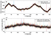 |
Fig. 1. (a) IPPs of the solar LDF (R(i, j)) vs. angular position (Θ(j)) for the roll sequence on July 17, 2019 and for a linear Stokes polarization state (I + Q). All solar limbs at IPP represent measurements at all roll angles. (b) Limb brightness at IPP (B(i, j)) vs. angular position. |
where RNBC(i, j) is the corrected radius, and ⟨R⟩ is the average solar radius calculated over all azimuth angles for each image.
The limb brightness at IPP is not constant; it varies (Figure 1b). Therefore, we developed a method to correct this effect. In Method M1 with brightness correction (BC), this effect is addressed using Eq. (8), as detailed below:
 (8)
(8)
where a is a fitting coefficient that minimizes the squared residuals between the corrected solar radius and a reference fit, and  is the variation of brightness with radius at IPP.
We emphasize that most active regions near the limb are removed from the solar shape before computing the oblateness.
3.1.3. Step 3: Distance correction
To account for the SDO spacecraft’s distance variations from the Sun during each roll sequence, measured solar radii are scaled to a reference distance of 1 astronomical unit (AU).
3.1.4. Step 4: Conversion to Sun-fixed frame
The solar radii data are converted from the HMI telescope CCD frame to the Sun-fixed frame. During the SDO spacecraft’s roll maneuver, it rotates either from north to west (clockwise) or from north to east (counterclockwise), depending on the planned sequence (April, July, or October). The corrected solar radii are processed for the 33 positions taken by the spacecraft (from an initial 0° back to 0°), and the conversion from the CCD frame to the Sun-fixed frame is described by: ΘSun(i, j) = Θ(j)+Roll(i)×11.25°, with 0 ≤ Roll(i)≤32.
3.1.5. Step 5: Solar oblateness calculation
The solar oblateness for each roll sequence and Stokes polarization state on a given date is determined. The corrected solar radii (in the Sun-fixed frame) are fitted using Legendre polynomials (Pl) to calculate the apparent solar shape (r(Θ)), as shown in Eq. (9). This method is commonly used to describe the solar shape. By utilizing this approach, we can determine apparent solar oblateness (Δra) from C2 and C4 (Eq. 10).
 (9)
(9)
and
 (10)
(10)
where Θ is the heliographic colatitude, ⟨r⟩ is the mean solar radius at 1 AU, and  is the Legendre polynomial of degree l shifted to have zero mean (
 ).
).
Regions of the solar limb affected by bright active regions, such as faculae, are excluded from the final fit, as these significantly impact the measurements. However, dark regions like sunspots do not notably affect the results. To further validate and refine the exclusion of active regions, we cross-reference images taken at 393.4 nm (Ca II K) from the Precision Solar Photometric Telescope, which helps identify the solar regions’ activity. Active regions are removed by excluding data points with deviations from the Legendre fit greater than 2 standard deviations (2σ). We then verify the goodness of the fit, indicating how well the data fit the statistical model (an R2 correlation coefficient of 1 indicates a perfect fit), and obtain the uncertainty of the measurements (95% confidence bounds or 2σ).
This methodology ensures accurate determination of solar oblateness using HMI images, accounting for distortions and variations in solar limb profiles.
3.1.6. Polarization dependence
All polarization states were studied. Figure A.1 shows the evolution of the Sun’s shape based on observations from four SDO/HMI roll sequences (October 2010, April 2014, July 2019, October 2023) for a linear Stokes polarization state (I + Q). When spikes are detected, such as the dips near 160° and 340° in the October 2010 observation (Figure A.1), abnormal values are excluded from the dataset. These spikes may be linked to the presence of faculae or to instrumental effects. Removing these outliers helps ensure a more accurate analysis.
When calculating the solar oblateness for different polarization states of the solar light measured by the HMI telescope, we observe consistent results across all states, indicating that the solar oblateness measurements are not affected by the polarization of the observed light. Analysis shows that measurements from different polarization states yield nearly identical results, with correlations exceeding 0.99 across states.
3.2. Solar oblateness from HMI helioseismic inference of internal rotation – Method M2
For Method M2, the determination of solar oblateness involves calculating the J2n gravitational moments. In the case of axial and equatorial symmetry, they appear in the expression of the external solar gravitational potential (ϕout) as in Eq. (11).
![Mathematical equation: $$ \begin{aligned} \phi _{\text{ out}}(r, u) = -\frac{G\mathrm{M} _\odot }{r} \left[ 1 - \sum _{n = 1}^{\infty } \left( \frac{\mathrm{R} _\odot }{r} \right)^{2n} \mathrm{J} _{2n} \mathrm{P} _{2n}(u) \right], \end{aligned} $$](/articles/aa/full_html/2025/01/aa51130-24/aa51130-24-eq14.gif) (11)
(11)
where r represents the distance from the center of the Sun.
The objective is to calculate new values of J2n for a two-dimensional differential rotation Ω(r,u), derived from high-precision helioseismic data obtained with HMI. This data is available on the Joint Science Operations Center (JSOC) website (http://jsoc.stanford.edu/). For Ω(r,u), we use time-averaged two-dimensional rotation rates derived from HMI helioseismic data of full-disk (FDV) dopplergrams, covering the period from April 2010 to the end of 2023. For comparison purposes, we also calculate J2n using rotation rates from MDI data, which are available in the same database for the period between May 1996 and March 2008. This comparison is particularly valuable, as it involves rotation rates derived from an improved recent analysis of FDV MDI helioseismic data (Larson & Schou 2018), which corrects for several geometric effects during spherical harmonic decomposition, as well as other physical effects such as the distortion of eigenfunctions by differential rotation and horizontal displacement at the solar surface. The HMI FDV data, requiring fewer geometric corrections, have been processed in the same way as the MDI FDV data.
In the framework of the hydrodynamic theory of slowly rotating stars (meaning centrifugal acceleration ≪ gravitational acceleration), the quantities describing stellar structure can be expressed as the sum of a perturbed quantity (index 1) and an unperturbed quantity (index 0) describing the spherical state. By decomposing the perturbed state using the basis of P2n Legendre polynomials, the internal gravitational potential (ϕint) can be expressed as in Eq. (12):
 (12)
(12)
The J2n gravitational moments are thus given by the continuity condition of the gravitational potential at the surface (ϕint (R⊙,u) = ϕout(R⊙,u)) as in Eq. (13):
 (13)
(13)
By linearizing the equations of hydrostatic equilibrium and Poisson’s equation, we derive the general form of the equation governing gravitational potential perturbations (Mecheri et al. 2004), as in Eqs. (14)–(16):
 (14)
(14)
with
 (15)
(15)
 (16)
(16)
where the quantities U = 4πρ0r3/Mr and d ln ρ0/d ln r are provided by solar models through the density ρ0 and the mass Mr contained within a sphere of radius r of the Sun.
Using Green’s method described by Pijpers (1998), the differential equation can be transformed into a general integral equation giving ϕ2n at the surface (Mecheri et al. 2004; Mecheri & Meftah 2021), as in Eq. (17):
![Mathematical equation: $$ \begin{aligned} \begin{aligned} \phi _{12n}(\mathrm{R} _\odot )&= -\frac{\mathrm{R} _\odot ^{-2n}}{G\mathrm{M} _\odot } \left[ \frac{r^{2n}}{(2n + 1) \psi _{2n} + r \psi ^{\prime }_{2n}} \right]_{r = \mathrm{R} _\odot } \\&\quad \times \int _{0}^{\mathrm{R} _\odot } r^2 U \left( (V + 2) A_{2n} + r \frac{dA_{2n}}{dr} + B_{2n} \right) \psi _{2n} dr \,, \end{aligned} \end{aligned} $$](/articles/aa/full_html/2025/01/aa51130-24/aa51130-24-eq20.gif) (17)
(17)
where ψ2n(r) is a regular solution at the origin (ψ2n(r) ∝ r2n for r ≃ 0) of Eq. (14) with the right-hand side equal to zero.
Using Eq. (13), we obtain:
![Mathematical equation: $$ \begin{aligned} \begin{aligned} \mathrm{J} _{2n}&= -\left[ \frac{x^{2n}}{(2n + 1) \psi _{2n} + x \psi ^{\prime }_{2n}} \right]_{x = 1} \\&\quad \times \int _{0}^{1} \left( \left( x^2 (U - 4) U \psi _{2n} - x^3 U \psi ^{\prime }_{2n} \right) A_{2n} + x^2 U \psi _{2n} B_{2n} \right) dx \\&= \int _{0}^{1} \int _{-1}^{1} F_{2n}(x, u) \omega (x, u)^2 du dx, \end{aligned} \end{aligned} $$](/articles/aa/full_html/2025/01/aa51130-24/aa51130-24-eq21.gif) (18)
(18)
where F2n represents the integration kernel for the normalized quantities x = r/R⊙ and  ). F2n depends only on the solar model used.
On the other hand, the ρ2n density perturbation is related to ϕ2n through Eq. (19):
 (19)
(19)
The determination of ρ2n at the surface through ϕ2n(R⊙) allows the calculation of the d2n shape parameters, which describe the distortions of constant density contours at the surface (Armstrong & Kuhn 1999), as in Eq. (20):
 (20)
(20)
Consequently, the theoretical solar oblateness Δ⊙ can be determined from the quadrupole term d2 and the hexadecapole term d4 from the method based on HMI helioseismic inference of internal rotation, as in Eq. (21):
 (21)
(21)
This method enables the calculation of the quantities J2n and d2n (which are comparable to the C2n values determined using Method M1), as well as the resulting solar oblateness Δ⊙ using all rotation data over solar cycles. This approach aims to explore potential temporal variations, whether or not they correlate with solar magnetic activity.
4. Results and discussion
We analyzed twenty-three SDO/HMI roll sequences conducted between October 2010 and November 2023. The SDO satellite orbits at an altitude of 35 789 km, positioned at 102° West longitude with an inclination of 28.5°, performing solar oblateness measurements twice a year. Figure 2 illustrates the distribution of these roll maneuvers across solar cycles 24 and 25, showing the variations in sunspot activity.
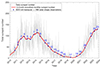 |
Fig. 2. Daily total sunspot number (gray) and 13-month smoothed monthly sunspot number (red) from 2010 to 2024. Each roll sequence used to determine solar oblateness is represented by a blue dot, numbered sequentially from 1 to 23. |
4.1. Solar equator-to-pole radius difference results – ΔR
The solar equator-to-pole radius difference was measured both without brightness correction (NBC) and with brightness correction (BC) at the inflection point position of the solar limb-darkening function, using the Method M1 detailed in Section 3.1. Figure 3 shows the evolution of the equator-to-pole radius difference over time, derived from solar limb shape observations using Method M1 (NBC) for two polarization states: linear (I + Q) and (I − V). We focus on only two polarization states (Figure 3) to demonstrate the strong consistency observed across all six.
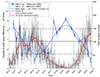 |
Fig. 3. Evolution of ΔR over time, obtained through solar limb shape observations (Method M1) with no brightness correction (NBC) for two polarization states: I + Q and I − V. |
For instance, the I + Q and I − V polarization states exhibit exceptionally high linear correlations, with coefficients of 0.9971 and up to 0.9900 when considering all six polarization states. This indicates a very high similarity among the polarization states. We can conclude that the variations observed in one signal are almost entirely reflected in the others, highlighting an extreme level of coherence and redundancy in the observations. Consequently, the influence of polarization state on the measurements is minimal.
The average value of ΔR across both polarization states is 6.84 ± 1.32 mas (1σ) for the entire time-series. Throughout the 2010–2023 period, potential instrumental effects, possibly linked to temperature variations of the HMI instrument, can influence the calculated solar equator-to-pole radius difference. At the beginning of the SDO mission in 2010, the raw solar radius measurements from the HMI instrument were affected by an unoptimized thermal control system, which operated the thermal heaters at a constant duty cycle. Following a modification in 2013 to stabilize the optical bench temperature at 20° through adjusted heater duty cycles, this influence becomes less evident after 2014, as the HMI thermal control modifications ensured a more consistent and stable temperature. Additionally, we observed a gradual long-term temperature increase in the front window, attributed to aging effects from radiation darkening. This process causes an increase in solar flux absorption and a corresponding decrease in transmission through the window, with transmission decreasing by approximately 4% annually in the initial observation years. These effects could contribute to variations in the ΔR time-series, reflecting the complex interplay of instrumental aging and temperature stability over time.
There may therefore be an instrumental impact on solar equator-to-pole radius difference (Method M1 (NBC)). Nevertheless, we proceed to examine the relationship between ΔR and solar activity. To determine whether the equator-to-pole radius difference is in phase, out of phase, or indeterminate with respect to solar activity (total sunspot number), we applied a one-term Fourier series to the calculated ΔR values (Figure 3) derived from each HMI roll sequence, excluding potential instrumental effects. The fitted model for ΔR over time (t in days, starting from October 10, 2010), is given by: ΔR(t) = 7.000 ± 0.435 + (1.267 ± 0.710) × cos(0.00178 ± 0.00026 t) − (0.8433 ± 0.9877) × sin(0.00178 ± 0.00026 t) with 95% confidence bounds for each parameter. The primary oscillatory behavior of ΔR reveals a period of approximately 9.9 years, with an uncertainty of ±1.4 years at the 95% confidence level. The fitted model serves as the basis for the correlation comparison with solar activity, highlighting the strong anti-phase relationship (Pearson’s correlation of −0.8) between ΔR and solar cycles. This result is interesting but questionable because some values of ΔR(t) (in mas) are less than 7.8 mas (ΔRSurf). Indeed, ΔR below 7.8 mas would contradict well-established physical models and observational evidence, suggesting that any values below this threshold may be the result of instrumental errors or data processing issues rather than reflecting a true physical state of the Sun. Nevertheless, the observed anti-phase between ΔR and solar activity may exist and be amplified by instrumental effects.
In addition to these results, we have obtained further findings using Method M1 (BC), which specifically addresses variations in limb brightness at the inflection point position. Figure 4 illustrates the evolution of the equator-to-pole radius difference over time, as obtained through solar limb shape observations using Method M1 (BC) for two polarization states: linear (I + Q) and (I − V). The linear correlation between the I + Q and I − V polarization states is 0.9931, with correlations exceeding 0.9900 across all six polarization states. As with Method M1 (NBC), the influence of polarization state on the measurements is negligible.
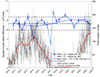 |
Fig. 4. Evolution of ΔR over time, obtained through solar limb shape observations (Method M1) with brightness correction (BC) for two polarization states: I + Q and I − V. |
Based on Method M1 (BC), we calculated an average ΔR value of 8.66 ± 0.69 mas (1σ) for the entire time series. The one-term Fourier series fitted to the ΔR values suggests an anti-phase relationship with solar activity; however, this relationship is not statistically significant, as the Pearson’s R2 correlation coefficient is below 0.1. This suggests that the model does not adequately capture the observed variability, and thus the interpretation of this anti-phase relationship with solar activity lacks a solid foundation.
The solar equator-to-pole radius difference was also obtained using Method M2, which is based on HMI helioseismic rotational rates derived from high-resolution data on internal solar rotation, as detailed in Section 3.2. Figure 5 illustrates the temporal evolution. The uncertainty for each measurement is on the order of ±0.01 mas at 1σ (see Appendix D). The average ΔR across the time-series is 8.05 ± 0.02 mas (1σ), with a peak-to-peak variation from 8.02 to 8.09 mas.
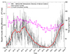 |
Fig. 5. ΔR time evolution, as determined through helioseismology (Method M2), which exhibits slight variations during sunspot cycles 24 and 25 (∼0.05 mas), with peak-to-peak values ranging from 8.02 to 8.09 mas. |
We also examined the relationship between ΔR, as calculated using Method M2, and solar activity to determine whether they are in phase or not. The fitted model for ΔR over time (t in days, starting from October 10, 2010), is given by: ΔR(t) = 8.052 ± 0.003 + (0.0048 ± 0.0061)×cos(0.00128 ± 0.00012 t) + (0.02023 ± 0.00416)×sin(0.00128 ± 0.00012 t) with 95% confidence bounds for each parameter. The period is approximately 13.5 ± 1.2 years (95% confidence bounds). The fitted model provides a foundation for comparing correlation with solar activity, underscoring a significant phase relationship (Pearson’s correlation coefficient of 0.69) between ΔR (Method M2) and the solar cycles. The variation in ΔR from 2010 to 2023, based on Method M2, is 0.050 ± 0.007 mas (1σ).
4.2. Solar oblateness results – Δ⊙
The solar oblateness was determined using Method M1 (HMI solar disk images and limb observations), incorporating a brightness intensity correction to mitigate potential distortions from instrumental effects, such as variations in the telescope’s PSF. This approach represents the most accurate method for the absolute determination of solar oblateness. The resulting average solar oblateness during the period 2010–2023 has been calculated as 9.02 (±0.72) × 10−6, equivalent to a ΔR solar radius difference of 8.66 ± 0.69 mas (6.28 ± 0.50 kilometers) representing the best attempt so far from limb observations, where C2 and C4 are respectively equal to ( − 6.11 ± 0.55)×10−6 and (2.37 ± 2.99)×10−7 (Figures B.1 and B.2). Based on Method M1 with brightness correction, it is difficult to conclude regarding the correlation between C2 and C4 with the solar activity. However, when there is no brightness correction, the quadrupole coefficient (C2) evolves in phase with solar activity, while it is more difficult to draw conclusions regarding the hexadecapole coefficient (C4). Results obtained using Method M1 (NBC and BC) are provided in Appendix C.
Additionally, the solar oblateness was determined using Method M2 (HMI helioseismic inference of internal rotation). In this approach, we calculated the values of J2n and, subsequently, determine the solar oblateness. We achieved this by utilizing two-dimensional rotation rates derived from high-resolution data collected by SDO/HMI from 2010 to 2023. We developed a general integral equation that establishes the relationship between J2n and the internal density and rotation of the Sun. This equation is based on the structural equations that govern the equilibrium of slowly rotating stars (Mecheri & Meftah 2021). From HMI helioseismic inference of internal rotation, we have determined the quadrupole coefficient d2 to be (−5.85 ± 0.01)×10−6, and for the d4 hexadecapole coefficient, the value is (6.07 ± 0.11) × 10−7. This leads to an helioseismic solar oblateness of 8.40 (±0.02)×10−6. About d2 and d4, they are in phase with solar activity.
4.3. Discussion
HMI solar oblateness was determined using two methods (solar limb shape observations and helioseismic inference of internal rotation). Results from both techniques are consistent and confirm that the Sun is rotating as expected, addressing specific queries (Gough 2012). The average solar equator-to-pole radius difference obtained is 8.66 ± 0.69 mas for the method based on solar limb shape observations, and 8.05 ± 0.14 mas for the helioseismology-based method, indicating that the oblateness is not as small as suggested by Kuhn et al. (2012). Figures 4 and 5 show how solar oblateness changes over time using these two methods (Method M1 with brightness correction and Method M2 based on helioseismic data). For both methods, we observe that the solar oblateness has stayed roughly constant over the 13 years of observation. However, we note that the solar oblateness determined from the solar limb shape seems to be in anti-phase with solar activity with no evidence of temporal variability in the Sun’s shape and no evidence that these solar oblateness measurements were temporally affected by near-surface (dynamo and/or interior) magnetic fields. Conversely, the solar oblateness determined from helioseismology shows an evident slight variation in phase with solar activity. A variable solar shape either requires an enigmatically large perturbation of the interior mass and/or rotation distribution or suggest a misinterpretation of the measured solar shape, potentially caused by factors such as photospheric magnetic contamination.
Helioseismology reveals that the disturbances in the Sun’s spherical symmetry are localized in its outer layers (subsurface layers). These surface disturbances are closely correlated with solar activity. Although standard helioseismic methods, including surface gravity modes (f-modes), allow examination of the Sun’s interior rotation very close to the surface (Barekat et al. 2014), these methods may still have reduced sensitivity to rotation in the outermost layers. Inversions incorporating f-modes, such as those used in HMI data, provide insights into rotation up to nearly the visible surface, or close to 1.00 R⊙, where the C2n coefficients are calculated. Additionally, other observational techniques contribute to our understanding of surface rotation beyond the results from helioseismic data alone.
Solar limb observations are made extremely close to the surface, effectively at a radius of approximately 1.00 R⊙ with minimal deviation, typically within 0.001 R⊙. The divergence between our results and other findings might stem from analyzing rotational behavior at slightly different radii below the surface. Such differences in behavior have been previously discussed by Emilio et al. (2007) and Lefebvre et al. (2007), suggesting the potential for non-homologous expansion within the Sun’s internal layers. This was further supported by numerical simulations conducted by Sofia & Li (2005). On the other hand, asphericities are caused by rotation and possibly by the presence of an internal magnetic field or any other factor that could break the Sun’s spherical symmetry. Therefore, helioseismology accounts for all these effects when calculating asphericities. Is this also true for solar limb measurements?
Do the C2 and C4 coefficients only reflect surface effects (attributed to the impact of rotation on outer layers), or do they also indicate deeper deformations possibly caused by an internal magnetic field? In calculations using the helioseismic method, it is certain that the shape parameters derived are due to differential rotation, as the hydrodynamic model used does not consider a magnetic field but does include a differential rotation profile provided by helioseismic data from the HMI instrument. The observed solar cycle variations and the indirect effect of differential rotation’s dependence on the solar cycle, which has been long detected, are important. This dependence of rotation, in turn, stems from the observed correlation of pulsation modes with magnetic activity. As example, the frequencies of the p-modes (solar acoustic oscillations) correlate with solar activity. Specifically, during periods of higher solar activity, such as during solar maximum, the frequencies of p-modes tend to increase, while they decrease during solar minimum.
The contribution to the quadrupole moment (J2 = (2.21 ± 0.01)×10−7 in our HMI helioseismic analysis vs. (5.97 ± 4.79)×10−7 from solar limb shape observations) primarily originates from the Sun’s inner region, where the integration kernel reaches its maximum value around 0.71 R⊙, corresponding to the base of the convection zone. In contrast, the contribution to the higher-order moments predominantly comes from the outer layers, where the corresponding integration kernel exhibits significant radial and latitudinal variations. This makes them highly sensitive to differential rotation in the convective zone, and consequently, to the observed temporal variations in the latitudinal part of the rotation, which shows correlations with solar activity. Hence, the correlations found for J4 ((4.24 ± 0.06) × 10−9 in our HMI helioseismic analysis), J6, J8, and J10 with the solar cycle, either in phase or anti-phase. J2, which is particularly sensitive to the rotation of the inner part in the radiative zone (where rotational dynamics play a key role in shaping the Sun’s gravitational field), exhibits minimal temporal variation. This is because the rotation of the inner layers remains relatively constant, as revealed by observations. The J2n and C2n coefficients provide important insights into the internal physical mechanisms disrupting the spherical symmetry of stars. If a correlation with solar activity exists, these parameters are crucial for constraining solar dynamo models and for predicting the evolution of solar cycles.
5. Conclusions
The determination of solar oblateness using data from the Helioseismic Magnetic Imager aboard NASA’s Solar Dynamics Observatory offers critical insights into the Sun’s internal structure and dynamics. Over the 13–year observation period from 2010 to end of 2023, we used two methods to measure solar oblateness: direct limb shape observations and helioseismic inference of internal rotation.
Our findings reveal that the average solar oblateness, determined through direct solar limb shape observations, is 9.02 × 10⁻⁶ (equivalent to a solar radius difference of 8.66 ± 0.69 mas or 6.28 ± 0.50 kilometers). This value is unaffected by brightness contamination from sunspots and magnetically induced excess emission. Furthermore, the solar oblateness derived from direct solar limb shape observations using various HMI Stokes polarization states (Q, U and V) shows no significant difference. Interestingly, the HMI time-series of oblateness derived from direct solar limb shape observations appears to be in anti-phase with sunspot cycle (Schwabe cycles 24 and 25). Our HMI solar limb shape observations using Method M1, without brightness correction (NBC), reveal a moderately strong correlation between solar activity and solar oblateness.
Using helioseismic data to derive the internal differential rotation rates, we calculated the J2n gravitational moments, resulting in a solar oblateness of 8.40 × 10⁻⁶. The quadrupole moment J2 calculated from HMI helioseismic data, at 2.21 × 10⁻⁷, aligns closely with values derived from other observational data, such as Messenger’s telemetry, which measured J2 = 2.25 × 10⁻⁷ (Genova et al. 2018). This agreement reinforces the accuracy and reliability of our results. The determination from helioseismic inference of internal rotation indicates that the solar oblateness varies slightly in phase with solar activity, highlighting the sensitivity of helioseismic methods to changes in the Sun’s internal rotation and mass distribution. This method seems to be much more suitable for determining solar oblateness over time.
Acknowledgments
This research has been conducted with the support of Académie Spatiale Île de France, Stanford University, the University of Hawai’i System, and the Programme National Soleil Terre (PNST, France) of CNRS/INSU (France) co-funded by Centre National d’Études Spatiales (CNES, France) and Commissariat à l’énergie atomique (CEA, France). We acknowledge the courtesy of NASA/SDO and the HMI science teams for providing access to HMI data. We would particularly like to express our special thanks to Phil Scherrer (Stanford University), Jeff Kuhn (University of Hawai’i System), Rock Bush (Stanford University), and Kader Amsif (CNES). We also thank the anonymous referee for their constructive feedback. Lastly, this study relies on sunspot number data obtained from the Solar Influences Data Analysis Center (SIDC) at the Royal Observatory of Belgium, Brussels.
References
- Antia, H. M., Chitre, S. M., & Gough, D. O. 2008, A&A, 477, 657 [NASA ADS] [CrossRef] [EDP Sciences] [Google Scholar]
- Armstrong, J., & Kuhn, J. R. 1999, ApJ, 525, 533 [NASA ADS] [CrossRef] [Google Scholar]
- Barekat, A., Schou, J., & Gizon, L. 2014, A&A, 570, L12 [NASA ADS] [CrossRef] [EDP Sciences] [Google Scholar]
- Chao, B. F. 2006, C. R. Geosci., 338, 1123 [NASA ADS] [CrossRef] [Google Scholar]
- Damiani, C., Rozelot, J. P., Lefebvre, S., Kilcik, A., & Kosovichev, A. G. 2011, J. Atmos. Sol. Terr. Phys., 73, 241 [NASA ADS] [CrossRef] [Google Scholar]
- Dicke, R. H. 1970, ApJ, 159, 1 [NASA ADS] [CrossRef] [Google Scholar]
- Dicke, R. H., & Goldenberg, H. M. 1967, Phys. Rev. Lett., 18, 313 [NASA ADS] [CrossRef] [Google Scholar]
- Dicke, R. H., Kuhn, J. R., & Libbrecht, K. G. 1987, ApJ, 318, 451 [NASA ADS] [CrossRef] [Google Scholar]
- Egidi, A., Caccin, B., Sofia, S., et al. 2006, Sol. Phys., 235, 407 [NASA ADS] [CrossRef] [Google Scholar]
- Einstein, A. 1916, Ann. Phys., 354, 769 [Google Scholar]
- Emilio, M., Bush, R. I., Kuhn, J., & Scherrer, P. 2007, ApJ, 660, L161 [NASA ADS] [CrossRef] [Google Scholar]
- Fivian, M. D., Hudson, H. S., Lin, R. P., & Zahid, H. J. 2008, Science, 322, 560 [NASA ADS] [CrossRef] [Google Scholar]
- Genova, A., Mazarico, E., Goossens, S., et al. 2018, Nat. Commun., 9, 289 [NASA ADS] [CrossRef] [Google Scholar]
- Gough, D. 2012, Science, 337, 1611 [NASA ADS] [CrossRef] [Google Scholar]
- Irbah, A., Meftah, M., Hauchecorne, A., et al. 2014, ApJ, 785, 89 [NASA ADS] [CrossRef] [Google Scholar]
- Irbah, A., Mecheri, R., Damé, L., & Djafer, D. 2019, ApJ, 875, L26 [NASA ADS] [CrossRef] [Google Scholar]
- Kuhn, J. R., Bush, R., Emilio, M., & Scholl, I. F. 2012, Science, 337, 1638 [NASA ADS] [CrossRef] [Google Scholar]
- Larson, T. P., & Schou, J. 2018, Sol. Phys., 293, 29 [Google Scholar]
- Le Verrier, U. J. 1859, Théorie du mouvement de Mercure. Annales de l’Observatoire de Paris, 5, 1 [Google Scholar]
- Lefebvre, S., Kosovichev, A. G., & Rozelot, J. P. 2007, ApJ, 658, L135 [NASA ADS] [CrossRef] [Google Scholar]
- Mecheri, R., & Meftah, M. 2021, MNRAS, 506, 2671 [NASA ADS] [CrossRef] [Google Scholar]
- Mecheri, R., Abdelatif, T., Irbah, A., Provost, J., & Berthomieu, G. 2004, Sol. Phys., 222, 191 [NASA ADS] [CrossRef] [Google Scholar]
- Meftah, M., Irbah, A., Hauchecorne, A., et al. 2015, Sol. Phys., 290, 673 [NASA ADS] [CrossRef] [Google Scholar]
- Meftah, M., Hauchecorne, A., Bush, R. I., & Irbah, A. 2016, Adv. Space Res., 58, 1425 [NASA ADS] [CrossRef] [Google Scholar]
- Meftah, M., Corbard, T., Hauchecorne, A., et al. 2018, A&A, 616, A64 [NASA ADS] [CrossRef] [EDP Sciences] [Google Scholar]
- Misner, C. W., Thorne, K. S., & Wheeler, J. A. 1973, Gravitation (San Francisco: W. H. Freeman and Company) [Google Scholar]
- Newcomb, S. 1895, AJ, 14, 185 [NASA ADS] [CrossRef] [Google Scholar]
- Paterno, L., Sofia, S., & di Mauro, M. P. 1996, A&A, 314, 940 [NASA ADS] [Google Scholar]
- Pijpers, F. P. 1998, MNRAS, 297, L76 [NASA ADS] [CrossRef] [Google Scholar]
- Rozelot, J. P., Damiani, C., & Pireaux, S. 2009, ApJ, 703, 1791 [NASA ADS] [CrossRef] [Google Scholar]
- Scherrer, P. H., Schou, J., Bush, R. I., et al. 2012, Sol. Phys., 275, 207 [Google Scholar]
- Schou, J., Scherrer, P. H., Bush, R. I., et al. 2012, Sol. Phys., 275, 229 [Google Scholar]
- Sofia, S., & Li, L. H. 2005, Mem. Soc. Astron. It., 76, 768 [NASA ADS] [Google Scholar]
Appendix A: Sun’s shape through SDO/HMI observations at 617.334 nm – Method M1.
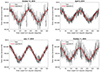 |
Fig. A.1. Evolution of the Sun’s shape based on observations from four SDO/HMI roll sequences – for a linear Stokes polarization state (I+Q). The solar limb shape is approximated using low-order Legendre polynomials fit. The October 12, 2010 plot shows very large dips around 160 and 340 degrees. These values have been excluded from the analysis, and similar anomalies (due to sunspots or instrumental effects) in other datasets have been carefully filtered out to prevent them from impacting the overall results. The spiky periodicities observed, particularly on October 11, 2023, could be attributed to instrumental effects or minor issues with the spacecraft’s pointing accuracy. These periodic spikes may result from slight pointing deviations during data acquisition, which can impact measurement consistency. Instrument-related factors, such as sensor noise or calibration shifts, might also play a role. While these explanations are plausible, they highlight the need to carefully consider potential spacecraft or instrument artifacts in the analysis. |
Appendix B: Temporal evolution of the Sun’s quadrupole (C2) and hexadecapole (C4) coefficients from 2010 to 2023 through SDO/HMI observations at 617.334 nm – Method M1.
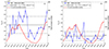 |
Fig. B.1. (a) Evolution of C2 over time, obtained from HMI solar limb shape observations using Method M1 without brightness correction (NBC) for a linear polarization state (I+Q). (b) Evolution of C2 over time, obtained from HMI solar limb shape observations using Method M1 with brightness correction (BC) for the same linear polarization state (I+Q). |
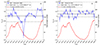 |
Fig. B.2. (a) Evolution of C4 over time, obtained from HMI solar limb shape observations using Method M1 without brightness correction (NBC) for a linear polarization state (I+Q). (b) Evolution of C4 over time, obtained from HMI solar limb shape observations using Method M1 with brightness correction (BC) for the same linear polarization state (I+Q). |
Appendix C: Results for two polarization states of the SDO/HMI telescope – Method M1.
Results obtained using Method M1 (NBC) for I+Q linear polarization at 0 deg – at 617.334 nm.
Results obtained using Method M1 (BC) for I+Q linear polarization at 0 deg – at 617.334 nm.
Results obtained using Method M1 (NBC) for I-V right circular polarization – at 617.334 nm.
Results obtained using Method M1 (BC) for I-V right circular polarization – at 617.334 nm.
Appendix D: Results obtained from HMI helioseismic inference of internal rotation – Method M2.
Results obtained using Method M2 – at 617.334 nm.
All Tables
Results obtained using Method M1 (NBC) for I+Q linear polarization at 0 deg – at 617.334 nm.
Results obtained using Method M1 (BC) for I+Q linear polarization at 0 deg – at 617.334 nm.
Results obtained using Method M1 (NBC) for I-V right circular polarization – at 617.334 nm.
Results obtained using Method M1 (BC) for I-V right circular polarization – at 617.334 nm.
All Figures
|
Fig. 1. (a) IPPs of the solar LDF (R(i, j)) vs. angular position (Θ(j)) for the roll sequence on July 17, 2019 and for a linear Stokes polarization state (I + Q). All solar limbs at IPP represent measurements at all roll angles. (b) Limb brightness at IPP (B(i, j)) vs. angular position. |
| In the text | |
|
Fig. 2. Daily total sunspot number (gray) and 13-month smoothed monthly sunspot number (red) from 2010 to 2024. Each roll sequence used to determine solar oblateness is represented by a blue dot, numbered sequentially from 1 to 23. |
| In the text | |
|
Fig. 3. Evolution of ΔR over time, obtained through solar limb shape observations (Method M1) with no brightness correction (NBC) for two polarization states: I + Q and I − V. |
| In the text | |
|
Fig. 4. Evolution of ΔR over time, obtained through solar limb shape observations (Method M1) with brightness correction (BC) for two polarization states: I + Q and I − V. |
| In the text | |
|
Fig. 5. ΔR time evolution, as determined through helioseismology (Method M2), which exhibits slight variations during sunspot cycles 24 and 25 (∼0.05 mas), with peak-to-peak values ranging from 8.02 to 8.09 mas. |
| In the text | |
|
Fig. A.1. Evolution of the Sun’s shape based on observations from four SDO/HMI roll sequences – for a linear Stokes polarization state (I+Q). The solar limb shape is approximated using low-order Legendre polynomials fit. The October 12, 2010 plot shows very large dips around 160 and 340 degrees. These values have been excluded from the analysis, and similar anomalies (due to sunspots or instrumental effects) in other datasets have been carefully filtered out to prevent them from impacting the overall results. The spiky periodicities observed, particularly on October 11, 2023, could be attributed to instrumental effects or minor issues with the spacecraft’s pointing accuracy. These periodic spikes may result from slight pointing deviations during data acquisition, which can impact measurement consistency. Instrument-related factors, such as sensor noise or calibration shifts, might also play a role. While these explanations are plausible, they highlight the need to carefully consider potential spacecraft or instrument artifacts in the analysis. |
| In the text | |
|
Fig. B.1. (a) Evolution of C2 over time, obtained from HMI solar limb shape observations using Method M1 without brightness correction (NBC) for a linear polarization state (I+Q). (b) Evolution of C2 over time, obtained from HMI solar limb shape observations using Method M1 with brightness correction (BC) for the same linear polarization state (I+Q). |
| In the text | |
|
Fig. B.2. (a) Evolution of C4 over time, obtained from HMI solar limb shape observations using Method M1 without brightness correction (NBC) for a linear polarization state (I+Q). (b) Evolution of C4 over time, obtained from HMI solar limb shape observations using Method M1 with brightness correction (BC) for the same linear polarization state (I+Q). |
| In the text | |
Current usage metrics show cumulative count of Article Views (full-text article views including HTML views, PDF and ePub downloads, according to the available data) and Abstracts Views on Vision4Press platform.
Data correspond to usage on the plateform after 2015. The current usage metrics is available 48-96 hours after online publication and is updated daily on week days.
Initial download of the metrics may take a while.