| Issue |
A&A
Volume 693, January 2025
|
|
|---|---|---|
| Article Number | A132 | |
| Number of page(s) | 10 | |
| Section | Planets, planetary systems, and small bodies | |
| DOI | https://doi.org/10.1051/0004-6361/202450598 | |
| Published online | 10 January 2025 | |
A new pathway to SO2
Revealing the NUV driven sulfur chemistry in hot gas giants
1
Anton Pannekoek Institute for Astronomy, University of Amsterdam,
1090GE
Amsterdam,
The Netherlands
2
Department of Earth and Planetary Sciences, University of California,
Riverside,
CA,
USA
3
SRON Netherlands Institute for Space Research,
Niels Bohrweg 4,
2333
CA
Leiden,
The Netherlands
4
Department of Astrophysics/IMAPP, Radboud University Nijmegen,
PO Box 9010,
6500
GL
Nijmegen,
The Netherlands
5
Institute of Astronomy, KU Leuven,
Celestijnenlaan 200D,
3001
Leuven,
Belgium
★ Corresponding author; wiebedg@gmail.com
Received:
3
May
2024
Accepted:
4
November
2024
Context. Photochemistry is a key process that drives planetary atmospheres away from local thermodynamic equilibrium. Recent observations of the H2 dominated atmospheres of hot gas giants have detected SO2 as one of the major products of this process.
Aims. We investigated which chemical pathways lead to the formation of SO2 in an atmosphere, and we investigated which part of the flux from the host star is necessary to initiate SO2 production.
Methods. We used the publicly available S–N–C–H–O photochemical network in the VULCAN chemical kinetics code to compute the disequilibrium chemistry of an exoplanetary atmosphere.
Results. We find that there are two distinct chemical pathways that lead to the formation of SO2. The formation of SO2 at higher pressures is initiated by stellar flux >200 nm, whereas the formation of SO2 at lower pressures is initiated by stellar flux <200 nm. In deeper layers of the atmosphere, OH is provided by the hydrogen abstraction of H2O, and sulfur is provided by the photodissociation of SH and S2, which leads to a positive feedback cycle that liberates sulfur from the stable H2S molecule. In the upper layers of the atmosphere, OH is provided by the photodissociation of H2O, and sulfur can be liberated from H2S either by the photodissociation of SH and S2, or by the hydrogen abstraction of SH.
Conclusions. We conclude that the stellar flux in the 200–350 nm wavelength range as well as the ratio of near-UV to UV radiation are important parameters determining the observability of SO2. In addition, we find that there is a diversity of chemical pathways to the formation of SO2. This is crucial for the interpretation of SO2 detections and derived elemental abundance ratios, and for overall metallicities.
Key words: planets and satellites: atmospheres / planets and satellites: composition / planets and satellites: gaseous planets / planet–star interactions
© The Authors 2025
 Open Access article, published by EDP Sciences, under the terms of the Creative Commons Attribution License (https://creativecommons.org/licenses/by/4.0), which permits unrestricted use, distribution, and reproduction in any medium, provided the original work is properly cited.
This article is published in open access under the Subscribe to Open model. Subscribe to A&A to support open access publication.
1 Introduction
Giant planets on short orbital periods represent an important and well-studied group of exoplanets, due to observational biases that make it relatively easy to detect these planets and probe their atmospheres. A major challenge currently facing the field of exoplanets is to understand their formation and evolution, so that we can place them in the wider context of the planetary systems to which they belong (Boley 2009; Rafikov 2005).
The abundances of elements such as C, N, O, and S in the atmosphere provide a window into a planet’s evolutionary history (Turrini et al. 2021). Telescopes such as Hubble and Spitzer have laid down the groundwork for characterizing the chemical composition of giant planet atmospheres (Madhusudhan 2019), and recently, with the advent of the James Webb Space Telescope (JWST), our capabilities of identifying chemical species in an exoplanet’s atmosphere have increased markedly. Of particular importance among the newly detected molecules is sulfur dioxide (SO2), which has been detected by JWST in the atmospheres of WASP-39b (Rustamkulov et al. 2023) and WASP-107b (Dyrek et al. 2024).
The presence of SO2 in the atmosphere of a hot gas giant is important for two reasons. First, the production of SO2 is an outcome of photochemistry, as shown by Tsai et al. (2023a), which marks the first time that the effects of this physical process have been observed directly in an exoplanetary atmosphere. Second, its detectability depends strongly on the C/O ratio and the metal- licity of the atmosphere (Polman et al. 2023; Dyrek et al. 2024), making it a tracer of two key parameters to constrain a planet’s evolutionary history (Öberg et al. 2011).
Modeling the chemistry in exoplanet atmospheres is challenging due to the need for accurate measurements of reaction rates over a wide range of pressures and temperatures to construct a chemical network (Chubb et al. 2024). For this reason, thermo-photochemical models initially focused mainly on H, C, N, and O chemistry. These models were constructed and applied to hot Jupiters by Moses et al. (2011) and Venot et al. (2012), among others. A substantial effort has been undertaken in recent years to incorporate sulfur chemistry into chemical kinetics models. The first inclusion of sulfur in a chemical kinetics model of a hot Jupiter was conducted by Zahnle et al. (2009), who used it to study the atmospheric heating properties of hot Jupiters. In recent years, model complexity has greatly increased due to the expansion of photochemical networks and measurements of the reaction rates of additional chemical reactions. Sulfur chemistry is now included in 1D photochemical codes such as LEVI (Hobbs et al. 2021), which was applied to atmospheres in the 1000–1400 K range and used to investigate the mixing ratios of SH, H2S, and S2 and their effects on the major N and C bearing molecules; VULCAN (Tsai et al. 2021), which was used to study the impact of sulfur on photochemical haze precursors; and ARGO (Rimmer et al. 2021), which was applied to the atmosphere of Venus with clouds included to explain the SO2 depletion in the upper layer of the atmosphere.
The recent observations of SO2 in gas giant atmospheres and the availability of S–N–C–H–O photochemical networks call for an in-depth investigation of the chemical pathways responsible for SO2 formation, and of the role of the stellar spectral energy distribution (SED). For this paper we analyzed the chemical pathways that lead to the formation of SO2, building on previous work in this direction by Tsai et al. (2023a). We expanded on their work by examining which parts of the stellar SED play a part in the production of SO2, and by examining its dependence on the surface gravity and atmospheric temperature. This study provides a deeper understanding of the photochemistry occurring in the atmospheres of gas giants, which will be essential in interpreting the recent and forthcoming observations targeting hot Jupiters.
In Sect. 2 we describe the method we used to calculate the chemical composition of the atmosphere from an initial set of elemental abundances. We also describe the method we used to compute transmission spectra from the chemical composition. In Sect. 3, we define our fiducial model, and in Sect. 4 we describe our results. In Sect. 5, we discuss our findings and highlight the implications for future observations. In Sect. 6, we provide a summary of our results.
2 Methods
2.1 Chemical composition
We used the photochemical kinetics code VULCAN to calculate the chemical structure of the atmosphere (Tsai et al. 2021), using a parameterized temperature-pressure (TP) profile and evolving the chemical abundances until they reached a state of equilibrium. We used the S–N–C–H–O thermo-photochemical network that is included in the VULCAN distribution. This network consists of 89 species, including 19 S-bearing species; 1030 thermochemical reactions, including forward and reverse reactions; and 60 photodissociation reactions. VULCAN solves the following set of Eulerian continuity equations:
 (1)
(1)
Here ni is the number density in cm−3 of species i; t is the time; Pi and Li are the production and loss rates in cm−3 s−1; and ϕi is the vertical transport flux in cm−2 s−1.
We used 150 vertical atmospheric layers, as is recommended for VULCAN, log-distributed from 103 to 10−8 bar. For the convergence parameters we used the standard values δ = 0.01, which denotes the absolute change in abundances, and є = 10−4, which denotes the time derivative of the abundances, as recommended by Tsai et al. (2017).
We set the elemental abundances by choosing a value for the metallicity and C/O ratio for our atmosphere. We started from the solar elemental abundances determined by Asplund et al. (2009), and we subsequently scaled the carbon abundance to obtain the required C/O ratio. We then scaled the hydrogen and helium abundances to obtain the desired metallicity, where we left the H/He ratio unchanged. We assumed a constant Kzz of 109 cm2/s throughout the atmosphere.
2.2 Temperature-pressure profile
We used a parameterized TP profile, which we took from the approximation derived by Guillot (2010), who modeled the atmosphere with a double-gray approximation. This approximation is described by the following equation:
![$\matrix{ {{T^4} = {{3T_{{\rm{int}}}^4} \over 4}\left[ {{2 \over 3} + \tau } \right] + {{3T_{{\rm{irr}}}^4} \over 4}f\left[ {{2 \over 3} + {1 \over {\gamma \sqrt 3 }}} \right.} \cr {\left. { + \left( {{\gamma \over {\sqrt 3 }} - {1 \over {\gamma \sqrt 3 }}} \right)\exp ( - \gamma \tau \sqrt 3 )} \right].} \cr } $](/articles/aa/full_html/2025/01/aa50598-24/aa50598-24-eq2.png) (2)
(2)
Here, Tint is the internal temperature of the planet; τ is the optical depth to thermal radiation; Tirr is the stellar effective temperature scaled to the distance of the planet by the formula  , where D is the distance to the star; f scales the redistribution of heat around the planet; and γ is the ratio of visible to thermal opacity in the atmosphere, as defined by
  , where κv is the atmospheric opacity to visual radiation, and κth the opacity to infrared radiation. We calculated the pressure assuming constant gravity and hydrostatic equilibrium, according to the equation
  .
.
2.3 Transmission spectrum
To generate transmission spectra from the chemical composition and TP profile, we used the Artful modeling Code for exoplanet Science (ARCiS) (Ormel & Min 2019; Min, Michiel et al. 2020). Within ARCiS, we used the option to set the chemical composition of the atmosphere with the values obtained in VULCAN, and we used a spectral resolution of R=150. We included collision induced absorption and the effect of Rayleigh scattering. Opacity data is available for 27 of the 89 species included in the VULCAN S–N–C–H–O network: SO2, SH, OH, O2, O, NS, NO2, NO, NH3, NH, N2O, N2, HCN, H2S, H2O2, H2O, H2CO, H2, CS, CO2, CO, CN, CH4, CH, C2H4, C2H2, C2. This includes all of the most abundant species, with the exception of SO, which was not included in ARCiS at the time of writing this paper. The opacity of SO is now available and deserves to be considered in future work since SO is expected to be the parent molecule to produce SO2 (Tsai et al. 2023a). However, SO’s opacity overlaps with SO2 in the NIRSpec and MIRI wavelength ranges, making it challenging to detect this molecule.
ARCiS uses line lists from the ExoMol project (Tennyson et al. 2016), and the HITRAN (Gordon et al. 2017) and HITEMP (Rothman et al. 2010) databases. ARCiS uses correlated-k tables, which provide an inexpensive way to incorporate molecular lines into radiative transfer calculations (Lacis & Oinas 1991; Goody et al. 1989). The k-tables (at R=1000 for λ = 0.3–50 µm) were taken from Chubb et al. (2021), who computed them using the Exocross program (Yurchenko et al. 2018).
3 Fiducial model
We defined a fiducial model to use as our fixed point of comparison in our investigations of SO2 chemistry. In Sect. 4, we take this standard model, and each time we vary only a single parameter to investigate its effect.
We based our fiducial model on the system parameters of HD 189733 b, a well-studied hot Jupiter around a K-type star (Southworth 2010). Large uncertainties still exist in the stellar radiation field of many stars due to the complications brought about by strong interstellar and telluric absorption. For HD 189733, we used the input stellar spectrum from Moses et al. (2011), who used a combination of observations of the similar star є eridani and scaled solar extreme ultraviolet (XUV) emission to reconstruct the stellar SED. We list the system parameters of HD 189733 in Table 1 and the atmospheric parameters we used in Table 2. In Fig. 1, we plot the TP profile of our fiducial model.
We chose a value for the metallicity of ten times solar and a value for the C/O ratio of 0.3, based on the observed metallicities of the two known planets showing an SO2 signal, WASP-107b (Dyrek et al. 2024) and WASP-39b (Tsai et al. 2023a). We took the values of the parameters in Eq. (2) from Polman et al. (2023), who tested a range of temperature profiles to study the impact on the observability of SO2. The TP profile we chose falls within the range that is expected for gas giants showing SO2. It was found by Polman et al. (2023) that the temperature range over which SO2 can be detected spans over a few hundred kelvins, representing an uncertainty in our models that we explore further in Sect. 4.4.
System parameters of HD 189733.
Atmospheric parameters for our fiducial model.
4 Results
4.1 An alternative pathway to SO2
The production of SO2 requires flux from the host star to initiate the photochemical reaction pathway. This suggests that the detectability of SO2 is strongly dependent on the stellar SED. We investigate this by rescaling the UV part of the stellar input in our VULCAN models to see the effect on the mixing ratio and the observability of SO2.
We took our fiducial model as defined in Sect. 3, and we removed all stellar flux below 200, 300, and 350 nm. We show the effect of this change in Fig. 2. In this figure, we clearly see that SO2 is still produced in the atmosphere and that it is visible in the transmission spectrum, even in the absence of flux below 200 and 300 nm. This is surprising, given the fact that the current SO2 formation pathway suggests that the photochemical dissociation of H2O is essential for the formation of SO2 (Tsai et al. 2023a).
Below we see the chemical pathway that leads to SO2 production in WASP-39b proposed by Tsai et al. (2023a):
 (3)
(3)
 (4)
(4)
 (5)
(5)
 (6)
(6)
 (7)
(7)
 (8)
(8)
 (9)
(9)
We plot the photodissociation cross section of H2O in Fig. 3. If H2O photodissociation is a necessary condition for SO2 formation, we expect the SO2 signal to be completely removed if there is no flux below 300 nm because H2O will not dissociate at higher wavelengths. From our results, however, it seems sufficient to have stellar flux between 300 and 350 nm to produce SO2. This suggests that the photodissociation of a different molecule is responsible for the production of SO2 in this model.
The approach we describe here is useful, albeit limited. It provided us with key insights into the stellar fluxes that lead to SO2 formation, but it is an extremely coarse approach, since removing a full part of the spectrum turns off many photochemical reactions at once. To obtain a more detailed view of the chemistry occurring in the model atmosphere, we needed a different approach. We then reanalyzed our model with the full stellar spectrum as input, and in our analysis we turned to the effect of specific photodissociation reactions as well as the reaction rates of specific chemical reactions to obtain more insights into the chemistry occurring in the atmosphere.
In Fig. 4, we compare the SO2 mixing ratio in our fiducial model to a model with the H2O photodissociation reactions turned off. Without H2O photodissociation, the mixing ratio of SO2 decreases at 10−6 bar, but at pressures higher than 10−5 bar it remains unaltered and is still significantly higher compared to a situation without photochemistry. This supports our theory that the photodissociation of a molecule other than H2O can lead to the production of SO2. Based on our result from Fig. 2, the molecule responsible needs to have a significant photodissociation cross section in the 300–350 nm wavelength range. In Fig. 3, we plot the photodissociation cross sections of SH and S2. These molecules meet this criterion, suggesting that their photodissociation is at the basis of an alternative chemical pathway to SO2.
We turn our attention to the following two sets of chemical reactions:
 (10)
(10)
 (11)
and
(11)
and
 (12)
(12)
 (13)
(13)
In these reactions, we identify two chemical cycles that eventually lead to the conversion of H2S into atomic S and molecular hydrogen. The first occurs via reaction (12) and (13):
SH is photodissociated into S and H by reaction (12).
H reacts with H2S to produce SH and H2 by reaction (13).
The cycle repeats from the first step: SH is photodissociated into S and H by reaction (12).
This cycle is driven by the photochemical dissociation of SH, which leads to the production of atomic S and H. Atomic S leaves the cycle, while atomic H reacts with H2S to produce SH, which brings us back to the start of the cycle. This leads to the rapid conversion of the stable H2S into atomic S and molecular H2. An alternative feedback loop is slightly more complicated but leads to the same outcome, and occurs via reaction (10), (11), and (13):
S2 is photodissociated into S by reaction (10).
SH reacts with S to produce H and S2 by reaction (11).
H reacts with H2S to produce SH and H2 by reaction (13).
The cycle repeats from the first step: S2 is photodissociated into S by reaction (10).
Both of these pathways dissociate SH into H and S. Atomic H reacts with H2S to produce SH, which is dissociated again by the effects of the stellar radiation field. In this way, photochemistry is indirectly responsible for the liberation of atomic S from the H2S molecule.
This provides a source of atomic S. However, to produce SO2, we also require two atoms of oxygen. These are provided via a pathway that is mechanistically similar to the one laid out above:
 (14)
(14)
 (15)
(15)
 (16)
(16)
The photodissociation of SH produces atomic S, which reacts with molecular H2 to produce SH. This cycle converts a fraction of the available molecular H2 into atomic H. This leads to an increased availability of atomic H, which reacts with H2O to produce OH. This provides all the ingredients necessary to produce SO2. Atomic S reacts with OH to produce SO, and SO again reacts with OH to produce SO2.
 (17)
(17)
 (18)
(18)
In Fig. 4, we turn off the photodissociation of either SH or S2, and then turn both off at the same time. We see that turning both of them off significantly reduces the mixing ratio of SO2 around 10−4 bar. Turning off only one of them does not reduce the SO2 mixing ratio significantly. This leads us to conclude that either one of these reactions is sufficient to lead to the production of SO2 at 10−4 bar.
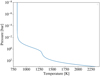 |
Fig. 1 Temperature–pressure profile used in our fiducial model, generated using Eq. (2), using the parameters listed in Table 2. |
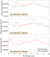 |
Fig. 2 Calculated transmission spectra of a VULCAN model with all stellar flux removed <200 nm (top), <300 nm (middle), and <350 nm (bottom). Removing the flux below 200 nm and 300 nm still produces a SO2 signal, whereas removing the flux below 350 nm prevents the production of SO2. |
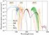 |
Fig. 3 Photodissociation cross section of H2O, SH, S2, and SO2 as a function of wavelength. The data are from the VULCAN photochemical kinetics code, which obtains cross sections from the Leiden Observatory database (Heays et al. 2017). |
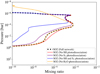 |
Fig. 4 Mixing ratio of SO2 in VULCAN models with various photodissociation reactions switched off to isolate their contribution. If H2O photodissociation is turned off, SO2 is less abundant at 10−6 bar. If both S2 and SH photodissociation are turned off, SO2 is less abundant at 10−4 bar. If only S2 or SH photodissociation is turned off, the SO2 abundance is not affected significantly. |
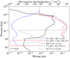 |
Fig. 5 Mixing ratio of SO2 (solid line) and net reaction rates of various chemical reactions, subtracting the reverse reaction rate from the forward reaction rate (dash-dotted lines) in the fiducial model. We see that reactions (10), (11), (12), and (13) are particularly pronounced in the region of the atmosphere where SO2 is abundant. |
4.2 Rate analysis
In this section, we turn to an analysis of the reaction rates of the chemical reactions discussed in the previous section to investigate which specific reactions are active in the various scenarios discussed above. In Fig. 5 we plot the reaction rates of reactions (6), (10), (11), (12), and (13) in our fiducial model. We see that these reactions are active at similar rates in the layers where SO2 is abundant, providing a further indication of their involvement in the pathway to SO2. Further analysis shows that the model reaches near-chemical equilibrium in the deeper parts of the atmosphere (see Fig. A.1).
From Fig. 4 it becomes clear that at around 10−6 bar the mixing ratio of SO2 is unaltered by the absence of SH and S2 photodissociation. This raises the question what the source of atomic sulfur is at this layer without these reactions. In Fig. 6, we see that the hydrogen abstraction of SH takes over as the source of atomic S at 10−6 bar. The photodissociation of H2O at these layers provides sufficient amounts of atomic H to drive this reaction forward. In deeper layers of the atmosphere H2O photodissociation does not take place, and there is insufficient production of atomic H for the hydrogen abstraction of SH to occur, preventing the formation of atomic S.
In addition, Fig. 4 shows that turning off H2O photodissociation reduces the mixing ratio of SO2 around 10−6 bar, but not at higher pressures of around 10−4 bar. In Section 4.1, we claim it was the hydrogen abstraction of H2, driven by the photodissociation of SH, that drove the production of atomic H, which subsequently led to the hydrogen abstraction of H2O.
We investigate this in Fig. 7, where we plot the reaction rates of the photodissociation and hydrogen abstraction of H2O. At lower pressures, OH is provided by photodissociation of H2O, but at higher pressures, it is provided by the hydrogen abstraction of H2O. This confirms our claim that there are two separate pathways to SO2, depending on the layer of the atmosphere.
This leaves us with an unresolved problem: the mechanism responsible for producing SO2 in our model with no flux below 300 nm. In Fig. 3, we plot the photodissociation cross section of SH and S2 as a function of wavelength. We see that there is still significant absorption in the range 300–350 nm, which is in line with our result that stellar flux in this wavelength range is sufficient to lead to the production of SO2. Figure 8 shows the reaction rate of H2O hydrogen abstraction, which shows that without flux at wavelengths shorter than 300 nm this reaction shifts completely to the right. This suggests that in a model atmosphere without flux at wavelengths shorter than 300 nm, hydrogen abstraction of H2O completely takes over as the source of OH in the pathway to SO2.
The overarching scenario that arises is that the SH-H2S feedback loop is the main provider of atomic S for the production of SO2. H2O photodissociation is the main provider of OH at pressures of around 10−6 bar, whereas H2O hydrogen abstraction is responsible for providing OH at higher pressures of approximately 10−4 bar.
In a final experiment on the stellar flux, we ran models with all flux removed above 200 and 300 nm to quantify the impact of these parts of the SED on the transit spectrum. We show these results in Fig. 9. Here we see that flux between 200 and 300 nm contributes significantly to the visibility of SO2 in the transit spectrum, whereas flux at wavelengths above 300 nm does not. However, we saw in Fig. 2 that flux between 300 and 350 nm produces a significant amount of SO2 in the absence of flux below 300 nm. We conclude that flux between 300 and 350 nm only contributes significantly to the formation of SO2 when no flux at lower wavelengths is present that photodissociates SO2. This situation occurs in deeper parts of the atmosphere, which are shielded from XUV and UV radiation that dissociates SO2, while it is still subjected to near-ultraviolet (NUV) radiation above 300 nm that leads to the production of SO2. This effect is responsible for the dependence of SO2 formation on surface gravity, which we show in Sect. 4.3.
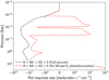 |
Fig. 6 Net reaction rate of SH hydrogen abstraction, subtracting the reverse reaction rate from the forward reaction rate. This figure shows that in the absence of SH and S2 photodissociation, at 10−6 bar the hydrogen abstraction of SH is able to take over as the source of atomic S in the pathway to SO2. |
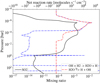 |
Fig. 7 Mixing ratio of SO2 (solid line) and net reaction rates of H2O hydrogen abstraction and photodissociation, subtracting the reverse reaction rate from the forward reaction rate (dash-dotted lines) in the fiducial model. At 10−6 bar, OH is supplied by H2O photodissociation. At 10−4 bar, OH is supplied by H2O hydrogen abstraction. |
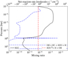 |
Fig. 8 Mixing ratio of SO2 (solid line) and net reaction rates of H2O hydrogen abstraction and photodissociation, subtracting the reverse reaction rate from the forward reaction rate (dash-dotted lines) in the model with no flux <300 nm. We see that in a model without stellar flux <300 nm, no H2O photodissociation occurs, and that OH is produced by H2O hydrogen abstraction in almost all layers of the atmosphere. |
4.3 The influence of surface gravity
Inspired by the recent detection of SO2 in the atmosphere of WASP-107b (Dyrek et al. 2024), a planet with an extraordinarily low surface gravity of 309 cm/s2, we investigated the influence of the surface gravity on the mixing ratios and visibility of SO2. To do this, first we changed the TP profile of our fiducial model to an isothermal TP profile. The reason we chose to do this was to allow us to isolate the effect of surface gravity. The parameterized TP profile we used, as described in Section 2, is a parameterization that depends on the surface gravity, meaning that if we change the surface gravity we also change the TP profile. Replacing the TP profile with an isothermal profile does not significantly impact the mixing ratios of SO2, likely due to the fact that our parameterized TP profile is also isothermal below a pressure of 10−2 bar. We set the isothermal temperature of our atmosphere at T = 740 K, the effective temperature of WASP-107b (Dyrek et al. 2024).
In Fig. 10, we plot the transmission spectra of our isothermal model for three values of the surface gravity. We see in this plot that the visibility of SO2 in the transmission spectrum increases as the surface gravity decreases. In computing the spectrum, the pressure coordinates are translated to geometric coordinates under the assumption of hydrostatic equilibrium. A lower surface gravity translates to an extended scale height, and therefore increased transit depth, which causes part of the increase in visibility of SO2. Therefore, to isolate the effect of the increased mixing ratios on the visibility of SO2 in the spectrum, in Fig. 11, we take the mixing ratios of these atmospheres, but keep the surface gravity at 2250 cm/s2 when computing the transmission spectrum. This produces a similar result, although the effect is less pronounced, from which we conclude that the effect on the transmission spectrum is due to the larger scale height and to the increase in SO2 mixing ratio brought about by lower surface gravity.
In Fig. 12, we plot the mixing ratios of SO2 in these three models, as well as the rate of SO2 photodissociation. We see that the mixing ratio of SO2 increases and that the photodissociation rate of SO2 decreases as the surface gravity is decreased. We interpret this as the stellar UV radiation reaching higher pressure parts of the atmosphere in a model with higher surface gravity, which can be expected from the relation between optical depth, pressure, and surface gravity (assuming constant gravity and hydrostatic equilibrium):
 (19)
(19)
Here P is the pressure, τ is the optical depth, g is the surface gravity, and κth is the opacity to infrared radiation. At lower surface gravity, the point where τ = 1 is reached for radiation at a particular wavelength is at a lower pressure. We conclude that a lower surface gravity prevents SO2 photodissociation from reaching the deeper layers of the atmosphere. The NUV flux that produces SO2 at these layers is also absorbed in higher layers, so the natural question that arises is why this nonetheless leads to an increase in the mixing ratios.
In Fig. 2, we show that in a situation with only stellar flux above 300 nm there is a strong production of SO2. However, Fig. 9 shows that removing the flux above 300 nm does not impact the production of SO2. We concluded that stellar flux between 300 and 350 nm only produces SO2 in the absence of stellar flux at shorter wavelengths that dissociates SO2.
A situation similar to this arises deep in an atmosphere with a low surface gravity. To show this, in Fig. 13 we plot the actinic flux (the radiation intensity integrated over all directions) in an atmosphere with high and low surface gravity. In both situations, stellar flux between 300 and 350 nm reaches deep into the atmosphere. At pressures higher than 10−4 bar, this does not lead to the production of significant amounts of SO2 because high pressures strongly drive the abundances toward chemical equilibrium. Low surface gravity prevents stellar flux shorter than 200 nm from reaching the layers around 10−4 bar. The photodissociation cross section of SO2 decreases as a function of wavelength (see Fig. 3), so while the flux in the 300-350 nm window is still able to reach the layers around 10−4 bar when the surface gravity is low, which leads to the production of SO2, the photodissociation of SO2 is strongly diminished. This leads to an increase in the mixing ratio of SO2, which in turn leads to an increased visibility in the transit spectrum. We note that the SO2 peak shifts upward slightly, so the presence of flux between 300 and 350 nm is not completely able to compensate for the upward shift of the NUV absorption in the atmosphere.
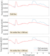 |
Fig. 9 Transit spectrum of our fiducial model (top panel), and the same model but with all flux removed above 300 nm (middle panel) and all flux removed above 200 nm (bottom panel). This figure shows the contribution of the flux between 200 and 300 nm and the contribution of flux >300 nm to the transit spectrum. |
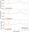 |
Fig. 10 Visibility of SO2 in the transmission spectrum as a function of surface gravity in the model with an isothermal TP profile of 740 K. We see that a lower surface gravity leads to a greater visibility of SO2 in the transmission spectrum. |
 |
Fig. 11 Same as in Fig. 10, but with the surface gravity set to 2250 cm/s2 for all models when computing the spectrum, so that the change in the spectrum is attributable only to the change in mixing ratios. |
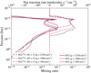 |
Fig. 12 Mixing ratios of SO2 (solid lines) and the rate of the dominant SO2 photodissociation branch (dash-dotted lines) in the fiducial model with an isothermal TP profile of 740 K. We see that the mixing ratio of SO2 is elevated and photodissociation of SO2 is diminished in the models with lower surface gravity. |
4.4 The influence of temperature
Reaction rates in an atmosphere are strongly dependent on the temperature of the atmosphere, and uncertainties still exist in the TP structure of exoplanetary atmospheres. For these two reasons, we investigated the effect of changing the temperature of our model atmosphere on the chemical pathway to SO2. We changed the temperature by shifting it throughout the vertical column by a set amount.
We investigated the effect of changing the temperature of our atmosphere by 100 K and 50 K. The only significant difference we find is the direction of the reaction SH + H → S + H2 in the upper layer of the atmosphere. We show this effect in Fig. 14. Here we see that this reaction runs to the right at 10−6 bar if we lower the temperature of the atmosphere, whereas if we increase the temperature, it runs to the left.
This suggests a temperature dependence of the pathway to SO2 in the upper layer of the atmosphere. At lower temperatures (below ~800 K) around 10−6 bar, the pathway to SO2 occurs as described by Tsai et al. (2023a). Around 10−4 bar, photodis-sociation of SH and S2 is still the pathway to SO2, even at lower temperatures. At higher temperatures, the reaction SH + H → S + H2 runs to the left, and the photochemical dissociation of SH and S2 drives the liberation of sulfur from H2S at all layers.
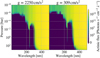 |
Fig. 13 Actinic flux in the atmosphere for two values of the surface gravity. The stellar flux is absorbed in the higher layers of the atmosphere for a lower surface gravity. |
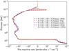 |
Fig. 14 Net reaction rate of SH hydrogen abstraction, subtracting the reverse from the forward rate. We show the output of five VULCAN models, one with the fiducial TP profile as described in Fig. 1, the others with the temperature profile shifted by a set amount throughout the atmospheric column. We see that if we decrease the temperature, at a pressure of 10−6 bar, SH reacts with atomic H to produce atomic sulfur. |
5 Discussion
We have shown that stellar flux between 300 and 350 nm is a sufficient condition for the formation of SO2. Furthermore, the photodissociation of SH and S2 plays a significant role in the formation of SO2 in deeper layers of the atmosphere. Hydrogen abstraction of H2O is the predominant source of OH in these deeper layers, and photodissociation of H2O is the source of OH in higher layers. In this section, we look at the implications for recent and potentially forthcoming SO2 observations.
5.1 The importance of stellar flux
Currently, the UV flux of the host star is one of the major uncertainties in photochemical modeling. Most research to date has taken an approach that combines observations and theoretical models to reconstruct the stellar UV field. Based on the conclusions from Tsai et al. (2023a), it was logical to assume that stellar UV flux below 200 nm is a necessary condition to observe SO2, but this paper suggests that we can relax this assumption. Quiescent stars with low UV fluxes are an equally promising target when it comes to the detection of photochemistry.
One may argue that the situation of all flux removed below a certain wavelength is an unphysical situation, but the question is whether this is in fact true. In current photochemical models, the upper boundary is where the atmosphere ends, and it is assumed that there is no UV absorption above the upper boundary. However, models and observations of atmospheric escape suggest that strong XUV absorption in the exosphere is necessary to drive the hydrodynamic escape of the atmosphere (Oklopčić & Hirata 2018; Spake et al. 2018; Allart et al. 2018; MacLeod & Oklopčić 2022; Linssen & Oklopčić 2023; Nail et al. 2024; Zhang et al. 2023; Owen & Schlichting 2024). Most of the absorption will be due to atomic hydrogen, and therefore occurs below the Lyman-α line, suggesting that this effect is limited to the upper atmosphere. To our knowledge, photochemical models that filter the input stellar spectrum through the exosphere have not yet been considered, and we suggest it as a direction for future research.
The opposite situation can also occur, where there is significant stellar flux in the UV, but lower flux in the NUV. This is the situation in M stars that have significant chromospheric activity, but due to their low effective temperatures have low photospheric flux at higher wavelengths. We suggest targeting close-in gas giants around these stars to investigate the presence of SO2. We expect SO2 to be produced only in higher layers of the atmosphere in these planets, which should lead to a lower visibility of SO2 in the spectrum.
5.2 Temperature-dependent UV cross sections
Laboratory measurements of the UV cross sections of molecules are usually obtained at room temperature, and there is a need for the expansion of these measurements to higher temperature ranges, such as those found in hot gas giants (Fortney et al. 2019; Venot et al. 2018). We used room temperature cross sections for the modeling performed for this paper. It was suggested by Heays et al. (2017) that a temperature increase of only a few hundred kelvins should not impact the UV cross sections much for many molecules. For those molecules with transitions between excited vibrational states, however, the impact on the cross sections can in fact be significant. Temperature-dependent cross sections for SH are available from the ExoMol project (Gorman et al. 2019), who found that the UV cross section increases significantly as the temperature is increased. This occurs in the important 200–350 nm window, and above 350 nm. This potentially leads to increased SH photodissociation, and thus to an increased rate of photochemically induced H2S destruction, which further underscores the importance of the results of this paper for the production of SO2. These cross sections have been implemented in VULCAN, and a number of preliminary tests can be found in Tsai et al. (2021). In addition, temperature dependent cross sections are also available for SO2, although they have only been taken for one temperature to date (Fateev 2021). We leave an investigation of the effect of temperature dependent UV cross sections to a future study.
5.3 The case of WASP-107b
At the time of writing this paper, SO2 has been detected in the atmospheres of WASP-39b (Rustamkulov et al. 2023) and WASP-107b (Dyrek et al. 2024). In light of the results of this paper, the WASP-107b detection is particularly interesting, where alongside SO2 silicate clouds were also detected.
The pressure level at which the clouds were detected was still relatively poorly constrained. Using two different retrieval codes, the pressure level of the clouds was found to be either 10−5 bar or 10−3 bar. Additionally, no constraints were placed on the longitude of the clouds, due to the 1D nature of the retrieval framework. Silicate clouds are significant absorbers of UV radiation, so the precise location of the clouds matters significantly for the photochemistry that can occur in an exoplanet. Unfortunately, full cloud coverage obscures the visibility of chemical species below the clouds. However, in the case of WASP-107b the cloud coverage was relatively thin, and the atmospheric layers below the clouds contributed partially to the transit spectrum, although this was not the case for the SO2 absorption, which originated from above the clouds.
In this paper, we found that NUV radiation leads to detectable quantities of photochemically produced SO2 at pressures as high as 10−4 bar in a cloud-free model. On a planet with a sufficiently low atmospheric temperature, such as WASP-107b, silicate cloud formation can take place on the dayside of the planet, which would be able to partially insulate deeper layers of the atmosphere from the effects of photochemistry. Further complexity is brought about by the effect of global chemical transport around the equator, which can transport the products of photochemistry from the dayside to the nightside, as has been investigated by Baeyens, Robin et al. (2024) and Tsai et al. (2023b), among others. It is still an open question to what extent partial cloud coverage affects the formation of SO2 below the clouds. We suggest an investigation of the competing effects of clouds and photochemistry as the direction of a potential future study with the available 2D photochemical kinetics codes, for example (Tsai et al. 2024). Planets with thin cloud coverage such as WASP-107b may present an opportunity to constrain the efficiency of photochemistry below the cloud layer.
6 Summary and conclusion
We studied the chemical pathways leading to SO2, as well as the dependence on the stellar flux field. We arrived at the following conclusions:
Stellar flux between 300 and 350 nm leads to a strong production of SO2 in the absence of stellar flux below 300 nm.
Near-UV driven photochemical dissociation of SH and S2 leads to the production of atomic S and H, which subsequently leads to the formation of SO2;
The pathway to SO2 is dependent on the atmospheric layer where it is formed. At pressures around 10−4 bar, it depends on the hydrogen abstraction of H2O. At pressures around 10−6 bar, it depends on the photochemical dissociation of H2O;
A lower surface gravity elevates the mixing ratio of SO2 and therefore increases its visibility in the transmission spectrum. This is due to the increased scale height of the atmosphere and stellar radiation being absorbed higher up in the atmosphere;
Hydrogen abstraction of SH plays a role in the pathway to SO2 at pressures around 10−6 bar at temperatures below 800 K.
Acknowledgements
S.-M.T. acknowledges support from NASA Exobiology Grant No. 80NSSC20K1437 and the University of California at Riverside. L.D. acknowledges funding from the KU Leuven Interdisciplinary Grant (IDN/19/028), the European Union H2020-MSCA-ITN-2019 under Grant no. 860470 (CHAMELEON) and the FWO research grant G086217N.
Appendix A Test of chemical equilibrium
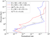 |
Fig. A.1 Normalized reaction rates (abs(forward reaction rate - reverse reaction rate)/(forward reaction rate)) of various chemical reactions in the fiducial model. Normalized reaction rates become comparatively small in the bottom regions of the atmosphere, indicating these regions approach chemical equilibrium. |
References
- Allart, R., Bourrier, V., Lovis, C., et al. 2018, Science, 362, 1384 [Google Scholar]
- Asplund, M., Grevesse, N., Sauval, A. J., & Scott, P. 2009, ARA&A, 47, 481 [NASA ADS] [CrossRef] [Google Scholar]
- Baeyens, R., Désert, J.-M., Petrignani, A., Carone, L., & Schneider, A. D. 2024, A&A, 686, A24 [NASA ADS] [CrossRef] [EDP Sciences] [Google Scholar]
- Boley, A. C. 2009, ApJ, 695, L53 [NASA ADS] [CrossRef] [Google Scholar]
- Chubb, K. L., Rocchetto, M., Yurchenko, S. N., et al. 2021, A&A, 646, A21 [NASA ADS] [CrossRef] [EDP Sciences] [Google Scholar]
- Chubb, K. L., Robert, S., Sousa-Silva, C., et al. 2024, arXiv e-prints [arXiv: 2404.02188] [Google Scholar]
- Dyrek, A., Min, M., Decin, L., et al. 2024, Nature, 625, 51 [Google Scholar]
- Fateev, A. 2021, JQSRT, https://exomol.com/data/data-types/photo/SO2/32S-16O2/DTU/#32S-16O2-DTU-photo [Google Scholar]
- Fortney, J., Robinson, T. D., Domagal-Goldman, S., et al. 2019, Astro2020: Decadal Survey on Astronomy and Astrophysics, 2020, 146 [Google Scholar]
- Goody, R., West, R., Chen, L., & Crisp, D. 1989, J. Quant. Spec. Radiat. Transf., 43, 191 [NASA ADS] [Google Scholar]
- Gordon, I. E., Rothman, L. S., Hill, C., et al. 2017, J. Quant. Spec. Radiat. Transf., 203, 3 [NASA ADS] [CrossRef] [Google Scholar]
- Gorman, M. N., Yurchenko, S. N., & Tennyson, J. 2019, MNRAS, 490, 1652 [Google Scholar]
- Guillot, T. 2010, A&A, 520, A27 [NASA ADS] [CrossRef] [EDP Sciences] [Google Scholar]
- Heays, A. N., Bosman, A. D., & van Dishoeck, E. F. 2017, A&A, 602, A105 [NASA ADS] [CrossRef] [EDP Sciences] [Google Scholar]
- Hobbs, R., Rimmer, P. B., Shorttle, O., & Madhusudhan, N. 2021, MNRAS, 506, 3186 [NASA ADS] [CrossRef] [Google Scholar]
- Lacis, A. A., & Oinas, V. 1991, J. Geophys. Res., 96, 9027 [Google Scholar]
- Linssen, D. C., & Oklopcic, A. 2023, A&A, 675, A193 [NASA ADS] [CrossRef] [EDP Sciences] [Google Scholar]
- MacLeod, M., & Oklopcic, A. 2022, ApJ, 926, 226 [NASA ADS] [CrossRef] [Google Scholar]
- Madhusudhan, N. 2019, ARA&A, 57, 617 [NASA ADS] [CrossRef] [Google Scholar]
- Min, M., Ormel, C. W., Chubb, K., Helling, C., & Kawashima, Y. 2020, A&A, 642, A28 [NASA ADS] [CrossRef] [EDP Sciences] [Google Scholar]
- Moses, J. I., Visscher, C., Fortney, J. J., et al. 2011, ApJ, 737, 15 [Google Scholar]
- Nail, F., Oklopcic, A., & MacLeod, M. 2024, A&A, 684, A20 [NASA ADS] [CrossRef] [EDP Sciences] [Google Scholar]
- Öberg, K. I., Murray-Clay, R., & Bergin, E. A. 2011, ApJ, 743, L16 [Google Scholar]
- Oklopčić, A., & Hirata, C. M. 2018, ApJ, 855, L11 [Google Scholar]
- Ormel, C. W., & Min, M. 2019, A&A, 622, A121 [NASA ADS] [CrossRef] [EDP Sciences] [Google Scholar]
- Owen, J. E., & Schlichting, H. E. 2024, MNRAS, 528, 1615 [NASA ADS] [CrossRef] [Google Scholar]
- Polman, J., Waters, L. B. F. M., Min, M., Miguel, Y., & Khorshid, N. 2023, A&A, 670, A161 [NASA ADS] [CrossRef] [EDP Sciences] [Google Scholar]
- Rafikov, R. R. 2005, ApJ, 621, L69 [Google Scholar]
- Rimmer, P. B., Jordan, S., Constantinou, T., et al. 2021, PSJ, 2, 133 [NASA ADS] [Google Scholar]
- Rothman, L. S., Gordon, I. E., Barber, R. J., et al. 2010, J. Quant. Spec. Radiat. Transf., 111, 2139 [NASA ADS] [CrossRef] [Google Scholar]
- Rustamkulov, Z., Sing, D. K., Mukherjee, S., et al. 2023, Nature, 614, 659 [NASA ADS] [CrossRef] [Google Scholar]
- Southworth, J. 2010, MNRAS, 408, 1689 [Google Scholar]
- Spake, J. J., Sing, D. K., Evans, T. M., et al. 2018, Nature, 557, 68 [Google Scholar]
- Tennyson, J., Yurchenko, S. N., Al-Refaie, A. F., et al. 2016, J. Mol. Spectrosc., 327, 73 [Google Scholar]
- Tsai, S.-M., Lyons, J. R., Grosheintz, L., et al. 2017, ApJS, 228, 20 [NASA ADS] [CrossRef] [Google Scholar]
- Tsai, S.-M., Malik, M., Kitzmann, D., et al. 2021, ApJ, 923, 264 [NASA ADS] [CrossRef] [Google Scholar]
- Tsai, S.-M., Lee, E. K. H., Powell, D., et al. 2023a, Nature, 617, 483 [CrossRef] [Google Scholar]
- Tsai, S.-M., Moses, J. I., Powell, D., & Lee, E. K. H. 2023b, ApJ, 959, L30 [NASA ADS] [CrossRef] [Google Scholar]
- Tsai, S.-M., Parmentier, V., Mendonça, J. M., et al. 2024, ApJ, 963, 41 [NASA ADS] [CrossRef] [Google Scholar]
- Turrini, D., Schisano, E., Fonte, S., et al. 2021, ApJ, 909, 40 [Google Scholar]
- Venot, O., Hébrard, E., Agúndez, M., et al. 2012, A&A, 546, A43 [NASA ADS] [CrossRef] [EDP Sciences] [Google Scholar]
- Venot, O., Bénilan, Y., Fray, N., et al. 2018, A&A, 609, A34 [NASA ADS] [CrossRef] [EDP Sciences] [Google Scholar]
- Yurchenko, S. N., Al-Refaie, A. F., & Tennyson, J. 2018, A&A, 614, A131 [NASA ADS] [CrossRef] [EDP Sciences] [Google Scholar]
- Zahnle, K., Marley, M. S., Freedman, R. S., Lodders, K., & Fortney, J. J. 2009, ApJ, 701, L20 [Google Scholar]
- Zhang, Z., Morley, C. V., Gully-Santiago, M., et al. 2023, Sci. Adv., 9, eadf8736 [Google Scholar]
All Tables
All Figures
|
Fig. 1 Temperature–pressure profile used in our fiducial model, generated using Eq. (2), using the parameters listed in Table 2. |
| In the text | |
|
Fig. 2 Calculated transmission spectra of a VULCAN model with all stellar flux removed <200 nm (top), <300 nm (middle), and <350 nm (bottom). Removing the flux below 200 nm and 300 nm still produces a SO2 signal, whereas removing the flux below 350 nm prevents the production of SO2. |
| In the text | |
|
Fig. 3 Photodissociation cross section of H2O, SH, S2, and SO2 as a function of wavelength. The data are from the VULCAN photochemical kinetics code, which obtains cross sections from the Leiden Observatory database (Heays et al. 2017). |
| In the text | |
|
Fig. 4 Mixing ratio of SO2 in VULCAN models with various photodissociation reactions switched off to isolate their contribution. If H2O photodissociation is turned off, SO2 is less abundant at 10−6 bar. If both S2 and SH photodissociation are turned off, SO2 is less abundant at 10−4 bar. If only S2 or SH photodissociation is turned off, the SO2 abundance is not affected significantly. |
| In the text | |
|
Fig. 5 Mixing ratio of SO2 (solid line) and net reaction rates of various chemical reactions, subtracting the reverse reaction rate from the forward reaction rate (dash-dotted lines) in the fiducial model. We see that reactions (10), (11), (12), and (13) are particularly pronounced in the region of the atmosphere where SO2 is abundant. |
| In the text | |
|
Fig. 6 Net reaction rate of SH hydrogen abstraction, subtracting the reverse reaction rate from the forward reaction rate. This figure shows that in the absence of SH and S2 photodissociation, at 10−6 bar the hydrogen abstraction of SH is able to take over as the source of atomic S in the pathway to SO2. |
| In the text | |
|
Fig. 7 Mixing ratio of SO2 (solid line) and net reaction rates of H2O hydrogen abstraction and photodissociation, subtracting the reverse reaction rate from the forward reaction rate (dash-dotted lines) in the fiducial model. At 10−6 bar, OH is supplied by H2O photodissociation. At 10−4 bar, OH is supplied by H2O hydrogen abstraction. |
| In the text | |
|
Fig. 8 Mixing ratio of SO2 (solid line) and net reaction rates of H2O hydrogen abstraction and photodissociation, subtracting the reverse reaction rate from the forward reaction rate (dash-dotted lines) in the model with no flux <300 nm. We see that in a model without stellar flux <300 nm, no H2O photodissociation occurs, and that OH is produced by H2O hydrogen abstraction in almost all layers of the atmosphere. |
| In the text | |
|
Fig. 9 Transit spectrum of our fiducial model (top panel), and the same model but with all flux removed above 300 nm (middle panel) and all flux removed above 200 nm (bottom panel). This figure shows the contribution of the flux between 200 and 300 nm and the contribution of flux >300 nm to the transit spectrum. |
| In the text | |
|
Fig. 10 Visibility of SO2 in the transmission spectrum as a function of surface gravity in the model with an isothermal TP profile of 740 K. We see that a lower surface gravity leads to a greater visibility of SO2 in the transmission spectrum. |
| In the text | |
|
Fig. 11 Same as in Fig. 10, but with the surface gravity set to 2250 cm/s2 for all models when computing the spectrum, so that the change in the spectrum is attributable only to the change in mixing ratios. |
| In the text | |
|
Fig. 12 Mixing ratios of SO2 (solid lines) and the rate of the dominant SO2 photodissociation branch (dash-dotted lines) in the fiducial model with an isothermal TP profile of 740 K. We see that the mixing ratio of SO2 is elevated and photodissociation of SO2 is diminished in the models with lower surface gravity. |
| In the text | |
|
Fig. 13 Actinic flux in the atmosphere for two values of the surface gravity. The stellar flux is absorbed in the higher layers of the atmosphere for a lower surface gravity. |
| In the text | |
|
Fig. 14 Net reaction rate of SH hydrogen abstraction, subtracting the reverse from the forward rate. We show the output of five VULCAN models, one with the fiducial TP profile as described in Fig. 1, the others with the temperature profile shifted by a set amount throughout the atmospheric column. We see that if we decrease the temperature, at a pressure of 10−6 bar, SH reacts with atomic H to produce atomic sulfur. |
| In the text | |
|
Fig. A.1 Normalized reaction rates (abs(forward reaction rate - reverse reaction rate)/(forward reaction rate)) of various chemical reactions in the fiducial model. Normalized reaction rates become comparatively small in the bottom regions of the atmosphere, indicating these regions approach chemical equilibrium. |
| In the text | |
Current usage metrics show cumulative count of Article Views (full-text article views including HTML views, PDF and ePub downloads, according to the available data) and Abstracts Views on Vision4Press platform.
Data correspond to usage on the plateform after 2015. The current usage metrics is available 48-96 hours after online publication and is updated daily on week days.
Initial download of the metrics may take a while.