| Issue |
A&A
Volume 670, February 2023
|
|
|---|---|---|
| Article Number | A161 | |
| Number of page(s) | 11 | |
| Section | Planets and planetary systems | |
| DOI | https://doi.org/10.1051/0004-6361/202244647 | |
| Published online | 22 February 2023 | |
H2S and SO2 detectability in hot Jupiters
Sulphur species as indicators of metallicity and C/O ratio
1
Department of Astrophysics/IMAPP, Radboud University Nijmegen,
PO Box 9010,
6500 GL
Nijmegen, The Netherlands
2
SRON Netherlands Institute for Space Research,
Niels Bohrweg 4,
2333 CA
Leiden, The Netherlands
e-mail: This email address is being protected from spambots. You need JavaScript enabled to view it.
3
Sterrewacht leiden, University of Leiden,
Niels Bohrweg 2,
2333 CA
Leiden, The Netherlands
4
Anton Pannekoek Institute for Astronomy, University of Amsterdam,
Science Park 904,
1098 XH
Amsterdam, The Netherlands
Received:
31
July
2022
Accepted:
14
November
2022
Abstract
Context. The high cosmic abundance, the intermediate volatility, and the chemical properties of sulphur allow sulphur-bearing species to be used as tracers of the chemical processes in the atmospheres of hot Jupiter exoplanets. Nevertheless, despite their properties and relevance as tracers of the giant planets’ formation histories, little attention has been paid to these species in the context of hot Jupiter atmospheres.
Aims. In this paper, we provide an overview of the abundances of sulphur-bearing species in hot Jupiter atmospheres under different conditions and explore their observability.
Methods. We used the photochemical kinetics code VULCAN to model hot Jupiter atmospheric disequilibrium chemistry. Transmission spectra for these atmospheres were created using the modelling framework ARCiS. We varied model parameters such as the diffusion coefficient Kzz, and we studied the importance of photochemistry on the resulting mixing ratios. Furthermore, we varied the chemical composition of the atmosphere by increasing the metallicity from solar to ten times solar. We also explored different C/O ratios.
Results. We find that H2S and SO2 are the best candidates for detection between 1 and 10 μm, using a spectral resolution that is representative of the instruments on board the James Webb Space Telescope (JWST). H2S is easiest to detect at an equilibrium temperature of ~1500 K, and with C/O ratios between 0.7 and 0.9, with the ideal value increasing slightly for increasing metallicity. SO2 is most likely to be detected at an equilibrium temperature of ~1000 K at low C/O ratios and high metallicities. Nevertheless, among these two molecules, we expect SO2 detection to be more common, as it is detectable in scenarios more favoured by formation models.
Conclusions. We conclude that H2S and SO2 will most likely be detected in the coming years with the JWST, and that the detection of these species will provide information on atmospheric processes and planet formation scenarios.
Key words: planets and satellites: atmospheres / planets and satellites: gaseous planets / infrared: planetary systems
© The Authors 2023
 Open Access article, published by EDP Sciences, under the terms of the Creative Commons Attribution License (https://creativecommons.org/licenses/by/4.0), which permits unrestricted use, distribution, and reproduction in any medium, provided the original work is properly cited.
This article is published in open access under the Subscribe to Open model. This email address is being protected from spambots. You need JavaScript enabled to view it. to support open access publication.
1 Introduction
Observations with Hubble, Spitzer, and ground-based telescopes have revealed a wide variety of atmospheric properties (Madhusudhan 2019) and the more observations we have, the stronger the diversity observed in exoplanet atmospheres. The challenge is to understand this wide diversity, and place it in the context of planet formation scenarios (Khorshid et al. 2022; Turrini et al. 2021). In particular, abundant species such as C-, N-, O- and S-bearing species can elucidate both the processes that occur in the atmosphere and at the same time provide clues on the formation history of the planet.
Sulphur is an important chemical element in this context. This is because of its cosmic abundance, its ability to bind to carbon and oxygen, its role in atmospheric chemistry, and its intermediate volatility when compared to highly refractory rock-forming elements such as Fe, Mg, and Si, and volatile species such as C and N. Recent planet formation models have suggested that the combined use of the highly volatile N and the much more refractory S abundances in planetary atmospheres may be important to break degeneracies in planet formation scenarios when using only C and O (Turrini et al. 2021). Moreover, sulphur may be refractory and could be used as a proxy for metallicity (Kama et al. 2019; Turrini et al. 2021).
Atmospheric models of exoplanets have mainly focused on hydrogen, carbon, oxygen, and nitrogen because they are the most abundant elements in the Sun when excluding the non-reactive noble gases. This is due to the complexity of these models and the difficulty of obtaining accurate reaction rates. Nevertheless, efforts have been made to study sulphur chemistry (Zahnle et al. 2009; Wang et al. 2017), and sulphur networks are included in codes such as LEVI (Hobbs et al. 2021) and VULCAN (Tsai et al. 2017; Tsai et al. 2021). Both models find that sulphur can play a significant role in the overall atmospheric chemistry by offering a faster pathway for liberating oxygen from H2O.
Motivated by these efforts, in this paper we study the main sulphur-bearing species in hot Jupiter atmospheres and their potential detectability. We explore different potential scenarios such as different metallicities and C/O ratios, exploring the best conditions to detect these molecules and helping in the interpretation of future James Webb Space Telescope (JWST) data. A better quantitative understanding of the main sulphur reservoirs in molecular clouds and planet-forming disks is being built up from ALMA and other millimetre wave telescopes (Laas & Caselli 2019; Cazaux et al. 2022; Le Gal et al. 2021; Codella et al. 2021; Cernicharo et al. 2021), which will, in the future, allow us to put the sulphur abundance in exoplanetary atmospheres into context.
This paper is organised as follows. In Sect. 2 we describe the method we used to calculate the chemical composition of hot Jupiter atmospheres in the form of mixing ratios as a function of pressure, and the forward model we used to generate transmission spectra in the wavelength range of interest for observations with the JWST. Section 3 describes the resulting atmospheric mixing ratios, and the emerging transmission spectra. We also varied some important parameters that affect the mixing ratios of molecular species of interest. In Sect. 4 we focus on H2S and SO2, the two most promising sulphur-bearing molecules with respect to their detectability. In Sect. 5 we discuss our results, and Sect. 6 contains the conclusions of this study.
Standard parameters used within VULCAN.
2 Method
2.1 Disequilibrium chemistry calculations
We used the open-source photochemical kinetics code VULCAN (Tsai et al. 2017; Tsai et al. 2021) to model hot Jupiter atmospheres. Within VULCAN we used a C-H-N-O-S chemical network, expanded from the C-H-N-O network of Tsai et al. (2017). The network consists of 87 species, approximately 500 forward chemical reactions, the associated reverse reactions, and 60 photodissociation branches. The included sulphur species are S, S2, S3, S4, S8, SH, HSO, H2S, SO, CS, COS, CS2, NS, HS2, SO2, HCS, S2O, CH3SH, and CH3S. For the planetary parameters, we used standard values for HD 189733 b as shown in Table 1. The stellar flux of HD 189733 was taken from Moses et al. (2011). We used protosolar elemental abundances from Lodders et al. (2009), hereafter referred to as solar abundances. For the diffusion coefficient, we assumed a constant value of 109 cm2/s. The effect of this choice and the overall dependence of the results on the value of the diffusion coefficient are discussed in Sect. 5.
We used 150 vertical atmospheric layers, resulting in roughly six layers per pressure scale height, as recommended for VULCAN, to ensure visibly smooth profiles. For each layer the number densities of each species were computed based on the number densities at the preceding timestep, the reaction rates of each reaction, the stellar flux reaching the layer for photodissociation, and the diffusion coefficient for mixing between each layer. For the convergence parameters, we used the recommended values δ=0.01 and ϵ=10−4 s−1 associated with the conditions  and
and  , where
  and
and  ‚ with i denoting the species, j the layer, and k the timestep. The convergence criteria ensured consistent results and were the same as those recommended by Tsai et al. (2017). We found that the relative tolerance for adjusting the step size had to be changed often to ensure convergence without large elemental losses. Simulations were redone with different values for this tolerance if elemental losses or gains of more than one percent occurred. A summary, alongside other parameters used in VULCAN, is shown in Table 1.
We mainly focus on two different temperature-pressure (TP) profiles, a TP-profile from Moses et al. (2011) for HD 189733 b, and another parametrised using Eq. (29) from Guillot (2010). The used parameters were the mean thermal opacity κth, the ratio between the mean visible opacity and the mean thermal opacity γ, the flux parameter f, and the intrinsic temperature Tint. The TP-profiles used are shown in Fig. 1, with the values for the parameters given in Table 2. The reasons for the choices made here, and the dependence of the results on these choices, are discussed in Sect. 5.
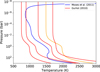 |
Fig. 1 TP-profiles used to understand temperature dependencies of sulphur-bearing species. When analysing the C/O ratio and metallicity dependence of H2S, we mainly consider the orange profile. Similarly for SO2, we mainly consider the blue TP-profile. |
2.2 Modelling the synthetic spectra
Having obtained mixing ratios using VULCAN, we used the ARCiS modelling framework (Ormel & Min 2019; Min et al. 2020) to create transmission spectra based on these mixing ratios. Within ARCiS we again used standard values for the planetary parameters of HD 189733 b. ARCiS uses correlated k-tables to create transmission spectra at low spectral resolutions (R ≤ 1000). We focused on a wavelength range of 1–10 μm. We had opacity data for 26 of the 87 species incorporated in the VULCAN C-H-N-O-S network. The correlated-k data were all taken from the ExoMolOP database (Chubb et al. 2021). These data included the most abundant and relevant species, with the exception of SO. We discuss the effect of not being able to include SO in Sect. 5.
To determine the detectability of a species, we considered the difference between transmission spectra including and excluding the relevant species. For each species we first analysed the entire wavelength range to determine at which wavelength the difference between the spectra was the largest. Simulations with different parameters were compared for the specific wavelength bin at which the difference was generally the largest: 3.78 μm for H2S and 7.26 μm for SO2. The difference between the spectrum with the species and without it is expressed in parts per million of the stellar flux. We refer to this difference as the detectability. We acknowledge that this does not truly reflect how likely it is to retrieve species from transmission spectra, since it ignores other possible sources of high opacity at this wavelength and the effect of the opacity at other wavelengths, as well as other reasons. We leave in-depth analysis using retrieval methods for specific planets to a future study.
Values for the parameters used to create the temperature-pressure profiles using the method of Guillot (2010).
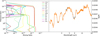 |
Fig. 2 Mixing ratios for the most relevant species (left) and transmission spectrum (right) with and without H2S. The model parameters are given in Table 1. |
3 General results
We start out by discussing the resulting transmission spectrum for our standard model (parameters given in Table 1), and assuming solar abundances for the elements. Figure 2 shows mixing ratios of the most relevant species for this study for solar abundances and the temperature profile of HD 189733 b. At the highest pressures, most carbon is stored in CH4. This changes around 101 bar, with most carbon being stored in CO at lower pressures, with a large part of the remaining oxygen being stored in H2O, which shows similar abundances to CO, due to the C/O ratio being close to 0.5. H2S is by far the most abundant sulphur-bearing species. This result is consistent across all tested metallicities, C/O ratios, and temperatures.
Figure 2 also shows the effect H2S has on the transmission spectrum, by comparing transmission spectra with and without considering H2S. This effect is quite small, peaking at 14 ppm. The difference is small, because H2S is obscured by other species, mainly H2O and HCN. The opacities of these species are shown in simplified form in Fig. 3. This illustrates the two main requirements for being able to detect a species: (i) a high enough mixing ratio to have an effect on the transmission spectrum at a specific wavelength, and (ii) not having other species competing at this wavelength. Species located higher in the atmosphere are less likely to be obscured, since they do not compete with those lower in the atmosphere. Species located lower in the atmosphere, such as H2S in this case, can still be detected, as long as other species in the atmosphere do not compete at the relevant wavelength.
We now consider CS, H2S, NS, SH, and SO2, the sulphur-bearing species for which we have opacity data. We analyse their detectability for six different TP-profiles, shown in Fig. 1, and a wide range of C/O ratios and metallicities.
3.1 NS
NS can become the main sulphur reservoir at pressures between 10−5 and 10−3 bar for colder planets with an equilibrium temperature between 750 and 1000 K, although this does require a diffusion coefficient of 1011 cm2 s−1. 750 K is the lowest temperature we considered, so we do not know how it behaves at lower temperatures. This does not lead to NS being detectable, even with such strong diffusion, due to its low opacity and the opacity being highest between a wavelength of 8 and 9 μm. At this wavelength C2H2, NH3, HCN, and CH4 also have a high opacity, leading to NS being obscured.
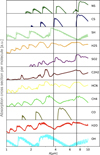 |
Fig. 3 Opacities of relevant species for a pressure of 1 bar and a temperature of 1000 K, averaged over the values of the correlated k-tables. The black lines indicate 3.78 and 7.26 μm, the wavelengths at which we analyse the detectability of H2S and SO2, respectively. |
3.2 CS
Similarly, CS can also become the main sulphur reservoir, although this happens at lower pressures than for NS, between 10−6 and 10−4 bar; in this case, for planets with an equilibrium temperature of about 900 K for solar elemental abundances. Again, just as for NS, this only happens for diffusion coefficients of at least 1011 cm2 s−1. For extremely carbon-enriched atmospheres, CS thrives at higher temperatures, with it being the main sulphur reservoir between 10−6 and 10−1 bar. CS detection suffers the same problems as NS, with a slightly higher, but still low, opacity, with the opacity being greatest near 8 μm. In the carbon-enriched, high-temperature case, CS is obscured at this wavelength by C2H2 and CH4.
3.3 SH
The mixing ratio of the third species we consider, SH, is very dependent on the mixing ratio of H2S. It is only ever the main sulphur reservoir for a very specific pressure range, at pressures lower than the pressure at which H2S becomes less abundant, at around 10−3 bar. For higher temperatures this happens slightly higher in the atmosphere. This is in agreement with previous studies into sulphur chemistry (Zahnle et al. 2009; Wang et al. 2017; Hobbs et al. 2021; Tsai et al. 2021). The opacity of SH is highest just below 4 μm, similar to H2S, with a similar value. Since H2S is significantly more abundant, it will always be easier to detect at this wavelength. As SH shows no other strong opacity features between 1 and 10 μm, we do not further consider it in our analysis.
3.4 H2S
As mentioned before, H2S is the main sulphur reservoir below 10−3 bar, with nearly all sulphur being in the form of H2S across all tested temperatures from an equilibrium temperature of 750 to 1700 K. Just as for SH, this is in full agreement with previous studies (Zahnle et al. 2009; Wang et al. 2017; Hobbs et al. 2021; Tsai et al. 2021). Since the abundance of H2S is almost entirely dependent on the abundance of sulphur, and is almost entirely independent temperature and the C/O ratio, its detectability is largely determined by the abundance of other species that can obscure it higher up in the atmosphere.
H2S has a high opacity for a wide range of wavelengths (Fig. 3), but the opacity near 3.8 μm turns out to be the most relevant, due to H2S being obscured at most other wavelengths. For most temperatures and C/O ratios, H2S is largely obscured, but for equilibrium temperatures between 1250 and 1700 K, an interesting effect can be observed, which is shown in Fig. 4. For a C/O ratio of about 0.9, the chemistry of the atmosphere begins to switch from being O–rich to C-rich, and this is reflected in the overall shape of the transmission spectrum. In particular, we can very clearly see the effect of H2S on the transmission spectrum. At this C/O ratio, almost all carbon and oxygen is stored in CO, which has a very low opacity at the relevant wavelength of 3.8 μm. For a higher C/O ratio, C2H2 and HCN become more abundant, obscuring H2S. Lower C/O ratios cause H2O to become more abundant, which also obscures H2S, although its opacity is lower than that of C2H2 and HCN near 3.8 μm. This effect is elaborated on in Sect. 4.
3.5 SO2
Similar to CS and NS, SO2 is abundant between 10−6 and 10−3 bar, although almost always less abundant than or just as abundant as SO, for which we do not have opacity data. SO2 is most abundant at equilibrium temperatures between 900 and 1000 K. Since SO2 is expected to be located higher in the atmosphere than H2S, it is less likely to be obscured, leading to its detectability being mostly dependent on its abundance alone. This is strengthened by the fact that the opacity of SO2 is highest between 7 and 8 μm, a wavelength at which most species show low opacities.
We again observe an interesting effect: whereas the abundance of H2S is extremely independent of the abundance of the elements besides sulphur, this is not the case for the SO2 abundance. Lower C/O ratios and higher metallicities both lead to an increase in the abundance of SO2. For lower C/O ratios, this can be explained by an increase in the available oxygen, with the rest being stored in CO and CO2. This effect is shown in Fig. 5. Similar to how more available oxygen leads to a higher SO2 abundance, a higher metallicity has the same effect, providing more sulphur and oxygen, which leads to a higher abundance of SO2. Naively one might expect the abundance of SO2 to be proportional to the elemental abundance of sulphur and oxygen, but it turns out the effect is significantly stronger. This is shown in Fig. 6.
This effect is best understood by analysing the relevant reactions for SO2. At the relevant pressures and mixing ratios, the reaction SO+OH→SO2+H dominates by several orders when ignoring photodissociation, which dominates the loss of SO2. The balance between this formation and destruction determines the steady state abundance. At these low pressures, the previously discussed species no longer play a significant role, since H2S and SH do no exist with a large mixing ratio. The only important species are S, S2, and the SO and SO2 discussed here. SO is mainly created through OH+S→SO+H and through the photodissociation of SO2. SO is only lost through creating SO2 and through photodissociation. OH, vital for the creation of SO and SO2, is primarily formed through the photodissociation of H2O and through O+H2→OH+H. This explains both the metallicity and the C/O ratio dependence of the SO2 abundance. A low C/O ratio leads to a large abundance of H2O, providing more OH to produce SO and SO2. High metallicities also lead to a larger H2O abundance, while also increasing the availability of S, necessary to produce SO. In the figure we can see that the overall effect of the C/O ratio and metallicity is a lot stronger for SO2 than for SO. The SO/SO2 ratio decreases from ~50 at 10−5 bar at solar metallicity, with increased oxygen to reach the C/O ratio of 0.29, to ~ 1 for ten times solar metallicity, with the same relative increase in oxygen. Figure 7 shows an example of the mixing ratios of all the relevant species in this process. At 10−6 bar a peak in OH can be seen, which coincides with a small dip in the abundance of S and the photodissociation of H2O. At lower pressures SO2 cannot exist due to the stellar irradiation. At higher pressures, due to some photodissociation of H2O still occurring and due to vertical mixing, SO2 is also formed and mixed to higher pressures. The mixing ratio sharply decreases at 10−3 bar due to almost all available sulphur forming H2S, thus providing the upper pressure limit for SO2.
 |
Fig. 4 Illustration of the detectability of H2S around C/O = 0.9 for ten times solar metallicity. From top to bottom, C/O = 0.86, 0.96, and 1.14. The spectra on the right show the transit spectrum including or excluding H2S opacity in blue and orange, respectively. |
3.6 Summary of detectability
Summarising, we find that, of the sulphur-bearing molecular species in the atmospheres that we have studied, and for which we have opacity data, H2S and SO2 are the most likely to be detected in low-resolution (R ~ 100–1000) transmission spectra in the 1–10 μm wavelength range. In the following section, we study these two molecules in more detail.
4 In depth analysis of H2S and SO2
Having discussed why we consider H2S and SO2 to be the most interesting sulphur species for detection at low resolution at a wavelength of 1–10 μm, we continue to analyse the observed effects for these species in greater detail. The effect of the C/O ratio and metallicity on the detectability is first analysed for H2S and then for SO2.
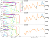 |
Fig. 5 Increased detectability of SO2 shown for ten times solar metallicity for C/O ratios of 0.23, 0.46, and 0.92 (top to bottom). |
4.1 H2S
Figure 8 shows the difference between the transmission spectra including and excluding H2S for the spectral bin centred on 3.78 μm, for a spectral resolution of 200, for a wide range of metallicities and C/O ratios. As mentioned before, this value near 3.8 μm was chosen since, in most cases, this shows the largest difference between the two spectra, while also clearly showcasing the effect. Of course H2S can also have a high detectability for different wavelengths, especially near C/O ~ 0.9, as can be seen in Fig. 4. As Fig. 8 shows, the detectability increases for an increasing C/O ratio until it peaks and then quickly decreases. This is caused, first by the H2O abundance decreasing, and after the peak of the abundance of C2H2 and HCN increasing. What can also be seen is that the peak is slightly metallicity dependent, moving to higher C/O ratios for an increase in metallicity. The actual value of this peak is only slightly metallicity dependent, which can be explained via the behaviour of H2S. Low in the atmosphere, almost all sulphur is stored in H2S, completely blocking all light at a wavelength of 3.8 μm, and an increase in metallicity only has a small effect on the impact of H2S on the transmission spectrum.
The detectability peaks at a value of 314 ppm for the case where the oxygen abundance is varied. The change in the C/O ratio is achieved by either changing the abundance of carbon or oxygen. Both achieve a very similar result, showing that the effect is mainly dependent on the C/O ratio, and not just the abundance of carbon or oxygen. Knowing this, as done in previous plots, from now on we only show results achieved by varying the abundance of oxygen.
4.2 SO2
Figure 9 shows the difference between the transmission spectra including and excluding SO2 for a bin centred on 7.26 μm, for a spectral resolution of 100, for a wide range of metallicities and C/O ratios. This wavelength was chosen because the difference between the transmission spectra is largest here for most simulations, while it only differs by a few percent in the cases where it is not. This shows the same effect described in the previous section. The overall detectability of SO2 is higher for low C/O ratios and high metallicities. At C/O ratios near one, the SO2 abundance is never high enough for it to be detectable, since almost all oxygen will be stored in CO. Similarly, for solar metallicities, detecting SO2 is not possible, with the effect on the transmission spectrum not exceeding 10 ppm. This is the result of what was described in the previous section, detailing the relation between the abundance of SO2, the abundance of species reacting to form SO2, and the effect metallicity has on these abundances.
At the highest metallicities and lowest C/O ratios, some irregularities can be observed that do not follow the expected pattern. These can be explained by the maximum effect of SO2 on the transmission being reached, with all light at 7.26 μm in the relevant pressure range being blocked. Higher SO2 abundances no longer have an effect on the transmission spectra when this is the case. At this point, slight increases in the abundances of other species can have a small effect on the detectability, due to the way we derived this value, whereas normally these small changes would not be noticeable due to the increased effect that SO2 has on the spectrum. The detectability peaks at a value of 341 ppm when varying the oxygen abundance. Similar to the situation for H2S, we again observe little difference between the contour plots derived using either a variation in carbon or oxygen to achieve the desired C/O ratio, showing that the C/O ratio is more relevant than the abundance of oxygen or carbon individually. As done up until this point, and as decided on for H2S, from now on we only show results in which the C/O ratio was achieved by varying the abundance of oxygen.
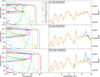 |
Fig. 6 Increased detectability of SO2 shown for a C/O ratio of 0.29 and a metallicity of one, five, and ten times solar. |
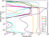 |
Fig. 7 Mixing ratios of the main species relevant for SO2 creation for a C/O ratio of 0.29 and ten times solar metallicity. |
5 Discussion
5.1 Temperature dependence
For both H2S and SO2, we have only considered a single TP-profile for each of them up to this point. To analyse the temperature dependence of the observed effects, we performed additional simulations on TP-profiles with atmospheres 200 K colder and hotter for all pressures. The results derived from this are shown in Figs. 10 and 11.
For H2S we observe that the main structure is preserved in both cases. An increase in the C/O ratio still leads to an increase in detectability, until a metallicity dependent turning-point, where the detectability falls off. Differences can be seen in the sharpness and overall height of the detectability peak. For the colder TP-profile, the peak is a lot lower, peaking at 200 ppm, and the peak is more spread out overall to lower C/O ratios. For the hotter TP-profile, the peak is a lot sharper, with a significantly lower detectability for lower C/O ratios, while the detectability peaks higher than for the original TP-profile, at 370 ppm.
For SO2 we observe that lowering the temperature leads to a significantly lower detectability. This is caused by an increase in the abundance of HCN. For this colder TP-profile, the detectability peaks at 202 ppm. For the increased temperature, we do see that the overall shape of the original is retained, although the values are slightly lower overall, leading to a maximum detectability of 300 ppm. For both species the overall characteristics seem to be retained within their 400 K window.
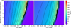 |
Fig. 8 Difference between the transmission spectra with and without H2S for the wavelength bin centred on 3.78 μm as a function of metallicity and C/O ratio. This difference gives the detectability as described in Sect. 2.2. We varied the C/O ratio by changing the oxygen (left) and carbon (right) abundance. |
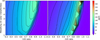 |
Fig. 10 Contour plot of H2S detectability, similar to Fig. 8, for the two TP-profiles changed to be 200 K colder (left) or hotter (right) for all pressures. In both cases the C/O ratio was varied by changing the oxygen abundance. |
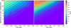 |
Fig. 11 Contour plot of SO2 detectability, similar to Fig. 9, for two TP-profiles changed to be 200 K colder (left) or hotter (right) for all pressures. In both cases the C/O ratio was varied by changing the oxygen abundance. |
5.2 Clouds
The inclusion of clouds and hazes is out of the scope of this work. Nevertheless, we note that we do not consider clouds to be a problem for detecting SO2 because of the low pressures at which it is abundant. Clouds at pressures above 10−3 bar do not impact the detectability of SO2, under the assumption that these clouds do not influence other atmospheric processes. For the detection of H2S, complete cloud coverage at these pressures would cause a big problem, almost completely removing all effects of H2S on the transmission spectrum. Complete cloud coverage above 10−2 bar halves the detectability of H2S on average, with complete cloud coverage above 10−3 bar reducing detectability to less than 10 percent. To make definitive statements about the detectability of H2S, the likelihood of clouds needs to be considered for each case.
5.3 The effect of the stellar flux
In this paper we study the chemistry and detectability of sulphur-bearing species, assuming the planetary and host-star parameters of HD 189733 b as our fiducial case. Nevertheless, to consider the effect of the stellar flux on the photochemistry and detectability of H2S and SO2, we varied the orbital radius within VULCAN. For H2S, reducing the orbital radius by half led to a maximum loss of 5 percent in detectability for the relevant C/O ratios and metallicities with respect to the original analysis. The parametrised TP-profile was significantly hotter than expected for HD 189733 b, but this illustrates how the results vary little if the planet is located at a more reasonable distance for the used TP-profile. Halving or doubling the distance also only leads to a decrease of 5 percent in detectability at worst for SO2 as well, although it can lead to small increases in certain situations. This result is quite interesting, since the creation of SO2 is directly related to photodissociation. This change in orbital radius has very little impact on this. We find that the H2O photodissociation and OH creation front shift only by a small amount, to higher or lower pressures, as a result of decreasing or increasing the orbital radius, respectively. The increase in photodissociation from a decreased orbital radius provides more OH through the photodissociation of H2O, forming SO2 in larger amounts. This seems to be balanced out by the increased photodissociation of the SO2 itself, although we have not been able to study this in detail.
We have also analysed the SO2 detectability with regards to the stellar spectrum. In addition to our original spectrum for HD 189733 from Moses et al. (2011), we also tested photospheric fits for HD 189733, and HD 209458, the latter being a significantly hotter star. To create an additional spectrum, we took the difference between our original stellar spectrum and the photospheric fit for HD 189733, and added this difference to the photospheric fit of HD 209458.
Compared to the original spectrum, detectability was found to be half in some cases when the spectrum of HD 209458 was used. Detectability decreased most when the original detectability was already low, while detectability decreased by as little as 10 percent in cases where the original SO2 detectability was high. A more detailed study of the impact of the stellar spectral shape is required to assess its full impact on SO2 detectability.
5.4 Eddy diffusion coefficient
Within the model, we chose a constant value of 109 cm2 s−1 for the diffusion coefficient. This was done to simplify the situation within reasonable bounds. It is difficult to reach convergence for extremely small or large diffusion coefficients within VULCAN, but here we analyse the effect of decreasing the diffusion coefficient to 108 cm2 s−1 and of increasing the diffusion coefficient to 1011 cm2 s−1. Lowering the diffusion coefficient to 108 cm2 s−1 has little effect on the mixing ratios for models associated with either H2S or SO2 detection. This is in agreement with Hobbs et al. (2021), who showed similar results for diffusion coefficients of 106 and 109 cm2 s−1. For H2S the detectability can decrease or increase by a few percent, with the overall detectability increasing slightly. For SO2 the detectability increases for all situations, by up to 10 percent. The effect of increasing the diffusion coefficient to 1011 cm2 s−1 is significantly bigger. Many species become significantly more abundant at low pressure, including C2H2, HCN, and H2O, which can obscure H2S, while the abundance of H2S is barely affected at all. As a result the detectability of H2S decreases by up to 30 percent, although the decrease is smaller in most cases.
SO2 is not obscured, both due to it being located higher in the atmosphere and due it not being contested by other species at the relevant wavelengths. Instead for SO2, its abundance is directly affected by the diffusion coefficient. The abundance of SO2 drastically decreases for this higher diffusion coefficient. The SO/SO2 ratio increases, with the abundance of SO being affected significantly less. Tsai et al. (2021) similarly found that the effect of SO2 on transmission spectra was significantly higher in the case of weak mixing compared to strong mixing for a model of GJ 436b. The decrease in SO2 seems to be caused by photodissociation happening higher in the atmosphere, which results in OH being formed at lower pressures. At these pressures SO is significantly less abundant, making the formation of SO2 less likely. This leads to decreases in detectability of up to 80 percent. The overall effect on the mixing ratios for H2S and SO2 are shown in Figs. 12 and 13, respectively.
5.5 SO opacity
As mentioned before, we do not have opacity data for SO. While this limits our analysis by making it hard to predict anything regarding SO detection, we do not believe this has a significant negative impact on the detectability of other sulphur-bearing species. SO does not appear in large enough abundances to obscure H2S in most scenarios, especially for the high C/O ratios where H2S detectability is greatest. Including the opacity of SO could impact SO2 detectability if it competes with it at the relevant wavelengths. In that case the overall detectability of SO+SO2 would be larger than that of SO2 alone, but it would be difficult to make statements about their individual abundances. If SO does not compete with SO2 at 7–8 μm, it could still be observed at other wavelengths. It could also be obscured, but this is unlikely due to the low pressures at which we expect SO to be abundant. In this case any detection of SO will only aid the overall understanding of the content of hot Jupiter atmospheres and provide estimates of the SO/SO2 ratio, which can also provide insight into SO2 behaviour, as mentioned previously.
5.6 Implications for planetary formation scenarios
Using our findings we can compare them to what we expect for C/O ratios and metallicities from planet formation models. We note that within these models, metallicity refers to the abundance of elements heavier than helium, whereas until now we have used metallicity as a shorthand to refer to solar abundances, with the abundance of heavier elements scaled by a certain factor. SimAb (Khorshid et al. 2022) is a basic planet formation model incorporating gas and planetesimal accretion. The contents of gas and solids are dependent on the temperature at any given orbital radius, and the input parameters of dust grain fraction and the planetesimal ratio largely determine the resulting C/O ratios and metallicities. The study finds that C/O ratios of 0.8 can be reached in extreme cases with sub-solar metallicities, while for super-solar metallicities, the possible C/O ratios range from 0.2 to 0.65.
Putting the detection limit for a planet and central star similar to HD 189733 b at 100 ppm, this leaves a small range of possible C/O ratios and metallicities for detecting H2S near a C/O ratio of 0.6 and solar metallicities. Since we do not have data for sub-solar metallicities, we cannot make predictions for H2S detection in that region, even though the C/O ratio can be significantly higher in those cases.
Using the same detection limit of 100 ppm for SO2, the range of C/O ratios and metallicities for which SO2 is detectable is significantly larger, with both C/O ratios below 0.4, with a metallicity of five times solar being detectable and C/O ratios until 0.5 reaching 100 ppm for metallicities above seven times solar. We have so far assumed that these metallicities, defined using the abundance of heavy elements, are equivalent to our previous definition of metallicity, using solar abundances, when analysing the detectability. In general, this cannot be assumed, but since we also used the associated C/O ratio, and since sulphur is found to be overabundant compared to other elements at supersolar metallicities, we believe this to be a fair comparison. Additionally, putting the detection limit at 100 ppm is very strict, leaving room for variance as a result of the differences between abundances from the different definitions of metallicity.
Another planet formation model (Turrini et al. 2021) uses n-body simulations of growing and migrating planets in planetesimal disks to find elemental abundances for carbon, nitrogen, oxygen, and sulphur for six formation scenarios that differ by their initial core position. The C/O ratio varies very little from 0.49 to 0.58. The metallicity ranges from close to solar, for an initial core position of 5 AU, to roughly eight times solar, for an initial core position of 130 AU. The relative abundances of carbon, oxygen, and sulphur remain very close to solar, with only nitrogen becoming relatively less abundant for higher metallicities. As a result, we are again confident that we can compare this to our results, even though there is a discrepancy between the two definitions of metallicity. In none of the six formation scenarios do we predict detections of H2S with the limit of 100 ppm. For detections of SO2, the limit is only reached for scenario 6 with an initial core position of 130 AU. Neither model incorporates atmospheric evolution, which could lead to a wider range of possible atmospheric compositions.
 |
Fig. 12 Comparison of the effect of a diffusion coefficient of 108, 109, and 1011 cm2 s−1 on mixing ratios for ten times solar metallicity, a C/O ratio of 0.96, and the TP-profile associated with H2S detection. |
 |
Fig. 13 Comparison of the effect of a diffusion coefficient of 108, 109, and 1011 cm2 s−1 on mixing ratios for ten times solar metallicity, a C/O ratio of 0.29, and the TP-profile associated with SO2 detection. |
6 Conclusions
In this work we analyse the detectability of sulphur-bearing species in hot Jupiter atmospheres. To achieve this, we used the ID open-source photochemical kinetics code VULCAN to simulate such atmospheres. Low-resolution transmission spectra were created using the modelling framework ARCiS based on the output of VULCAN. These results were placed into context by further analysing the dependence on temperature, cloud formation, the diffusion coefficient, and planet formation models.
We find that H2S and SO2 are the sulphur-bearing species most likely to be detected. H2S is found in high abundances in most cases, but its detection relies on other species not being present in excessively high abundances to obscure it. This happens at a temperature near 1500 K for C/O ratios between 0.7 and 0.9, depending on the metallicity. SO2 can be formed in high abundances at temperatures close to 1000 K and low pressures. Both low C/O ratios and high metallicities contribute to a high SO2 abundance. Due to other species not showing large opacities near 7 μm and SO2 only being found at low pressures, SO2 is unlikely to be obscured.
Results for both H2S and SO2 are relatively stable for a temperature decrease or increase of 200 K. Results also remain consistent when the eddy diffusion coefficient is decreased. Increasing the diffusion coefficient to 1011 cm2 s−1 shows a significant decrease in detectability for both H2S and SO2, although SO2 is affected more. H2S detectability can be affected by the presence of clouds, while SO2 is not affected. H2S is barely affected by a change in stellar flux, while SO2 is significant affected. The shape of the stellar spectrum is largely irrelevant, with the overall luminosity being more important. Planet formation models indicate that it is unlikely for atmospheres to have the ideal C/O ratios and metallicities for H2S detection, although detection could still be possible. SO2 is most likely easier to detect, due to planet formation models favouring the formation of low C/O ratio, high-metallicity planets.
Acknowledgements
We gratefully acknowledge support from the VULCAN development team. We thank the referee for useful comments and suggested additions to this paper. Y.M. and L.B.F.M. Waters are part of an international ISSI team.
References
- Cazaux, S., Carrascosa, H., Muñoz Caro, G. M., et al. 2022, A&A, 657, A100 [NASA ADS] [CrossRef] [EDP Sciences] [Google Scholar]
- Cernicharo, J., Cabezas, C., Agúndez, M., et al. 2021, A&A, 648, L3 [EDP Sciences] [Google Scholar]
- Chubb, K. L., Rocchetto, M., Yurchenko, S. N., et al. 2021, A&A, 646, A21 [NASA ADS] [CrossRef] [EDP Sciences] [Google Scholar]
- Codella, C., Bianchi, E., Podio, L., et al. 2021, A&A, 654, A52 [NASA ADS] [CrossRef] [EDP Sciences] [Google Scholar]
- Guillot, T. 2010, A&A, 520, A27 [NASA ADS] [CrossRef] [EDP Sciences] [Google Scholar]
- Hobbs, R., Rimmer, P. B., Shorttle, O., & Madhusudhan, N. 2021, MNRAS, 506, 3186 [NASA ADS] [CrossRef] [Google Scholar]
- Kama, M., Shorttle, O., Jermyn, A. S., et al. 2019, ApJ, 885, 114 [Google Scholar]
- Khorshid, N., Min, M., Désert, J.M., Woitke, P., & Dominik, C. 2022, A&A 667, A147 [NASA ADS] [CrossRef] [EDP Sciences] [Google Scholar]
- Laas, J. C., & Caselli, P. 2019, A&A, 624, A108 [NASA ADS] [CrossRef] [EDP Sciences] [Google Scholar]
- Le Gal, R., Öberg, K. I., Teague, R., et al. 2021, ApJS, 257, 12 [NASA ADS] [CrossRef] [Google Scholar]
- Lodders, K., Palme, H., & Gail, H. P. 2009, Landolt Börnstein, 4B, 712 [Google Scholar]
- Madhusudhan, N. 2019, ARA&A, 57, 617 [NASA ADS] [CrossRef] [Google Scholar]
- Min, M., Ormel, C. W., Chubb, K., Helling, C., & Kawashima, Y. 2020, A&A, 642, A28 [NASA ADS] [CrossRef] [EDP Sciences] [Google Scholar]
- Moses, J. I., Visscher, C., Fortney, J. J., et al. 2011, ApJ, 737, 15 [Google Scholar]
- Ormel, C. W., & Min, M. 2019, A&A, 622, A121 [NASA ADS] [CrossRef] [EDP Sciences] [Google Scholar]
- Tsai, S.-M., Lyons, J. R., Grosheintz, L., et al. 2017, ApJS, 228, 20 [NASA ADS] [CrossRef] [Google Scholar]
- Tsai, S.-M., Malik, M., Kitzmann, D., et al. 2021, ApJ, 923, 264 [NASA ADS] [CrossRef] [Google Scholar]
- Turrini, D., Schisano, E., Fonte, S., et al. 2021, ApJ, 909, 40 [Google Scholar]
- Wang, D., Miguel, Y., & Lunine, J. 2017, ApJ, 850, 199 [NASA ADS] [CrossRef] [Google Scholar]
- Zahnle, K., Marley, M. S., Freedman, R. S., Lodders, K., & Fortney, J. J. 2009, ApJ, 701, L20 [Google Scholar]
All Tables
Values for the parameters used to create the temperature-pressure profiles using the method of Guillot (2010).
All Figures
|
Fig. 1 TP-profiles used to understand temperature dependencies of sulphur-bearing species. When analysing the C/O ratio and metallicity dependence of H2S, we mainly consider the orange profile. Similarly for SO2, we mainly consider the blue TP-profile. |
| In the text | |
|
Fig. 2 Mixing ratios for the most relevant species (left) and transmission spectrum (right) with and without H2S. The model parameters are given in Table 1. |
| In the text | |
|
Fig. 3 Opacities of relevant species for a pressure of 1 bar and a temperature of 1000 K, averaged over the values of the correlated k-tables. The black lines indicate 3.78 and 7.26 μm, the wavelengths at which we analyse the detectability of H2S and SO2, respectively. |
| In the text | |
|
Fig. 4 Illustration of the detectability of H2S around C/O = 0.9 for ten times solar metallicity. From top to bottom, C/O = 0.86, 0.96, and 1.14. The spectra on the right show the transit spectrum including or excluding H2S opacity in blue and orange, respectively. |
| In the text | |
|
Fig. 5 Increased detectability of SO2 shown for ten times solar metallicity for C/O ratios of 0.23, 0.46, and 0.92 (top to bottom). |
| In the text | |
|
Fig. 6 Increased detectability of SO2 shown for a C/O ratio of 0.29 and a metallicity of one, five, and ten times solar. |
| In the text | |
|
Fig. 7 Mixing ratios of the main species relevant for SO2 creation for a C/O ratio of 0.29 and ten times solar metallicity. |
| In the text | |
|
Fig. 8 Difference between the transmission spectra with and without H2S for the wavelength bin centred on 3.78 μm as a function of metallicity and C/O ratio. This difference gives the detectability as described in Sect. 2.2. We varied the C/O ratio by changing the oxygen (left) and carbon (right) abundance. |
| In the text | |
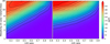 |
Fig. 9 Same as for Fig. 8, but for SO2, using the 7.26 um spectral region. |
| In the text | |
|
Fig. 10 Contour plot of H2S detectability, similar to Fig. 8, for the two TP-profiles changed to be 200 K colder (left) or hotter (right) for all pressures. In both cases the C/O ratio was varied by changing the oxygen abundance. |
| In the text | |
|
Fig. 11 Contour plot of SO2 detectability, similar to Fig. 9, for two TP-profiles changed to be 200 K colder (left) or hotter (right) for all pressures. In both cases the C/O ratio was varied by changing the oxygen abundance. |
| In the text | |
|
Fig. 12 Comparison of the effect of a diffusion coefficient of 108, 109, and 1011 cm2 s−1 on mixing ratios for ten times solar metallicity, a C/O ratio of 0.96, and the TP-profile associated with H2S detection. |
| In the text | |
|
Fig. 13 Comparison of the effect of a diffusion coefficient of 108, 109, and 1011 cm2 s−1 on mixing ratios for ten times solar metallicity, a C/O ratio of 0.29, and the TP-profile associated with SO2 detection. |
| In the text | |
Current usage metrics show cumulative count of Article Views (full-text article views including HTML views, PDF and ePub downloads, according to the available data) and Abstracts Views on Vision4Press platform.
Data correspond to usage on the plateform after 2015. The current usage metrics is available 48-96 hours after online publication and is updated daily on week days.
Initial download of the metrics may take a while.