| Issue |
A&A
Volume 693, January 2025
|
|
|---|---|---|
| Article Number | A177 | |
| Number of page(s) | 13 | |
| Section | Numerical methods and codes | |
| DOI | https://doi.org/10.1051/0004-6361/202450383 | |
| Published online | 15 January 2025 | |
Hydrodynamical simulations with strong indirect terms in FARGO-like codes
Numerical aspects of the non-inertial frame and artificial viscosity
1
Institut für Astronomie und Astrophysik, Universität Tübingen,
Auf der Morgenstelle 10,
72076
Tübingen,
Germany
2
Zentrum für Astronomie (ZAH), Institut für Theoretische Astrophysik (ITA), Universität Heidelberg,
Albert-Ueberle-Str. 2,
69120
Heidelberg,
Germany
★ Corresponding author; This email address is being protected from spambots. You need JavaScript enabled to view it.
Received:
15
April
2024
Accepted:
26
November
2024
Abstract
Context. Binary star systems allow us to study the planet formation process under extreme conditions. In the early stages, these systems contain a circumbinary disk and a disk around each star. To model the interactions between these disks in the frame of one of the stars, strong fictitious forces must be included in the simulations. The original FARGO and the FARGO3D codes fail to correctly simulate such systems if the indirect term becomes too strong.
Aims. We present a different way to compute the indirect term that, together with a tensor artificial viscosity prescription, allows the FARGO code to simulate the circumbinary disks in a non-inertial frame of reference. In this way, the FARGO code can be used to study interactions between circumstellar and circumbinary disks.
Methods. We first evaluated the accuracy of the standard implementation and our proposed indirect term prescription using a simple N-body test case. We then analytically estimated the effect of the default artificial viscosity used in the FARGO code in the limit of large distances to the N-body system. Finally, we evaluated the effects of the different prescriptions by performing hydrodynamical simulations in a non-inertial frame of reference.
Results. By updating the indirect term prescription and the artificial viscosity, we were able to successfully simulate a circumbinary disk in a frame that is centered on the less massive star. We find that updating the indirect term becomes relevant when the indirect term becomes stronger than the direct gravitational forces, which occurs for mass ratios of q ≳ 5%. The default artificial viscosity used in the FARGO code inherently produces artificial pressure in a non-inertial frame of reference even in the absence of shocks. This leads to artificial mass ejection from the Hill sphere, starting at brown dwarf masses (q ≳ 1%). These problems can be mitigated by using a tensor artificial viscosity formulation. For high mass ratios, q ≳ 1%, it is also becomes important to initialize the disk in the center-of-mass frame. We expect our proposed changes to be relevant for other grid-based hydrodynamic codes where strong indirect terms occur, or for codes that use artificial viscosity.
Key words: accretion, accretion disks / hydrodynamics / methods: numerical / protoplanetary disks / planet-disk interactions / binaries: general
© The Authors 2025
 Open Access article, published by EDP Sciences, under the terms of the Creative Commons Attribution License (https://creativecommons.org/licenses/by/4.0), which permits unrestricted use, distribution, and reproduction in any medium, provided the original work is properly cited.
This article is published in open access under the Subscribe to Open model. This email address is being protected from spambots. You need JavaScript enabled to view it. to support open access publication.
1 Introduction
When studying astrophysical hydrodynamics simulations, it is of interest to conduct such studies in a non-inertial frame of reference, that is to center the simulation on one star of a binary system to study its circumstellar disk. The non-inertial frame of reference introduces fictitious forces that must be taken into account in the simulation.
The indirect term is supposed to compensate for the forces acting on the center of the frame of reference so that it does not move. In extreme cases, the force due to the indirect term dominates the total force acting on the gas. Under such conditions, an overly simplistic approach for handling the indirect term can become the limiting factor in the accuracy of the entire simulation.
In this paper, we discuss the artificial viscosity and the indirect term used in the FARGO and FARGO3D codes (Masset 2000; Benítez-Llambay & Masset 2016) and show that they cause problems when simulating extreme setups. We then propose a more accurate method for handling the indirect term and the use of the tensor artificial viscosity by Tscharnuter & Winkler (1979) and show that they are more accurate at simulating systems with strong indirect terms. The methods presented in this paper have already been mentioned in Rometsch et al. (2024). In this paper, we explain the methods in detail and explore when they become necessary.
In Sect. 2 we compare two strategies for calculating the indirect term in a binary star system by testing how well the primary component of the binary remains fixed in a reference frame centered on the primary. We discuss two forms of artificial viscosity that are commonly used in grid codes in Sect. 3, and then use the proposed changes to run hydrodynamical simulations with strong indirect terms in Sect. 4. We then evaluate the relevance of our modifications to planetary disk simulations in Sect. 5 and discuss our results in Sect. 6.
2 N-body example on applying the indirect term
In the FARGO and FARGO3D codes, the indirect term is calculated at the beginning of the time step and then added to the potential that is then derived numerically to calculate the acceleration on the gas. Next, the source terms due to pressure, viscosity, and artificial viscosity and, finally, the transport step are calculated and applied.
In this section, we construct a pure N-body test case where only gravitational forces are considered, using the REBOUND code (Rein & Liu 2012). This is a model of the full action to study the effects of different protocols for including the indirect term.
We initialized a binary star system in REBOUND and shifted it into the frame of the primary star. We then updated the velocities of the N -body in time with the indirect term using a forward Euler step in time before applying the standard REBOUND integration step. We used the IAS15 integrator (Rein & Spiegel 2015) that is accurate to machine precision. We therefore assumed that any motion of the central object is due to inaccuracies in the indirect term protocols. This allowed us to measure their quality by how little the central object moves.
For a binary star system with masses m1, m2 and positions x1, x2, the indirect term is simply given by the negative of the acceleration of the primary by the secondary:
 (1)
(1)
This formulation is identical to the implementation in the FARGO code. We call it the Euler protocol because the velocity update is similar to a Euler integrator in the sense that it updates the velocity with a single step forward in time using the positions at the beginning of a time step.
As an alternative, we propose to use the acceleration experienced by the primary during its entire update step to compute the indirect term. In our case, we extracted the acceleration on the central object from the REBOUND code by measuring the change in velocity during the entire integration step:
 (2)
(2)
where Δt is the size of the time step and v1 (t) is the velocity of the central object at the time t. To obtain the indirect term at the beginning of the time step, we created a copy of the N -body system and then integrated the copy with all the external forces acting on it to compute the accelerations. Assuming that the velocity of the central object at the start of the time step is zero, which is satisfied in a frame centered on it, Eq. (2) simply represents a velocity shift to the frame of the central object. For this reason, we call this method the shift protocol for the indirect term. We also computed the acceleration using a fifthorder Runge–Kutta scheme and found identical results up to the accuracy of the integration scheme.
For our test, we used a circular binary system with a mass ratio of m2/m1 = 0.1 and chose the units so that the total mass, binary separation, and gravitational constant are all equal to one. With this setup, one binary period is Pbin = 2π that is divided into 250 steps Δt = 2π/250 for integration. The primary star was initially placed in the coordinate center.
The time evolution of the primary star in simulations using the Euler and shift protocols for considering the indirect term are shown in Fig. 1. Neither implementation keeps the primary fixed at x = 0. For the shift protocol, the velocity is zero at the end of each time step, and the primary drifts on a circle. For the Euler protocol, the primary reaches zero velocity only after each full binary orbit and moves away from the origin. By design, the shift protocol keeps the primary at zero velocity. Any motion is only due to drift during the integration step as the primary is accelerated from −ΔtaInd,2 to 0.
For the next test, we shifted the binary system into the primary frame at the end of each time step to fix the primary at the coordinate center. This is intended to simulate the implementation of the FARGO codes in which the central object is implicit; in other words, the central object is not integrated, and the other N -body objects feel the indirect term at each substep of a fifthorder scheme, so that they are held in the frame of the central object with high accuracy.
We then added massless test particles that were integrated alongside the binary. Their velocities were updated with the indirect term at the beginning of the time step by adding aInd Δt, but were not shifted into the primary frame at the end of each time step. They represent gas cells on a fixed grid and therefore cannot be shifted to the primary frame. We also added a test particle that is shifted to the primary frame along with the binary after each time step as a reference. We modeled the time step criteria of a hydrocode by scaling the time step by the inverse velocity of the innermost particle, normalized by the Kepler velocity for a circular orbit at the same semi-major axis:
 (3)
(3)
which mimics the CFL criteria of the FARGO code.
The resulting evolution of the semi-major axis and eccentricity for test particles starting at 3, 4, 20 abin are shown in Fig. 2. The first three rows correspond to a different initial semi-major axis, a0 , and the bottom row shows a zoom in for the case of a0 = 20 abin . The left and right columns of the panels show the semi-major axis, a, of the test particles and their eccentricity, e, as a function of time, respectively. We note that the two columns show the quantities over different time frames.
In total, we identified four different oscillations in the particle orbits. The first has a period equal to the synodic period of the binary. They can be seen in the semi-major axis evolution of the innermost particle starting at 3 abin in the upper-left panel in Fig. 2. They are characterized by their double peaks and valleys during a binary period as the particles move through the potential of the binary. This oscillation is always present for the reference particle and is visible in the semi-major axis and eccentricity. In the simulations with an indirect term, this oscillation is dominated by other oscillations and is no longer visible at larger radii.
The second oscillation has a frequency of the orbital period of the particles. This oscillation occurs only in the eccentricity of the particles, and it is clearly visible in the lower-right panel. For reference, the particles at 20 abin have a period of ≈90 Pbin .
In addition to these two physical oscillations, we find two purely numerical oscillations for the particles with an indirect term, which do not occur for the reference particle. The first numerical oscillation also has a period equal to the synodic period of the binary, but produces only a single peak and valley instead of the two for the oscillation due to the binary potential. We associate this oscillation with the residual motion due to the indirect term protocols, similar to those shown in Fig. 1 for the central object. Examples of this oscillation can be seen in the semi-major axis evolution of the particles starting at 20 abin (third and fourth panels on the left in Fig. 2). They also appear in the eccentricity of the particles, but cannot be seen individually because the eccentricity plots cover a larger time frame.
Finally, in simulations with indirect terms, the outer particles also oscillate due to the feedback from the time-stepping criteria that is calculated from the velocity of the innermost particle (see Eq. (3)). The frequency of this oscillation is the beat frequency between the orbital frequency of the particle itself and the innermost particle. This CFL oscillation causes the height of the peaks and valleys to oscillate during the synodic period, as seen in the semi-major axis and eccentricity for particles starting at 4 abin and 20 abin .
In addition to the oscillations, we observe other differences between the reference particles and the particles subject to an indirect term. For the Euler protocol, the innermost particle (top row of Fig. 2) drifts inward, and its eccentricity increases. For the shift protocol, the particle drifts outward at one-third the drift of the of the Euler protocol particle, and its eccentricity does not increase. The sign of the drift direction and the sign of the deviations from the reference particle in general, are reversed by applying the indirect term after the integration step instead of before. The drift of the innermost particles is caused by the variable time step and does not occur with a constant time step.
The second row shows the time evolution of the second particle that started at a distance of 4 abin . The particles subject to the indirect terms are no longer drifting. At t = 150 Pbin the time step variations induce an eccentricity growth in the simulation using the Euler protocol. We ran an additional simulation where the time step from the Euler protocol simulation was copied and used for the outer particle with the shift-based protocol starting at 4 abin (not shown), which also caused it to increase its eccentricity, but at half the rate of the case where both particles used the Euler protocol.
The third row shows the particle at a distance of 20 bin, and the fourth row shows the same data again, but without the particle affected by the Euler protocol. For the Euler protocol, the eccentricity is higher by a factor of 35 and oscillates at twice the rate of its binary period. The eccentricity of the shift protocol particle has the oscillation with its binary period as the dominant oscillation and still resembles the time evolution of the reference particle. We repeated the test and measured the amplitudes of the oscillations in the semi-major axis of the outer test particle for different binary mass ratios, time step sizes, and initial semi-major axes.
An example of how we measured the oscillation amplitudes is shown in the third panel on the left in Fig. 2. We measured the amplitude of the combined physical and shift protocol oscillations during the synodic period, Asyn, as the differences between the maxima (blue dots) and the subsequent minima (red crosses) of the semi-major axis. We defined the amplitude of the oscillations due to the CFL criteria, ACFL , as the difference between the highest and lowest maximum of the semi-major axis, as indicated by the purple and yellow dots. The amplitudes were always measured during the first 30 binary orbits, so that the particles were still close to their initial positions. We ignored the numerical drift and used the initial semi-major axis of the particle for the evaluation. The initial semi-major axis of the particle used for the time step criteria was kept at 3 abin, while the other particle was varied from 2.5 to 28 abin. The resulting amplitudes for the different indirect term protocols as a function of the initial semi-major axis are given in Fig. 3.
We evaluated the trends of the amplitudes by fitting a power law model to the data of the form:
 (4)
(4)
where a0 is the initial semi-major axis of the particle, q = m2/m1 is the mass ratio of the binary, and Δt is the time step size. The power law indices ni were fixed to the values in Table 1, while the constant A0 and the coefficients ci were determined by a least squares fit. For all fitted parameters, we find relative 2σ errors of less than 11% that we interpret as confirmation of the power law indices given in Table 1. The fits for the radial dependencies are plotted in Fig. 3 as dashed lines. The other power law dependencies for time step and binary mass ratio were determined in the same way.
For both indirect term protocols, we find oscillation amplitudes that scale linearly with the time step size, as expected from a first-order method. The amplitudes of the synodic oscillations depend linearly on the mass ratio, identical to the reference model, since they are physical and caused by the perturbations of the companion star that scale linearly with its mass. The amplitudes of the oscillations due to the CFL criteria scale with the square of the companion mass, because they depend on the strength of the perturbation as well as on the velocity variations of the innermost particle according to Eq. (3).
From the reference particles we infer that the amplitude of the synodic oscillations due to the variations in the binary potential scale with the initial semi-major axis as  . For the shift protocol, the amplitude of the synodic oscillations reaches a constant floor value at distances above 8 abin . We interpret this as the oscillations being dominated by the potential close to the binary. This causes the particle using the shift protocol to behave similarly to the reference particle at distances below 8 abin while beyond 8 abin, the numerical oscillations dominate and their behavior diverges. For the Euler protocol, the numerical oscillation amplitudes increase with
  and are already significantly larger than the reference amplitude at an initial separation of 4 abin .
For both the synodic period oscillation and the time step criteria oscillation, the magnitude of the errors of the Euler protocol at large radii is a factor of (a0/abin)1.5 larger than the errors of the shift protocol. Since a0 > abin for circumbinary particles, the errors of the Euler protocol will always be larger than the errors of the shift protocol in this case.
We repeated similar tests for particles on an s-type orbit, that is, orbiting the central object with the companion as an outside perturber. For this configuration, the indirect term will always be weaker than the direct gravitational forces. We used the same binary setup as before and put the inner particle used for the time step criteria at 0.3 abin and the outer particle at 0.5 abin. We reduced the time step so that the orbit of the inner particle was resolved with 250 steps. For this setup, both indirect term protocols induced an artificial inward drift that scales linearly with the time step size, with the shift protocol leading to a 20% faster drift than the Euler protocol. The deviations of the oscillation amplitudes from the reference particle are on the order of 10−3 and can be positive or negative depending on the time step size for both protocols. Thus, we do not find a clear trend of increasing inaccuracies as we did for the p-type orbits before.
We conclude that single-step-forward-in-time methods for the indirect term introduce inaccuracies that scale with the time step size and the strength of the indirect term. When the time step is determined by the velocity of a particle, analogous to a cell in a hydrodynamic simulation, it creates a feedback effect that causes the particle itself to migrate and induce oscillations in the other particles. We have introduced a new method for calculating the indirect term that is more accurate and stable for p-type orbits (orbits around both binary stars) than the standard indirect term protocol typically used in hydrocodes.
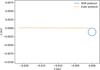 |
Fig. 1 Time evolution over three binary periods of the primary under the influence of the indirect term protocols of Eqs. (1) and (2). |
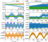 |
Fig. 2 Time evolution of the semi-major axis and eccentricity of two test particles under the influence of the indirect term in Eq. (1) and Eq. (2) respectively and an exact reference case without an indirect term. |
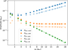 |
Fig. 3 Amplitudes of the semi-major axis oscillations as a function of the initial semi-major axis. The dotted line at 3 abin indicates the initial position of the particle that is used for the time step criteria. The dashed lines represent the best least squares fit with a power law model. |
3 Artificial viscosity
The FARGO codes use a second-order upwind scheme for the hydrodynamic advection that cannot handle discontinuities and requires artificial viscosity to spread shocks over multiple grid cells. By default, FARGO codes use the artificial viscosity developed by Von Neumann & Richtmyer (1950, hereafter VNR50), which acts as a bulk viscosity and enters the equation of motion as an anisotropic artificial pressure to counteract compression. The implementation of the artificial viscosity is described in Stone & Norman (Section 4.3 1992, hereafter SN92), who define the artificial viscosity in one dimension and apply it to each dimension independently:
 (5)
(5)
where c is the artificial viscosity constant that measures the number of cells over which the shock spreads, for which values around 2 are typically recommended, and Δxi is the cell size along direction i. We note the misprint in Eqs. (33) and (34) by SN92, where they forgot to square the artificial viscosity constant c.
Tscharnuter & Winkler (1979, hereafter TW79) raised concerns about the formulation of artificial viscosity by VNR50 being used on curve-linear coordinate systems, since it is formally valid only for Cartesian coordinates. They show that it can create artificial pressure in curve-linear coordinates even when there are no shocks. A specific example is given in Bodenheimer et al. (2006, Section 6.1.4) where they show that the artificial viscosity by VNR50 creates an artificial pressure that accelerates the collapse of a free-falling spherical gas cloud (|vr| ∝ r) even though the flow is smooth.
TW79 proposed a tensor artificial viscosity, analogous to the viscous stress tensor, which is independent of the coordinate system and frame of reference. An implementation of this artificial viscosity is also described in SN92, Appendix B, who added two additional constraints to the artificial viscosity prescription by TW79: the artificial viscosity constant must be the same in all directions (isotropy), and the off-diagonal elements of the tensor must be zero to avoid artificial angular momentum transport. The resulting artificial viscosity pressure tensor is given by:
![Mathematical equation: ${\bf{Q}} = \left\{ {\matrix{ {{c^2}\Delta {x^2}\Sigma \nabla {\bf{v}}\left[ {\nabla \otimes {\bf{v}} - {1 \over 3}\nabla {\bf{vI}}} \right]} \hfill & {{\rm{ if }}\nabla {\bf{v}} < 0,} \hfill \cr0 \hfill & {{\rm{ otherwise, }}} \hfill \cr } } \right.$](/articles/aa/full_html/2025/01/aa50383-24/aa50383-24-eq14.png) (6)
(6)
where c is again a dimensionless parameter near unity and Δx is the maximum cell extension in any direction.
We can analytically estimate the effect of the more naive approach given in Eq. (5) for a disk in a non-inertial frame. We considered the case of a Keplerian gas disk around a circular two-body system in the center-of-mass frame, where the primary moves at a velocity of v0 . If the radial velocity of the gas is neglected, the gas has the Cartesian velocity components:
 (7)
(7)
where vk is the Keplerian velocity and ϕ is the angle in the center- of-mass frame. We then shifted the whole system to the primary frame by subtracting its position and velocity from the gas and binary. After shifting to the primary center, the gas has the following velocity components:
 (8)
(8)
 (9)
(9)
where φ is the angle in the primary frame and φ0 is the azimuthal angle of the companion in the primary frame. Without loss of generality, we assumed φ0 = 0, meaning that the binary is located on the x-axis and the secondary moves in the positive y-direction in the primary frame. In addition, we made the simplifying assumption that the length of the position vector of the cell is much greater than the length of the shift vector from the center of mass to the primary, so that its angular position is the same in the center-of-mass frame and in the primary frame: ϕ ≈ φ. Under these assumptions, the velocity of the gas has no radial dependence. This causes the radial component of the artificial pressure in Eq. (5), which depends only on the radial derivatives of the radial velocity, to always be zero. Therefore, we do not consider the radial velocity any further. The azimuthal velocity becomes:
 (10)
(10)
Putting this velocity into Eq. (6) results in zero artificial viscosity, while putting it into Eq. (5) results in an artificial viscosity of:
![Mathematical equation: ${Q_\varphi } = \left\{ {\matrix{ {{c^2}\Sigma {{\left[ { - \Delta \varphi \cdot {\upsilon _0}\sin (\varphi )} \right]}^2}} \hfill & {{\rm{ if }}0 < \varphi < \pi } \hfill \cr0 \hfill & {{\rm{ if }}\pi < \varphi < 2\pi } \hfill \cr } ,} \right.$](/articles/aa/full_html/2025/01/aa50383-24/aa50383-24-eq19.png) (11)
(11)
where Δφ = 2π/Nφ is the angular cell size of the grid and Nφ is the number of azimuthal grid cells. The acceleration due to the artificial viscosity is then:
 (12)
(12)
If we use units for which GM = 1, and assume that the cell is far enough away from the two-body object that the distance to the primary at the center is approximately equal to the distance to the companion, we find the ratio of the artificial acceleration,  , to the magnitude of the direct gravitational acceleration caused by the companion, |a2|, to be:
 (13)
(13)
where q is the mass ratio of the companion to the primary and a is the semi-major axis. For typical values used in planetdisk interaction simulations with a Jupiter-mass planet, such as  , q = 10−3, r = 10 a, and Nφ = 1024, we find a ratio of the artificial acceleration to the acceleration caused by the planet of up to 7.5 ⋅ 10−7. Assuming a locally isothermal equation of state and a scale height of h = 0.05, the maximum artificial pressure due to Eq. (11) is 3 ⋅ 10−7 times the pressure of the gas.
For a circumbinary disk, this ratio becomes much larger and very relevant in the simulations. The artificial accelerations due to Eq. (13) are shown in Fig. 4 for a binary system in the frame of the secondary. The simulation parameters are the same as in Sect. 4, the binary has a mass ratio of q = 2 and an eccentricity of ebin = 0.4, the grid has Nφ = 315 azimuthal cells, and the artificial viscosity constant is  . The binary is currently in the pericenter. For the parameters of this model, our estimate for the artificial pressure using Eq. (13) predicts a force during the binary periastron passage that is 0.6% of the gravitational force of the primary at r = 5 abin, which is two-thirds of the pressure forces of the gas itself.
The left panel is zoomed in on the binary and depicts the azimuthal velocity of the gas according to Eq. (10) normalized by the Keplerian velocity. It is shown to visualize the setup and its extreme case where the velocity of the gas is dominated by the velocity of the frame. The right panel depcits the resulting acceleration field due to the SN artificial viscosity normalized by the gravitational acceleration caused by the primary (Eq. (13)). The right panel of Fig. 4 covers the same area as Fig. 5.
The depicted acceleration field rotates with the binary. Looking at a fixed cell far from the binary (with a slower orbital frequency than that of the binary) as the acceleration field rotates with the binary, the deceleration and subsequent acceleration result in an epicyclic motion with the same frequency as the orbital frequency of the binary. In a non-isothermal simulation, the artificial viscosity in Eq. (11) would be used to calculate the shock heating of the gas and the gas would be artificially heated.
If the binary is eccentric, then the accelerations during a binary orbit would not cancel each other out, instead the acceleration during the binary periastron passage would be higher than during the apastron passage. This leads to a residual acceleration field with the same shape as the one presented in Fig. 4. The deceleration and acceleration during an orbit is a similar pattern to a particle on an eccentric orbit. In this case, the artificial acceleration could excite an eccentricity with a preferred direction based on the location of the binary periastron.
A circumplanetary disk in the frame of the star will have similar problems. The circular motion around the planet will appear as radial and azimuthal velocity components oscillating around the planet in the frame of the central star. The resulting radial and azimuthal velocity gradients are treated as shocks by the artificial viscosity prescription in Eq. (5). In addition, the resolution in the vicinity of a planet on a logarithmic polar grid is typically much lower than the global resolution. We analyze the influence of the different choices of artificial viscosity on a circumplanetary disk further in Appendix A. In our tests presented in Sect. 5, we find that the disks around the companion begin to behave differently for the two artificial viscosity prescriptions at companion masses of 3 MJup(q ≥3 ⋅ 10−3).
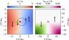 |
Fig. 4 Snapshot of the azimuthal velocity (left) and artificial acceleration due to Eq. (13) in the frame of the secondary (right). The red dot represents the secondary, the green dot represents the primary, and the black dashed line represents the orbit of the primary. The arrows indicate the direction of motion and are not to scale. The binary and grid parameters are the same as in Sect. 4. |
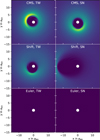 |
Fig. 5 Snapshot of the surface density after 5000 binary orbits of a massless disk around a binary system with qbin = 0.5 and ebin = 0.4. The plots show the results for different combinations of coordinate centers, artificial viscosity, and indirect term protocol. All plots use the same linear color scale. |
4 Circumbinary disk in non-inertial frame
To highlight the importance of our changes to the indirect term and the use of the artificial viscosity by TW79, we constructed a test by simulating a circumbinary disk in the center-of-mass frame and in the center of the secondary star. For all our hydro-dynamical simulations, we used the FARGOCPT code that is freely available on GitHub1 and described in detail in Rometsch et al. (2024).
The simulations are locally isothermal and we used the α viscosity prescription from Shakura & Sunyaev (1973) (α = 0.01, h = 0.04 ⋅ (d/abin)0.3, GM = 1). The surface density was initialized as Σ(d) = Σ0 ⋅ (d/abin)−1.1. The gas velocities and surface densities were always initialized in the center-of-mass frame, and d is the distance to the center of mass, which is not equal to the r coordinate of the grid in the secondary frame. The setup is intended to model a steady state accretion disk around a binary star system. The artificial viscosity constant was set to  .
.
The domain is logarithmically spaced from 1 to 60 abin in the radial direction and uniformly spaced from 0 to 2π in the azimuthal direction with a resolution of Nr × Nφ = 207 × 315, or equally, 2 cells per scale height at r = 1 abin. The resolution was chosen low to make this a stress test for the numerical scheme. The disk was damped to the initial conditions from 36 to 60 abin on a timescale of 10−3 Keplerian orbital periods at 60 abin. We applied strict outflow conditions at the inner boundary, and in case a star enters the simulation domain, we added a sink hole around each star that removes a fraction of the gas within its Roche lobe with a half-emptying time of 10−2 Torb. The removed mass was included in the accretion rate, but was not added to the mass of the stars. We used a density floor of 10−7 ⋅ Σ0 for numerical stability, meaning that if the density of a cell falls below this value, it will be set to this value. The gravity of the gas was ignored. The mass of the secondary was mSec = 0.5 and mPrim = 1 for the primary star. The binary eccentricity of ebin = 0.4 caused the primary to enter the simulation domain during its orbit when the simulation was centered on the secondary. To prevent this from causing numerical problems, we smoothed the gravitational potential of the primary within a radius of 0.5 RHill around it using the third-order polynomial prescription by Klahr & Kley (2006, Eq. (4)). To make the time step size comparable between the simulations, we used a Courant number of 0.4 in simulations using the artificial viscosity by Stone & Norman (1992) and a Courant number of 0.5 in simulations using the artificial viscosity by Tscharnuter & Winkler (1979).
We ran the setup with different combinations of coordinate centers (default is centered on the secondary and ‘CMS’ indicates the simulation is in the center-of-mass system) and artificial viscosity (“TW” is the artificial viscosity by TW79 and “SN” is the artificial viscosity by VNR50, implemented as described in SN92). The ‘CMS’ simulations are a reference case for the indirect term experiments, since the indirect term vanishes in the center-of-mass system.
Snapshots of the surface densities after 5000 Tbin are shown in Fig. 5. The top row shows the simulation in the center-of-mass frame, where there are no indirect forces. For both artificial viscosities, the disks become eccentric and precess in the prograde direction, which is the expected behavior for a circumbinary disk (Duffell et al. 2024). By evaluating the disk quantities averaged between t = 5000–8000 Tbin, we find that compared to TW, the disk simulated with the SN artificial viscosity has a 13% faster precession rate, 9% higher eccentricity, 2% larger gap, and 12% lower peak density at longitude at apoastron. While these differences are significant, we expect them to become negligible when using an appropriate grid resolution (higher than 8 cells per scale height).
In the second row, the grid of the hydrodynamics simulation was centered on the secondary star of the binary and the shift-based indirect term protocol was used. Here, the choice of the artificial viscosity is more significant. For the TW artificial viscosity, the inner gap becomes eccentric and precesses, resembling the CMS simulations. However, the precession time is roughly a factor of 4 longer than in the CMS simulations, the densities in the ring outside the gap are lower and the spiral patterns inside the density ring do not form.
For “SN” artificial viscosity, the simulation evolves similar to the others at the start, but instead of precessing, the longitude of apoastron (eccentric bulge) of the gap remains at φ = π/2 (the negative y-axis). At about T = 1500 Tbin, the eccentricity of the gap starts to grow, while the longitude of apoastron moves towards φ = π (negative x-axis), which is also the position of the periastron of the binary, and stays there. The indirect term is the strongest towards the pericenter of the binary (φ0 = π). If we substitute φ → φ − φ0 in Eq. (12), we find that the gas is decelerated from φ = π to φ = 3/2π and accelerated from φ = 3/2π to φ = 2π. The gas thus has the maximum velocity due to the artificial acceleration at the x-axis (φ = 0), compare Fig. 4. This is in consistent with the preferred position of the longitude of pericenter of the eccentric disk that we find in the simulation. At the end of the simulation at 8000 Tbin, the gap edge extended to 13 abin compared to the 4.5 abin for the TW artificial viscosity and also both the CMS simulations.
The eccentricity of the disk increases and decreases depending on the phase of the disk due to interaction with the binary potential. Therefore, the eccentricity instability is caused by the SN artificial viscosity preventing the disk from precessing and holding it in a position where the eccentricity is increasing. If the artificial forces are too weak to stop the precession, the artificial accelerations in Fig. 4 cancel out over a precession period, and the artificial viscosities can converge at increasing resolutions. In simulations using the Euler protocol, the disk completely dispersed within the first 200 binary orbits.
We repeated the test for different resolutions. When the resolution was reduced to Nr×Nφ = 104 × 156, the shift-based, TW artificial viscosity simulation also became unstable. When the resolution was doubled to Nr × Nφ = 411 × 628, the simulation using the shift-based indirect term with the SN artificial remained stable for the entire simulation time of 7000 Tbin. In both cases, the center-of-mass frame and the secondary frame, the SN artificial viscosity produced different precession rates and mass accretion rates through the inner boundary compared to the equivalent simulation using the TW artificial viscosity.
The surface densities of our high resolution (12 cells per scale height) runs are shown in Fig. 6. An inner domain radius of 1 abin is barely sufficient for a simulation in the center-of-mass frame (Thun et al. 2017), and in a star-centered simulation the inner boundary will be even closer to the circumbinary disk. Therefore, we have reduced the inner domain radius to 0.5 abin for the simulations that are centered on the secondary, leading to a grid resolution of 1439 × 1885. Even at this resolution, the disk becomes unstable right at the beginning of the simulation if the Euler protocol is used, as shown in the top-right plot in Fig. 6. The highly eccentric disk does not precess and remains in the depicted orientation. In a previous run with a larger inner domain radius, the disk aligned with the positive y-axis, so we do not find a preferred orientation for this instability. We note that the instability here is caused by the indirect term protocol, as opposed to the instability caused by the artificial viscosity we found at lower resolutions that leads to an alignment with the negative x-axis.
With the shift protocol, the disks in the secondary frame produce the same gap profile as the CMS reference case and also precess. The similarity of the dynamic of the disks can also be seen by the similarity of the mass accretion rates shown in Fig. 7. At the start of the simulations, the mass accretion rates are nearly identical and then slowly drift apart due to differences in indirect term and artificial viscosity. Compared to the CMS simulation, the SN artificial viscosity underestimates the mass accretion rate by 11.4% and the TW artificial viscosity by 12.5%. The lower mass accretion rate can be partly attributed to the smaller inner domain radius, but also to different reference frame. We have also conducted simulations with even smaller inner radii, which are not shown here, where the inner radius was contained within the Roche lobe of the stars for both setups, and still found lower mass accretion rates in the star-centered simulation.
From Eq. (13) we estimate that the artificial pressure forces caused by the SN artificial viscosity are 2% of the pressure forces of the gas, which is consistent with the small deviations we observe in Fig. 7. The accuracy of the indirect term could be further improved by using smaller time steps, which automatically occurs when the radius of the inner domain is reduced to include the circumstellar disks.
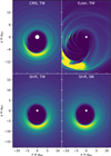 |
Fig. 6 Snapshot of the surface densities of the high resolution simulations with a binary eccentricity of 0.4. We plot the simulation using the Euler indirect at a simulation time of t = 800 Tbin, and the other simulations at t = 4000 Tbin. All plots use the same linear color scale. |
5 Protoplanetary disk with hot Jupiter
In this section, we test whether our proposed changes are relevant to more common scenarios of planet-disk interactions. We used a setup of a central star of mass mstar = 1 M⊙ and a companion object with masses of m = [1,3,10,50] MJup (corresponding to mass ratios of q ≈ 0.1%, 0.3%, 1%,5%) on a circular orbit (e = 0) with an initial semi-major axis of 1 au. At the beginning of the simulation, the companion was on a fixed orbit and was treated as massless when interacting with the disk. The mass of the companion felt by the gas was then ramped up over the first 50 orbital periods according to
![Mathematical equation: $m(t) = \left\{ {\matrix{ {m \cdot \left[ {1.0 - {{\cos }^2}\left( {t \cdot 2\pi /50{T_{{\rm{orb }}}}} \right)} \right],} \hfill & {t < 50{T_{{\rm{orb }}}}} \hfill \cr{m,} \hfill & {t \ge 50{T_{{\rm{orb }}}}.} \hfill \cr } } \right.$](/articles/aa/full_html/2025/01/aa50383-24/aa50383-24-eq26.png) (14)
(14)
Despite the mass ramping, the gas velocities were always initialized in the center-of-mass frame of the N-body system with their fully ramped-up masses.
The gravitational potential of the N-body system at the position of a cell was computed as a Plummer potential with a smoothing length of ϵ = 0.6H (Müller et al. 2012), where H = h ⋅ r is the gas scale height. The potential reads:
 (15)
(15)
where G is the gravitational constant,  , is the smoothed distance between the gas cell i and the N-body object k with mass Mk. Similarly, the force exerted by the gas on the N-body objects was calculated as
 (16)
(16)
where mi is the mass of the gas cell and fsm is the smoothing function by Crida et al. (2009):
![Mathematical equation: ${f_{{\rm{sm}}}}(s) = {\left[ {\exp \left( { - 10\left( {{s \over {0.8{r_H}}} - 1} \right)} \right) + 1} \right]^{ - 1}},$](/articles/aa/full_html/2025/01/aa50383-24/aa50383-24-eq30.png) (17)
(17)
where rH is the Hill radius according to Eggleton (1983). The smoothing was applied only to the companion object, not to the star. It acts as a filter to remove the effects of a disk around the companion, since the disk is poorly resolved and not realistically modeled in our setup.
The disk was locally isothermal (α = 10−3, h = 0.05). The simulation domain ranges from 0.25 au to 25 au and the cells are spaced logarithmically in the radial direction and uniformly in the azimuthal direction with a resolution of Nr × Nφ = 739 × 1005, which corresponds to eight cells per scale height. The surface density was initialized as
![Mathematical equation: $\Sigma (d) = 200{\rm{g}}{\rm{c}}{{\rm{m}}^{ - 2}} \cdot {(d/1{\rm{au}})^{ - 0.5}} \cdot {1 \over {1 + \exp [(d - 12{\rm{au}})/0.25{\rm{au}}]}},$](/articles/aa/full_html/2025/01/aa50383-24/aa50383-24-eq31.png) (18)
(18)
where d is the distance to the center-of-mass of the N-body system. We applied strict outflow boundary conditions at the inner and outer boundaries. Since the location of the boundaries depends on the frame of reference, we added an exponential cutoff at 12 au to prevent the disk from interacting with the outer boundary instead of applying damping conditions in the outer regions. We measured the accretion on the companion using the accretion model of Kley (1999), that is, we removed a fraction of the gas from the Hill sphere of the companion at each time step with a half-emptying time of 1000 Torb. The mass of the gas and its momentum were added to the companion.
The first 200 orbital periods were used for initialization, during which time the disk exerted no force on the star or companion, and gas accretion by the companion was not active. Then disk feedback and companion accretion were activated, and the simulations were run for another 1800 orbital periods. The companion then migrated under the gravitational influence of the disk and due to momentum accretion. The gravitational force of the gas on the star was added to the indirect term of the simulation. The N-body system was always shifted to the frame of the star at the end of each time step.
The way the disk is initialized can affect the long-term evolution of the disk. In our previous runs, the simulations centered on the star were also initialized around the star so that the surface density was a function of the distance of the cell from the star, and the initial gas velocity was computed with the mass of the star. This caused the disk to become eccentric for high companion masses (m ⪆ 10 MJup) as the companion ramped up in mass. An example of this is shown in the third row of Fig. 8. For m = 10 MJup (left side) these effects start to become noticeable, while for m = 50 MJup (right side) the entire disk and the gap around the companion become eccentric. This does not happen if the disk is initialized using the distance to the center of mass and the total mass of the N-body system to compute the velocities, as demonstrated for simulations centered on the star (second row) and centered on the center of mass (first row).
For even more massive stellar-mass companions, it is no longer possible to ramp up the mass of the companion, because the missing gravity from the not yet fully ramped up companion would cause the disk to deform before the companion reaches its final mass. Without ramping, longer initialization times are required because strong shocks occur during the clearing of the gap that depend on the artificial viscosity. These initialization artifacts then resolve on viscous time scales.
The advantage of centering the disk on the primary instead of the center of mass is also demonstrated in Fig. 8. At high masses (top-right panel), the primary orbits inside the inner radius, causing its stellar disk to quickly accrete through the inner boundary. This does not happen when the simulation is centered on the primary (middle-right panel), in which case the disk is optimally resolved by the grid, which is the main motivation for this study.
After an initialization phase of 200 companion orbits, we enabled the interaction between the disk and the companion and continued the simulations, meaning that the companion migrates under the gravitational influence of the disk, while the gravity of the gas on the star was added to the indirect term of the simulation. With feedback enabled, the forces exerted on the binary system can move its center of mass, so we shifted the N-body system to the new center of mass of the binary after each time step. This was not necessary during the initialization phase because the forces were turned off and the center of mass of the binary stayed put.
We then monitored the mass accretion rate on the companion, the torque exerted by the gas on the companion, the eccentricity and the semi-major axis of the companion. The results for a m = 1 MJup companion are shown in Fig. 9. We find no significant differences between the different artificial viscosities, indirect term protocols, or coordinate centers. The gas torques oscillate for a longer time in the SN artificial viscosity simulations, but they settle to the same value as in the TW artificial viscosity simulations and from then on evolve the same. Although the eccentricity variations display factor of 2 difference between the runs, the overall level of planetary eccentricity is too small (~ 10−3) to be considered a significant effect, and the differences do not appear to be related to the artificial viscosity or the indirect term protocol.
For higher masses of m = 3 MJup and m = 10 MJup, we find small differences within the Hill sphere of the companion that we can directly attribute to the different artificial viscosity prescriptions (cf. Fig. A.2). Globally, we find that the time at which the gap becomes eccentric is different for each setup. When the gap becomes eccentric, the density inside the gap is higher, leading to higher accretion (see first panel in Fig. 10) and the gas torque changes (see second panel). The differences in gas torque then lead to different eccentricities and migration rates of the companion. Most of the differences between the setups can be explained by the different time at which the gap becomes eccentric. We find found no trend in how the artificial viscosity or the indirect term protocol affects the timing of this transition. While the simulations are in the same state, they evolve similarly.
For our high-mass companions (m = 30 MJup and m = 50 MJup), we find significant differences in mass accretion between the artificial viscosities, as shown in Fig. 11. The artificial viscosities eject mass from the Hill sphere of the companion (cf. Fig. A.3) resulting in lower mass accretion rates. As depicted in the first panel of Fig. 11, we find ≈50% higher accretion rates and ≈50% more mass inside the Hill sphere for the TW artificial viscosity. This difference increases to almost 100% for the m = 50 MJup companion.
Because we have ignored the gravitational effect of the gas inside its Hill sphere on the companion by Eq. (17), the differences in gas torque are an indication of the effects of the different setups far away from the companion. Again, we find that there are differences in gas torque and companion eccentricity between the setups, but without a clear trend. This means that there is no strict increase or decrease in gas torque or eccentricity when changing the artificial viscosity or the indirect term prescription.
However, in most of our simulations, we find that the companion migrates inwards faster for the TW artificial viscosity. For example, in the last panel of Fig. 11, we find 7% faster inward migration for the TW artificial viscosity than the SN artificial viscosity in the primary frame and 5% faster in the center-of-mass frame. We analyzed what causes this difference and found that in the center-of-mass frame, the gas torque on the planet is stronger for the TW artificial viscosity; and in the primary frame, the indirect term due to the gas feedback on the central star, which results in a positive torque on the companion, is weaker for the TW artificial viscosity. At the end of the simulations (t = 1800 Torb to 2000 Torb), the migration rates are similar for all setups. It remains to be determined whether the faster inward migration observed with the TW artificial viscosity represents a consistent trend or a coincidental effect.
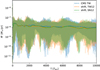 |
Fig. 7 Mass accretion rate of the circumbinary disk through the inner boundary over time. The dashed lines show the moving average over 100 binary orbits. |
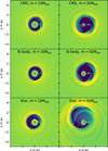 |
Fig. 8 Snapshot of the logarithm of the surface density of a mass-less disk at the end of the initialization period (t = 200 Porb). “CMS” indicates that the simulation is in the center-of-mass system, and “star” indicates that the simulation is centered on the star and the disk has been initialized around the star. “N-body” indicates that the simulation is centered on the star, but the disk has been initialized around the center of mass of the N-body system. All plots use the same color scale. |
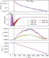 |
Fig. 9 Various quantities measured for a m = 1 MJup companion. Plotted are the mass accretion rate by the companion, the gas torques exerted by the disk on the companion, the eccentricity, and the normalized semi-major axis of the companion. |
6 Summary and conclusions
We have presented two modifications to the FARGO code (Masset 2000) that allow us to simulate a circumbinary disk in the frame of one of the stars, which to our knowledge was not possible before. One of the proposed modifications is the use of the tensor artificial viscosity by Tscharnuter & Winkler (1979) and the other is a new method for calculating the indirect term. We have also tested their relevance to simulations of planet-disk interactions.
First, we studied the indirect term prescription, that is, the consideration of fictitious forces due to a non-inertial frame of reference. In Sect. 2, we noted that the standard method of applying the indirect term is comparable to a forward Euler step and produces results comparable to that of a Euler integrator. It fails to keep the central object at the coordinate center and similarly fails to keep other objects in the frame of the central object. We proposed to precompute the effective acceleration experienced by the central object over the entire time step and use it as the indirect term. This method is comparable to advancing the whole system in time and then subtracting the velocity of the central object at the end of the time step. This shift-based indirect term will by design keep the velocity of the central object at the end of the time step at 0. We then showed that at large radii, r > 2 abin, it is significantly better at modeling the effects on a non-inertial frame of reference than the default method.
The proposed shift-based indirect term protocol should also be applicable to other grid codes used to simulate the interaction of disks with stars and planets. For example, the PLUTO code has a hydrodynamics solver that uses a higher-order time-stepping scheme, but in the versions known to the authors, the synchronization between the hydrodynamics and N-body solvers is performed once per integration time step and the indirect term is applied as a single Euler step. We expect that synchronization at each substep would improve the accuracy of the evolution of the combined N-body and hydrodynamics system. How this plays out in practice remains to be seen.
In Sect. 3 we listed literature (Tscharnuter & Winkler 1979; Stone & Norman 1992; Bodenheimer et al. 2006), which already noted that the artificial viscosity by Von Neumann & Richtmyer (1950), which is the default artificial viscosity in the FARGO (Masset 2000) and FARGO3D codes (Benítez-Llambay & Masset 2016), is not suitable for curvilinear coordinates and can cause artificial pressure for smooth gas flows even in the absence of shocks. They also stated that the tensor artificial viscosity by TW79 should be preferred because it takes into account the geometry of the grid and is independent of the frame of reference. We confirmed these claims and showed that the artificial viscosity by VNR50 inherently produces an artificial pressure in a smooth Keplerian disk that arises from the velocity gradients in the non-inertial frame of reference and scales with the number of azimuthal cells as  .
.
In Sect. 4, we simulated a circumbinary disk in the center of the lower-mass companion of a binary system. In this setup, the indirect forces reach magnitudes several times stronger than the direct gravitational forces of the N-body system, and the standard indirect term prescription causes the disk to disperse. Our shift-based indirect term prescription keeps the disk stable, even at low resolutions, and allows the simulations to converge to a reference simulation in the center-of-mass frame with increasing spatial and temporal resolution.
At low resolutions, the artificial pressure generated by the VNR50 artificial viscosity caused by the velocity gradients in the non-inertial frame of reference, was strong enough to prevent the disk from precessing, leading to significant eccentricity growth in the disk. At high resolutions (>8 cells per scale height) the simulation starts to converge for the different artificial viscosities.
We then tested the relevance of our changes to planet-disk interaction simulations in Sect. 5. At low companion masses of m ≤ 1 MJup, we find no differences between the artificial viscosities or the indirect term protocols. The default methods in the original FARGO code (Masset 2000) are sufficient for these simulations.
For companion masses m ≥ 3 MJup it becomes relevant to initialize the disk in the center-of-mass frame instead of the center of the star. Otherwise, the shift of the center of mass caused by the ramping of the companion mass can cause the disk to become eccentric. In addition, the artificial viscosity by VNR50 produces artificial pressure inside the Hill sphere of the companion (see also Appendix A).
For even higher masses, m ≥ 30 MJup, it does become necessary to initialize the disk in the center-of-mass frame or the disk will become unstable as the companion mass ramps up. In addition, the artificial viscosity VNR50 ejects significant amounts of mass from the Hill sphere of the companion, resulting in lower mass accretion rates. We also found differences in the gas feedback from the companion depending on the choice of artificial viscosity and indirect term protocol, but these differences are small.
In summary, we find that the methods used in the FARGO code (Masset 2000) are sufficient for simulating planet-disk interactions in the frame of a central star, but issues arise for more massive companion objects. When the companion mass approaches the brown dwarf mass, the frame in which the disk is initialized has to be adjusted, and the artificial viscosity by Von Neumann & Richtmyer (1950) will cause artificial mass ejection from the Hill sphere of the companion. Initializing the disk in the center-of-mass frame would also be relevant for any other grid code centered on the star.
For stellar mass companions, the artificial acceleration caused by the Von Neumann & Richtmyer (1950) artificial viscosity due to the indirect term can cause eccentricity growth throughout the disk. Problems related to artificial viscosity can be mitigated by using the tensor artificial viscosity by Tscharnuter & Winkler (1979). In addition, for stellar mass companions, the indirect term becomes several times stronger than the direct gravitational forces of the N-body system inside the circumbinary disk. In such cases, more accurate indirect-term prescriptions should be used. We believe that the shift-based indirect term protocol presented in this work is a good choice when the indirect term is applied in a single step per time step.
Acknowledgements
TR acknowledges funding from the Deutsche Forschungs-gemeinschaft (DFG) research group FOR 2634 “Planet Formation Witnesses and Probes: Transition Disks” under grants KL 650/29-2. The authors acknowledge support by the High Performance and Cloud Computing Group at the Zentrum für Datenverarbeitung of the University of Tübingen, the state of Baden-Württemberg through bwHPC and the German Research Foundation (DFG) through grant INST 37/935-z1 FUGG.
Appendix A Companion disk
In Sect. 5 we measured the effects of the artificial viscosities far from the companion by excluding the torques inside the Hill sphere. While the accretion rate depends on the amount of mass inside the Hill sphere, it is unclear how much it is affected by the different migration rates.
In this section, we isolate the effects of the artificial viscosities inside the Hill sphere of the companion. To achieve this, we ran simulations with the same parameters as in Sect. 5, but kept the central star and companion on fixed orbits by disabling disk feedback. Additionally, we tried to remove the circumstel-lar disk by reducing the domain size to 0.6 au to 1.5 au with a resolution of Nr × Nφ = 147 × 1005 (cell sizes remained the same). Removing the circumstellar disk from the simulation isolates the gap region, and thus, we are able to avoid contributions to the mass of the Hill sphere that would otherwise stem from gas traversing the gap. As before, we used strict outflow conditions at both boundaries. To reach a steady state, we kept the mass inside the simulation domain constant by rescaling the surface density of each cell after each time step by a factor equal to the initial gas mass divided by the current gas mass. This density rescaling function adds the outflowing mass preferentially to cells with high density. Since gas feedback is not considered here, the surface density cancels out in the momentum equations and the actual disk mass is not relevant.
The surface density profiles after 200 orbital periods are shown in Fig. A.1 for different companion masses, m. In principle, the 3MJup planet in the upper plot clears its orbit, but because the mass is replenished by the density rescaling function, the gap region appears to be filled with gas. What the plot actually shows is the density ratio between the gap region and the circumplane-tary disk. While this setup is not physical, it allows us to compare the effects of the different numerical methods by measuring the amount of mass held inside the Hill sphere of the companion.
The normalized amount of mass inside the Hill sphere over time is shown in Fig. A.2 for the m = 3MJup companion. Neither the frame of reference nor the indirect term prescription affects the amount of mass around the companion, but for the artificial viscosities, differences become visible after 100 Porb. At the end of the simulation, the Hill sphere contains 8% more mass for the SN artificial viscosity. We repeated this test for a m = 1MJup companion, and found a difference of only 0.3% in mass inside the Hill sphere. Similar to the long range effects probed in Sect. 5, we again find that the choice of artificial viscosity will affect the simulations at these companion masses.
For companion masses m = 10MJup and above, the companion clears its orbit and almost all of the gas mass accumulates inside the Hill sphere (see the lower plot in Fig. A.1). Since the mass inside the Hill sphere is the same for all setups, we measure the effect of the artificial viscosities by how much mass is ejected from the companion disk through the inner and outer boundaries of the domain.
The two lower panels in Fig. A.3 show the mass loss rates for the different setups with a m = 50MJup companion. The effects of the indirect term protocol are still negligible. The artificial viscosity again has the largest effect with the SN artificial viscosity leading to 10 times more mass ejection than the TW artificial viscosity in the CMS and 5 times more in the primary frame simulations. At this mass, the frame of reference also makes a difference with the primary frame simulations ejecting 3 and 1.5 times more mass than the CMS simulations for the TW and SN artificial viscosities, respectively. Without the mass replenishment function, the companion disks would lose mass, leaving less mass for accretion and explaining the different mass accretion rates found in Fig. 11.
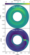 |
Fig. A.1 Surface densities after 200 orbital periods for different companion masses. The dashed cyan line represents the Roche lobe of the system. Both simulations were run in the center-of-mass frame and used the TW artificial viscosity. Both plots use the same color scale. |
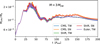 |
Fig. A.2 Disk inside the Hill sphere of a m = 3 MJup companion divided by the total gas mass inside the simulation domain for different simulation setups. |
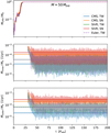 |
Fig. A.3 Disk mass and mass loss rates over time for a m = 50 MJup companion for different setups. Top panel: Mass inside the Hill sphere of the companion. Second panel: Mass loss rate through the inner boundary. Bottom panel: Mass loss rate through the outer boundary. All quantities are normalized to the total gas mass inside the domain. |
For the m = 10MJup the mass loss is higher for the TW artificial viscosity by a factor of 12% and 100% for the inner and outer boundary respectively, which is similar to the higher disk masses measured for the m = 3MJup companion in Fig. A.2. This implies that between 10 and 30 Jupiter masses, the SN artificial viscosity becomes more active and changes from lower to higher mass ejection than the TW artificial viscosity.
References
- Benítez-Llambay, P., & Masset, F. S. 2016, ApJS, 223, 11 [Google Scholar]
- Bodenheimer, P., Laughlin, G. P., Rozyczka, M., et al. 2006, Numerical Methods in Astrophysics: An Introduction. Series in Astronomy and Astrophysics (Taylor & Francis) [Google Scholar]
- Crida, A., Baruteau, C., Kley, W., & Masset, F. 2009, A&A, 502, 679 [NASA ADS] [CrossRef] [EDP Sciences] [Google Scholar]
- Duffell, P. C., Dittmann, A. J., D’Orazio, D. J., et al. 2024, ApJ, 970, 156 [NASA ADS] [CrossRef] [Google Scholar]
- Eggleton, P. P. 1983, ApJ, 268, 368 [Google Scholar]
- Klahr, H., & Kley, W. 2006, A&A, 445, 747 [NASA ADS] [CrossRef] [EDP Sciences] [Google Scholar]
- Kley, K. 1999, MNRAS, 303, 696 [NASA ADS] [CrossRef] [Google Scholar]
- Masset, F. 2000, A&AS, 141, 165 [NASA ADS] [CrossRef] [EDP Sciences] [Google Scholar]
- Müller, T. W. A., Kley, W., & Meru, F. 2012, A&A, 541, A123 [NASA ADS] [CrossRef] [EDP Sciences] [Google Scholar]
- Rein, H., & Liu, S. F. 2012, A&A, 537, A128 [NASA ADS] [CrossRef] [EDP Sciences] [Google Scholar]
- Rein, H., & Spiegel, D. S. 2015, MNRAS, 446, 1424 [Google Scholar]
- Rometsch, T., Jordan, L. M., Moldenhauer, T. W., et al. 2024, A&A, 684, A192 [NASA ADS] [CrossRef] [EDP Sciences] [Google Scholar]
- Shakura, N. I., & Sunyaev, R. A. 1973, A&A, 500, 33 [NASA ADS] [Google Scholar]
- Stone, J. M., & Norman, M. L. 1992, ApJS, 80, 753 [Google Scholar]
- Thun, D., Kley, W., & Picogna, G. 2017, A&A, 604, A102 [NASA ADS] [CrossRef] [EDP Sciences] [Google Scholar]
- Tscharnuter, W. M., & Winkler, K. H. A. 1979, Comput. Phys. Commun., 18, 171 [NASA ADS] [CrossRef] [Google Scholar]
- Von Neumann, J., & Richtmyer, R. D. 1950, J. Appl. Phys., 21, 232 [NASA ADS] [CrossRef] [Google Scholar]
All Tables
All Figures
|
Fig. 1 Time evolution over three binary periods of the primary under the influence of the indirect term protocols of Eqs. (1) and (2). |
| In the text | |
|
Fig. 2 Time evolution of the semi-major axis and eccentricity of two test particles under the influence of the indirect term in Eq. (1) and Eq. (2) respectively and an exact reference case without an indirect term. |
| In the text | |
|
Fig. 3 Amplitudes of the semi-major axis oscillations as a function of the initial semi-major axis. The dotted line at 3 abin indicates the initial position of the particle that is used for the time step criteria. The dashed lines represent the best least squares fit with a power law model. |
| In the text | |
|
Fig. 4 Snapshot of the azimuthal velocity (left) and artificial acceleration due to Eq. (13) in the frame of the secondary (right). The red dot represents the secondary, the green dot represents the primary, and the black dashed line represents the orbit of the primary. The arrows indicate the direction of motion and are not to scale. The binary and grid parameters are the same as in Sect. 4. |
| In the text | |
|
Fig. 5 Snapshot of the surface density after 5000 binary orbits of a massless disk around a binary system with qbin = 0.5 and ebin = 0.4. The plots show the results for different combinations of coordinate centers, artificial viscosity, and indirect term protocol. All plots use the same linear color scale. |
| In the text | |
|
Fig. 6 Snapshot of the surface densities of the high resolution simulations with a binary eccentricity of 0.4. We plot the simulation using the Euler indirect at a simulation time of t = 800 Tbin, and the other simulations at t = 4000 Tbin. All plots use the same linear color scale. |
| In the text | |
|
Fig. 7 Mass accretion rate of the circumbinary disk through the inner boundary over time. The dashed lines show the moving average over 100 binary orbits. |
| In the text | |
|
Fig. 8 Snapshot of the logarithm of the surface density of a mass-less disk at the end of the initialization period (t = 200 Porb). “CMS” indicates that the simulation is in the center-of-mass system, and “star” indicates that the simulation is centered on the star and the disk has been initialized around the star. “N-body” indicates that the simulation is centered on the star, but the disk has been initialized around the center of mass of the N-body system. All plots use the same color scale. |
| In the text | |
|
Fig. 9 Various quantities measured for a m = 1 MJup companion. Plotted are the mass accretion rate by the companion, the gas torques exerted by the disk on the companion, the eccentricity, and the normalized semi-major axis of the companion. |
| In the text | |
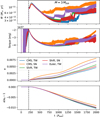 |
Fig. 10 Same as Fig. 9 but for a m = 3 MJup companion. |
| In the text | |
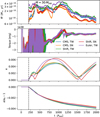 |
Fig. 11 Same as Fig. 9 but for a m = 30 MJup companion. |
| In the text | |
|
Fig. A.1 Surface densities after 200 orbital periods for different companion masses. The dashed cyan line represents the Roche lobe of the system. Both simulations were run in the center-of-mass frame and used the TW artificial viscosity. Both plots use the same color scale. |
| In the text | |
|
Fig. A.2 Disk inside the Hill sphere of a m = 3 MJup companion divided by the total gas mass inside the simulation domain for different simulation setups. |
| In the text | |
|
Fig. A.3 Disk mass and mass loss rates over time for a m = 50 MJup companion for different setups. Top panel: Mass inside the Hill sphere of the companion. Second panel: Mass loss rate through the inner boundary. Bottom panel: Mass loss rate through the outer boundary. All quantities are normalized to the total gas mass inside the domain. |
| In the text | |
Current usage metrics show cumulative count of Article Views (full-text article views including HTML views, PDF and ePub downloads, according to the available data) and Abstracts Views on Vision4Press platform.
Data correspond to usage on the plateform after 2015. The current usage metrics is available 48-96 hours after online publication and is updated daily on week days.
Initial download of the metrics may take a while.