| Issue |
A&A
Volume 693, January 2025
|
|
|---|---|---|
| Article Number | A103 | |
| Number of page(s) | 14 | |
| Section | Stellar structure and evolution | |
| DOI | https://doi.org/10.1051/0004-6361/202450333 | |
| Published online | 07 January 2025 | |
A Maia-type candidate was misclassified: V424 Cep is an eclipsing β Cep-type pulsator in a triple system⋆
1
Physikalisch-Meteorologisches Observatorium Davos and World Radiation Center, Dorfstrasse 33, CH-7260 Davos Dorf, Switzerland
2
Instituto de Ciencias Físicas, Universidad Nacional Autónoma de México, Ave. Universidad S/N, Chamilpa, Cuernavaca, Mexico
3
Indiana University, 107 S. Indiana Avenue, Bloomington IN 47405-7000, USA
4
Weierstrasse 30, CH-8630 Rueti, Switzerland
5
Observatorio Astronómico Nacional, Instituto de Astronomía, Universidad Nacional Autónoma de México, Ensenada, B.C., Mexico
⋆⋆ Corresponding author; This email address is being protected from spambots. You need JavaScript enabled to view it.
Received:
11
April
2024
Accepted:
10
November
2024
Abstract
Context. V424 Cephei is an eclipsing binary system that has been classified as a Maia variable candidate. These objects are pulsators that apparently lie outside the theoretical instability strips.
Aims. We determine the properties of V424 Cep and identify the nature of the pulsating variable.
Methods. We analyzed photometric data obtained over the past three decades from TESS, Gaia, Hipparcos, and ground-based observations. Times of minimum light were determined, and the light curves and spectral energy distribution were analyzed. We analyzed the radial velocity curves of the double-lined system obtained from spectroscopy at the Observatorio Astronómico Nacional on the Sierra San Pedro Mártir.
Results. The two eclipses observed in the light curves yield a refined orbital period P = 4.93 d, an eccentricity e = 0.02, and an apsidal period U = 730 yr. The eclipse O–C curve is not linear. Combined with the apsidal period, this indicates the presence of a third component in the system. This conclusion was confirmed by a comparison of predicted and observed absolute fluxes. The masses of the binary pair are 8.7 M⊙ and 6.3 M⊙, their radii are 6.0 R⊙ and 3.5 R⊙, and the luminosities are log(L/L⊙) 3.80 and 3.11. The TESS light curve shows oscillations with a dominant period of 0.17 d. They are coherent throughout the orbital cycles with a stable amplitude, except during the (partial) eclipse of the primary star. This indicates that this is the pulsator. Its temperature is 21 000 K. The third-light component contributes no more than 15% to the total light of the system in the TESS wavelength band and 20% in the K band.
Conclusions. V424 Cep is not a Maia variable, but rather a β Cep star. This result highlights the importance of combining photometric light-curve solutions with absolute flux models and spectroscopic observations.
Key words: asteroseismology / eclipses / binaries: eclipsing / stars: oscillations / stars: individual: V424 Cep / stars: individual: HD 239652
Based in part on observations carried out at the Observatorio Astronómico Nacional on the Sierra San Pedro Mártir (OAN-SPM), Baja California, México.
© The Authors 2025
 Open Access article, published by EDP Sciences, under the terms of the Creative Commons Attribution License (https://creativecommons.org/licenses/by/4.0), which permits unrestricted use, distribution, and reproduction in any medium, provided the original work is properly cited.
This article is published in open access under the Subscribe to Open model. This email address is being protected from spambots. You need JavaScript enabled to view it. to support open access publication.
1. Introduction
Pulsating stars in eclipsing binary systems are crucial for testing stellar structure and evolution theories. Their radii, masses, and surface equatorial rotation velocity can be directly determined from observations, which constrains these important parameters. Their pulsation frequencies can be compared to those predicted from asteroseismology, and this provides constraints on the conditions of the stellar interior properties such as opacity, convection, and rotation structure (see Aerts 2021 and Kurtz 2022 for reviews of these topics).
The Hertzsprung-Russel diagram (HRD) contains several classes of pulsating stars that lie along the theoretical pulsational instability strip (Dupret et al. 2004; Szewczuk & Daszyńska-Daszkiewicz 2017). They are classified as γ Dor, δ Sct, slowly pulsating B-stars (SPBs) and β Cep. The mass range in which each of these prevails is smallest in the first and largest in the last objects (see Fig. 1 in Kurtz 2022). There is a gap between the δ Sct and SPBs in which no pulsationally unstable stars are predicted in standard stellar models. However, Mowlavi et al. (2013) found a group of variable stars in NGC 3766 that are located in the HRD between the red edge of the SPBs and the blue edge of the δ Sct stars. Their pulsation periods were found to be in the range from 0.1 to 0.7 d, with amplitudes between 1 and 4 mmag. In recent years, the Maia-type class of variables was added to the list of pulsating objects. Their properties are not predicted by theory. These variables are located in the main-sequence region, which corresponds to stars with 3–7 M⊙, which are cooler than the β Cepheid variables and hotter than the δ Scuti variables. This overlaps with the SPB region, but the pulsation periods of the Maia stars are shorter than those of SPBs, and they are not predicted by stability analyses. Balona & Ozuyar (2020) defined a limiting period 0.2 d that separates SPBs from the Maia variables (see their Fig. 2), whose limiting period is ≈0.25 d (Aerts 2021). Balona et al. (2016) also noted that Maia variables have multiple high frequencies, indicating that these are p modes and not g modes, as for SPBs.
The existence of a Maia class of variables has recently been questioned by Kahraman Aliçavuş et al. (2024), who argued that most stars that were proposed to be pulsators outside the well-established instability domains are most likely misclassified.
V424 Cep is also known as HD 239652 or Hip 105690. It is an eclipsing binary (P = 4.9 d) discovered by Hipparcos, and (Kazarovets et al. 1999) assigned its General Catalogue of Variable Stars designation. Chen et al. (2022) noted pulsations in its light curve and classified the star as a Maia candidate on the basis of its Gaia temperature.
It is a program star of a project that recorded the times of observed light minima and compared them with the times predicted from the binary ephemerides. The observed minus computed data were published at the O−C gateway (Paschke & Brat 2006). While complementing minima timings for this system, we observed its striking pulsations with a period ≈0.17 d. This period is slightly shorter than the limit of 0.2 d quoted above that is present in the SPBs, but it is within the range of the β Cepheid-type pulsators (Stankov & Handler 2005; Shi et al. 2024).
V424 Cep was assigned an approximate spectral type of B5 by Cannon & Pickering (1993), implying a temperature for the brighter component in the range of 15 000 K. However, the quality indication for this temperature determination was cited as E, which corresponds to the poorest quality. Hence, this temperature value is quite uncertain. From spectra obtained for measuring B star radial velocities Petrie & Pearce (1961) determined a spectral type of B4, which implies a temperature of about 16 400 K. The stellar properties deduced from Gaia DR3 photometry are Teff = 17 070 ± 90 K, logL/L⊙ = 3.7 ± 0.02, and logg = 3.46 ± 0.01 (Gaia Collaboration 2016, 2023a,b). The Gaia temperature implies a spectral type B3, which is below the lower limit for the β Cepheid variables. This lower limit is about at 18 000 K. It is important to note, however, that this temperature estimate does not account for the binary nature of the system, which raises the question as to whether a higher value might be possible. This would make the primary star a β Cep and would eliminate the difference between the properties determined thus far and the theory of stellar pulsations.
The assumption that the magnitude and colors of V424 Cep can be used to deduce its effective temperature is limited because it neglects the presence of the close companion. It also neglects the possible presence of a third component in the system, which we show in this paper is indeed present.
In Sect. 2 we describe the photometric data and their measurements, which are analyzed for apsidal motion and a light time effect in Sect. 4. This leads to the conclusion that there is a third object in the system. Section 3 describes the spectroscopic observations. The pulsation periods are determined in Sect. 5 and are shown to arise in the primary (brighter) member of the eclipsing pair. In Sect. 6 we analyze the light curve and spectral energy distribution. We constrain the contribution of the third source and illustrate the uncertainties on the stellar properties when they are derived without radial velocity information. In Sects. 7 and 8 we present a discussion and the conclusions.
2. Photometric measurements
2.1. TESS observations
V424 Cep (also known as TIC 315777423) was observed by the TESS satellite (Ricker et al. 2015) in sectors 15, 16, 17, 56, 57, 76, and 77, each sector having a duration of approximately 26 d. It is a target for the so-called postage-stamp-type of monitoring with an observational cadence of 2 min, except for sector 16, for which observations were obtained with a 30 min interval. The data files were downloaded from the Mikulski Archive for Space Telescopes (Swade et al. 2019) using search_lightcurve (Ginsburg et al. 2019). These files contain fluxes, termed SAP_FLUX, as reduced by the TESS pipeline. The light curves are the result of aperture photometry, which gives total counts measured within the photometric aperture from the TESS images.
The light curves were extracted and normalized with the software provided by the Lightkurve Collaboration (2018). In sector 16, the flux increases toward the data gaps at perigeum of the satellite orbit. Inspection of the background fluxes reveals that this is due to strongly increased straylight, and we masked the intervals of increased fluxes out.
The top panel of Fig. 1 displays the data sets of sectors 15 (blue), 16 (orange), and 17 (green) in full time resolution. The lower panel of this figure zooms into a fragment of 6 days that we extracted from sector 56. The flux scale was chosen to clearly show the 0.17 d pulsations.
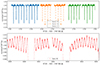 |
Fig. 1. Light curves of V424 Cep observed by the TESS satellite. Top: 79 d of the observations in sectors 15–17 (August 15, 2019, to October 7, 2019). Bottom: 6 d extract from the sector 56 observations (September 2022) plotted with the full time resolution of 2 min. The symbol size shows the precision of the individual measurements. The vertical scale is chosen to illustrate the pulsations, and it therefore truncates the eclipses. |
The light curve illustrated in Fig. 1 shows primary minima with a depth of about 76% of the light, that is, a flux reduction of 0.30 mag, and secondary minima with a depth of 81% (0.23 mag). The epochs of minima in the light curve of V424 Cep were measured with two methods. The first method was the optimize routine from the Python SciPy package (Virtanen et al. 2020), which fit a Gauss-like function aexp(−(∣(t−T0)∣/Δt)γ) to each normalized eclipse curve, yielding the epoch of minimum, T0. The free parameters Δt, a, and γ describe the duration and shape of the eclipse curve. The second method was the algorithm proposed by Kwee & van Woerden (1956, hereafter the KvW method). The two methods yield very similar but not identical results. On average, the difference in the minimum epochs determined by the two methods is 12 ± 9 s, except for sector 16, which has measurements with 30 min intervals, for which the differences are some minutes. The average uncertainty determined by the Gauss-fit method is 20 s, the uncertainty from the KvW method is 15 s, and it is some minutes for sector 16.
The uncertainties of the measured minimum epochs can be verified because the minimum timings of each eclipse type have to lie on a linear ephemeris at least for time intervals that are shorter than any plausible apsidal motion or light travel-time timescales (see Sect. 4). The deviations from a linear fit reveal that the statistical uncertainties are 60 s and 90 s for the primary minimum and secondary minimum, respectively. Thus, empirically, that is, assuming that a linear ephemeris is valid, the uncertainties of the minima are considerably larger than the precision given by the methods. As the pulsations (see Fig. 1 and Sect. 5) may have a systematic influence, we removed the 20 strongest periods in the 40 to 200 μHz range form the combined light curve. This indeed improved the fits to the minima, such that the average uncertainty determined by the Gauss-fit method decreased to 12 s and the uncertainty of the KvW method to 8 s for the 2 min sampled data. The statistical deviation from averages of the values in the three TESS observation intervals, that is, sectors 15–17, 56–57, and 76–77, also decreased, to 40 s, but the uncertainties derived from the empirical statistics remained larger by about a factor of four than the uncertainty estimates by the methods.
We list in Tables A.1 and A.2 the minimum epochs resulting from the Gauss-fit method, but we multiply their uncertainties by a factor of four in order to reflect the empirically determined uncertainties. The minima of TESS sectors 15 and 17 have been reported in Paschke (2023). The values in Table A.1 differ by a few seconds from the previously reported ones because the new minima were calculated from fits to a light curve without pulsations.
At the beginning of the TESS data set in 2019, the secondary minimum occurred ΔT = 2.47761 ± 0.0004 d after the primary minimum. If the orbit were circular, secondary eclipses should occur a time P/2 after the time of primary eclipse, where P is the orbital period in Eq. (1). However, ΔT differs from P/2 by 0.012 d. This difference indicates that the orbit is eccentric.
The average of the separation in time between each successive primary eclipse yields an average period for the primary minima and similarly for the secondary eclipses. We find that the average period of secondary eclipses differs from that of the primary eclipses by 0.7 s. This difference is the signature of apsidal motion, which we discuss below. We determined a preliminary orbital period by taking the average of these two periods and define an ephemeris as follows:
 (1)
(1)
where E is a whole number corresponding to the orbital cycle, starting with an initial epoch as defined by the first minimum in sector 15 (see Fig. 1). The period P is the average of the periods determined separately from the primary and secondary minima. We do not quote uncertainties for this equation because it only gives a preliminary ephemeris that is valid for the TESS data set described in this section. Prša et al. (2022) derived an ephemeris from observations of TESS sectors 15 to 17, which agrees within their uncertainties with Eq. (1).
The values of the differences in the observed to computed minima using the above reference ephemeris are plotted in Fig. 2. The primary and secondary values of O−C are plotted separately, and we introduced a constant shift of −17 min (= − 0.012 d) to those of the secondary to facilitate the comparison with those of the primary. The three panels of this figure correspond to 2019 (sectors 15–17), 2022 (sectors 56–57), and 2024 (sectors 76–77) and clearly show that the average O−C values of each of the primary and secondary minima are similarly displaced from one panel to the next. These offsets are the signature of either a changing apsidal period or a light time effect. We analyze these possibilities below.
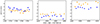 |
Fig. 2. Observed minus computed epochs of primary minima (blue) and secondary minima (orange) using the reference ephemeris of Eq. (1). The mean deviation of the secondary minima from Eq. (1), which is <O−C>2 = 17 min, was subtracted to facilitate the comparison of its behavior with that of the primary minima. Each panel corresponds to a different TESS observation epoch, which are sectors 15–17, 56–57, and 76–77. |
2.2. Minima determined from Hipparcos, Gaia, NSVS, and KWS photometric observations
The Hipparcos epoch photometry of V424 Cep (also known as HIP 105690) was downloaded via the CDS VizieR catalog access tool to the Hipparcos catalog (ESA 1997). From the phase-folded TESS light curve, we know the shape of the eclipse curve, and we optimized the phase-folding of the Hipparcos data for the best-matching minimum epoch BJD (Min I)Hp = 2 448 583.470 ± 0.005. In Fig. 3 we compare the folded Hipparcos light curve with the reference TESS light curve. The primary minimum is well defined, but the secondary minimum can only be determined approximately because Hipparcos measurements are lacking during its ingress and egress. Using the ephemeris given in Eq. (1), we computed the expected Hipparcos primary minimum at BJD (Min I)C = 2 448 583.552 ± 0.003, which, compared to the observed epoch, has a significant difference of −0.082 ± 0.006 d.
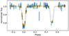 |
Fig. 3. Hipparcos phase-folded photometry, for which the phases were computed from the minimum epoch BJD (Min I)Hp and period PHp given in the text. The Hipparcos measurements are indicated by blue error bars, and the length of the symbol indicates its measurement uncertainty. The reference TESS light curve is indicated by a gray line and orange crosses at the phase of the Hipparcos observations. |
The Gaia epoch photometry was obtained from the ESA Gaia Archive web page. Applying the same treatment as for the Hipparcos light curve to the three Gaia colors, G, Bp, and Rp, we computed three estimates for the Gaia primary minimum and period. The weighted mean of the three minima yields BJD (Min I)G = 2 457 317.7231 ± 0.0016 and PG = 4.93181 ± 2 10−5. The folded light curve is shown in Fig. 4.
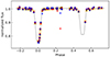 |
Fig. 4. Gaia phase-folded photometry in the G (black), Bp (blue), and Rp (red) filters. The phases were computed from the minimum epoch BJD (Min I)G and period PG given in the text. The symbol size is larger than the measurement uncertainty. The reference TESS light curve is indicated by a gray line and orange crosses at a phase close to the phases of the Gaia observations. The two Gaia points at around phase 0.25 that depart from the general trend might be due to an instrumental issue. |
Paschke & Brat (2006) reported an epoch for a primary minimum in May 1999, BJD (Min I)NSVS = 2 451 325.589 ± 0.005, which they calculated from relative brightness values measured by the Northern Sky Variability Survey (NSVS; Woźniak et al. 2004). The NSVS light curve was approximated with seven harmonic functions, and the minimum was determined at the minimum of the fitted function. We list this minimum in Table A.1 for completeness.
Photometric measurements in V and I filters are given in the archives of the Kamogata-Kiso-Kyoto Wide-field Survey (KWS)1 (Maehara 2014). They cover 2011 to 2024. For each year, we constructed phase diagrams analogous to those for the Hipparcos and Gaia measurements, and we estimated a minimum epoch for each year. The measurement uncertainties are too high and the number of observations in ingress and egress is too low to yield the minimum epoch with sufficient accuracy for the analysis of Sect. 4.2. Therefore, we do not report the KWS minimum epochs.
3. Spectroscopic measurements
V424 Cep was observed on seven nights during June 18–25, 2024 using the high-resolution Manchester Echelle Spectrograph (MES) on the 2.12 m telescope of the Observatorio Astronómico Nacional on the Sierra San Pedro Mártir (OAN-SPM), Baja California, México. The MES is a long-slit single-grating echelle spectrograph that uses interference filters to isolate the order of interest (Meaburn et al. 2003). Spectra were acquired with the Hα and [S II] filters, the latter of which includes the He Iλ6678 line within its bandpass. The spectra of V424 Cep were obtained with a 150 μm slit, which projects to 1.95′′ on the sky. The wavelength calibration was performed using the ThAr arc lamp, which was obtained either immediately before or after each of the object spectra. The flux calibration was made using spectra of BD+25°4655, but without a slit. The calibration file we used is that provided by the European Southern Observatory’s “Standard Stars Catalogues” portal2. The detector was a 2048 × 2048 e2v CCD with 13.5 μm square pixels. The measured FWHM of the arc spectra was 3.0 pixels, implying a spectral resolution (λ/δλ) of 26 000 at Hα.
The data reduction followed standard procedures for long-slit spectra using IRAF (Tody 1986, 1993; Fitzpatrick et al. 2024). Approximately 50 bias images were obtained each night. We subtracted the mean of their over-scan area from the entire image and then combined them to produce a master bias. We subtracted the mean of the over-scan area and the master bias from all other images. No flat-field images were used. The spectra of V424 Cep and BD+25°4655 were extracted to one-dimensional spectra, calibrated in wavelength and flux. For the atmospheric extinction, we adopted the extinction curve from Schuster & Parrao (2001).
The orbital phases were computed with the ephemeris in Table 1. The radial velocities were obtained by measuring the centroid of the lines with Gaussian fits using the IRAF splot routine. There are two sources of uncertainty in these measurements. The first source arises from the uncertainty in the continuum placement, which leads to differences of approximately ±1 km/s in the measured RVs. The second source is due to an asymmetry in the line profiles that does not appear to remain constant from one observation to the next. The effect is most clearly seen in the two spectra of the He I obtained line at orbital phase 0.4. Tables A.2 and A.3 list the centroid of the core of this line for the five observations and indicates that there can be a difference between the core centroid and that of the entire line of 1–7 km/s in the RV measurement of the same spectrum. The largest difference in our limited data set is found in both our orbital phase 0.4 spectra. The difference between the core and the entire line remains relatively constant at ≈2 km/s.
Parameters of a solution of an outer orbit for V424 Cep derived from the measured light time effects for an assumed ω3 = 0.
The observations are summarized in Tables A.2 and A.3, where we list the measured radial velocity of the primary and secondary stars in Cols 6 and 7, respectively, and we show the line profiles in Figs. 5 and 6. The orbital solutions we obtained for each of the two lines are listed in Table 2. As they agree within the uncertainties of the solutions, we combined the Hα and He I measurements into one data set to fit a larger number of measurements . We adopted a period P = 4.93181, an eccentricity e = 0.022, and an angle of periastron ω = 284.46 from the analyses given in the next sections, where the value ω was extrapolated to the spectroscopic observation dates from the analysis given in Sect. 4.1. We fit three parameters to 12 radial velocity measurements of the primary and obtained K1 = 129.4 ± 1.6 km/s, V0 = −19.9 ± 1.0 km/s, and E0 = 60 484.126 ± 0.008, where E0 is the JD of the periastron passage. For the fit to the radial velocity measurements of the secondary, we adopted V0 and E0 as given above because the measurements of the radial velocities of the secondary have larger uncertainties.
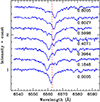 |
Fig. 5. Spectra in the Hα region stacked from bottom to top in order of increasing orbital phase, which is indicated. The vertical line indicates the laboratory wavelength of Hα. No heliocentric correction was applied. |
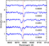 |
Fig. 6. Normalized spectra in the He I λ6678 region stacked from bottom to top in order of increasing orbital phase, which is indicated. The vertical line indicates the laboratory wavelength of the line. No heliocentric correction was applied. |
Radial velocity orbital solutions for V424 Cep.
Figure 7 illustrates the common radial velocity solutions for both lines in the upper and the O–C values in the lower panel. The standard deviations in O–C for the primary are σ1 = 2.8 km/s, and the standard deviation for the secondary is σ2 = 9 km/s. Thus, the empirical uncertainties of the radial velocity measurements are significantly larger than the uncertainties estimated for the measurements.
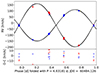 |
Fig. 7. Orbital solution for the measured radial velocities of V424 Cep. The blue symbols are used for the H#x03B1; measurements, and the red symbols show the He I λ6678 measurements. The dashed black curves indicate the solution with e = 0. |
The radial velocity amplitudes allowed us to estimate the orbital separation, mass ratio, and masses: asini = 30.0 ± 0.5 R⊙, q = 0.72 ± 0.03, (M1 + M2)sin3i = 15.0 ± 0.7 M⊙, M1sin3i = 8.7 ± 0.5 M⊙, and M2sin3i = 6.3 ± 0.4 M⊙.
4. Apsidal period and light time effect
4.1. Apsidal motion
The periods derived from the primary and secondary minima differ by P1 − P2 = 8.0 10−6 ± 2.8 10−6 d, which is a difference on the 3σ level. This implies that the location of the periastron has a measurable apsidal motion. This is confirmed by the slope of (T2 − T1)i, which is the difference between successive primary and secondary minima, as shown in Fig. 8. A change in the difference is obvious as T2 − T1 − P/2 changes from 0.012 d at the beginning of the TESS data set to 0.014 d at the end. This trend is also visible in Fig. 2, but in this figure, the effect of the light time effect dominates. The determination of the apsidal motion from T2 − T1 is independent of the influence of the light time effect, and the slope is
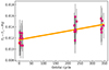 |
Fig. 8. T2 − T1 as a function of the orbital cycle. |
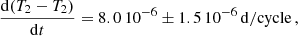
which allowed us to compute
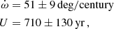
by using Eq. (7) of Baroch et al. (2021), and using the values of the orbital parameters ω, i, and e determined in Sect. 6 to compute the coefficients in the equation, which depend on knowing these three parameters. The given statistical uncertainty does only include the uncertainties of the measurements and it is assumed that the apsidal motion is constant. Because the outer orbit may be highly eccentric (see Sect. 4.2), the apsidal motion might not be constant in time because of the stellar effects.
4.2. Light time effect
The deviations from a linear ephemeris of the minima indicates the light time effect of an outer orbit. The differences of all observed epochs minus an epoch calculated using T0corr and Ps from Table 1 are plotted in Fig. 9. The O–C values of the primary minima are not on a straight line, but there is a scatter of about ±0.02 d, which is larger than the uncertainties of the measured minimum epochs. A conclusive explanation cannot be made without knowing the long-term behavior of the secondary minima. However, because the timescale of the apsidal period derived in Sect. 4.1 is far longer, longer by an order of magnitude than the possible period suggested by Fig. 9, the most likely explanation involves a light time effect associated with an outer orbit.
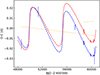 |
Fig. 9. Values of the observed times of eclipse minima minus the values of those computed with a light time effect with the parameters given in Table 1 plotted as a function of time. The blue O–C symbols correspond to the primary eclipse and the red symbols correspond to secondary eclipse. The symbol size indicates the uncertainty as given in Table A.1. The dashed blue and red lines are possible solutions given by the light time equation. The offset between the solutions is due the time difference by which the secondary minimum lags P/2 in the phased orbit. The dotted yellow lines indicates the O–C trends of the primary and secondary eclipses, corrected for the light time effect. |
The equation for a variation in eclipse epochs that is caused by a light time effect of a binary orbit was developed by Woltjer (1922), and the common notation for the parameters can be found, for example, in Irwin (1952), Mayer (1990). The amplitude A with units of light-day was used for half the difference of the maximum O-C-deviations over an orbit, which yielded the line-of-sight semimajor axis of an elliptic orbit 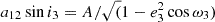 . Here, e3 is the eccentricity of the outer orbit, and ω3 is the corresponding argument of periastron.
Table 1 gives a likely solution for the outer orbit; another possible solution has an amplitude and period that are about twice as large. The given solution for the primary minima is indicated with the dashed blue line in Fig. 9. A highly eccentric orbit is most likely, but with the current data, an eccentricity and the epoch of periastron of the outer orbit are only roughly defined. As there are no measurements of the secondary minima before the TESS observations, the same light time effect solution for the secondary eclipse was adopted as obtained for the primary minima. The two dashed lines indicate the trends of the primary and secondary minimum periods, P1 and P2, corrected for the light time effects.
The amplitude of the light time effect, A, and the eccentricity of the outer orbit e3 given in Table 1 yield a12sini3 = 3.6 AU, which in turn gives the mass function of the third object,

The sum of the masses M1 and M2 is known from Sect. 3 to be 15 M⊙, which yields for the mass of the third object M3 ≈ 4 M⊙, with considerable uncertainties of several M⊙ because the solution for the outer orbit is uncertain. Kervella et al. (2019) computed a proper motion anomaly from Gaia DR2 and Hipparcos measurements and deduced the presence of a third component with an estimated mass 0.4 M⊙ object. The authors had to guess the period and mass of the eclipsing binary pair, and the discrepancy between this mass value and ours is therefore not significant. The existence of a proper motion anomaly, however, supports the interpretation that the deviations of the minimum timings from a linear ephemeris are due to a light time effect.
5. The pulsation periods
In Fig. 10 the two eclipses are shown. The pulsations clearly continue during both eclipses. This means that the primary, the larger and brighter of the two eclipsing stars, is pulsating. Fig. 11 shows the periodograms of the light curves. The green line illustrates that the dominating periods are due to the stellar eclipses. When the eclipses are masked out, the periodogram shows the shape given by the blue line. The periodic signatures of the orbit are still visible, but around periods of 0.17 d, several amplitudes are not reduced. This indicates that there are multiple pulsation periods.
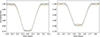 |
Fig. 10. Light curves of V424 Cep of sector 56 (blue dots) and sector 57 (orange dots) folded with the orbital period (Eq. (1)). Left: Primary minimum (Min I) with the smaller and cooler star in front. Right: Secondary minimum (Min II) with the larger and hotter star completely eclipsing the secondary. |
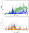 |
Fig. 11. Periodograms of the light curves. Top panel: Periodogram based on all data (green line), and periodogram without the eclipses (blue line). Bottom panel: As the upper panel, but plotted against frequency. The orange line marks the periodogram after the masked light curve was divided by the dominating pulsation period. |
The three strongest pulsation periods in 2019 (sectors 15–17), 2022 (sectors 56–57), and 2024 (sectors 76–77) are given in Table 3. For each interval, the periods were calculated as implemented in the package Lightkurve (Lightkurve Collaboration 2018) using the Lomb-Scargle method and an oversample factor of 10. We also calculated the periodogram for the full light time-series, including all observed sectors, in order to determine whether the oscillations are phase stable. The differences in the period frequencies in Table 3 are not significant and result from differences in sampling and from the length of the three time series.
Pulsation periods, Posc, and amplitudes.
The window function introduced by the periodic data gaps of the masked eclipses produce aliases. These were removed by iteratively dividing the residual time series by a sinusoidal model of the pulsation. This is illustrated in the bottom panel of Fig. 11. After dividing by the dominating period, many of the relatively strong amplitudes shown in blue disappear, and only the peaks drawn in orange remain. The fourth largest period amplitude is at a frequency that had a much stronger period before dividing by the dominating period, and it is likely a remnant of imperfectly removed side peaks of the dominating pulsations. It is unclear whether more than two or three oscillation periods are active. However, there clearly is more than one pulsation period because the amplitudes of the pulsations change visibly in the bottom panel of Fig. 1 and beat from the oscillations, which are close in frequency.
Further investigations showed that the oscillations are stable in frequency, phase, and amplitude for the two strongest modes. The third strongest is also stable in frequency and phase, but its amplitude is reduced by a factor of three in 2022 (sectors 56–57) compared to 2019, and it is no longer among the ten strongest periods in 2024 (sectors 76–77). This change is significant.
In Fig. 12 the light curves are shown phased with 57 times the dominating pulsation period. The difficulty is that when the light curves are folded with one of the pulsation periods, then the pulsation shape is modulated in strength by the other pulsation periods and by the light curve shape between the eclipses, the latter of which varies by about 1% because of the elliptical shape of the primary and because of reflected light (see Sect. 6). This results in a widening of the folded light curve by about half the amplitude of the pulsation. In order to avoid the variation in the orbital light curve, we used a fold period of an integer multiple of the pulsation period that was close to the orbital period, more exactly, to twice the orbital period. To suppress the influence of the other pulsation periods, we binned the folded light curves. The lower panel of Fig. 12 shows that the amplitude of the pulsations remains fairly constant, but some remaining influence of the period beating still remains.
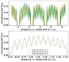 |
Fig. 12. Phase plot of the strongest pulsation. The light curves of the three TESS epochs in 2019, 2022, and 2024 were folded with 57 times the pulsation period Ppuls = 0.17286 d and binned, i.e., averaged. The fold period Pfold = 9.853528 d is close to twice the orbital period, but not exactly equal to it. This brings the eclipses somewhat out of phase, but it is accurate enough to bin the orbital cycle and keeps the intervals of the phased and binned pulsation light curves. The lower panel shows a portion of the phased and binned light curves of the upper panel. |
Based on the analysis of the observed pulsation timings compared to the computed minimum epochs, the scatter, that is, the standard deviation of the O–C values about a linear trend, is ±5 min. However, the O–C values exhibit systematic apparently sinusioidal-like variations with a timescale of about 2 days and amplitudes up to 10 min. As the primary star has a Roche shape, its radius varies, and therefore, we suspect that the systematic deviations might be a variation in the pulsation period. This would imply that the pulsation periods vary on an orbital timescale. Thus, the O-C analysis does not yield another estimate of the light time effect discussed in Sect. 4.2.
6. Fit to the light curve and spectral energy distribution
In the previous sections, we used the radial velocity curves to derive the stellar masses. We also used the eclipse-timing data to show that V424 Cep has a third component in a wide, highly eccentric orbit. In this section, we perform a fit to the eclipse light curve and the spectral energy distribution that is available from archival data. Combined with the results of the previous sections, this fully characterizes the system. It is interesting to note, however, that such a complete set of observations is only rarely available, and the large majority of pulsating stars are characterized on the basis of photometry alone. Hence, we consider it illustrative to first discuss the light curve and SED in a context in which the knowledge we gained from the spectroscopic and O − C analyses is first ignored.
The light curve shows partial eclipses with depths of 24% and 19% with a flat central eclipse. An analysis of the eclipses allowed us to determine the inclination, the radii of the two stars relative to the semimajor axis, the ratio of the brightness temperatures in the TESS passband, and the ratio of the stellar masses. Thus, the absolute stellar properties cannot directly be derived from the light curve alone, and the individual stellar temperatures and the absolute values of the radii therefore remain undetermined in the light-curve analysis. We show in Fig. 13 the light curve that we calculated with PHOEBE, version 2.4.4 (Conroy et al. 2020), without a third-light contribution based on the parameters listed in Table 4.
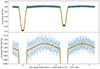 |
Fig. 13. Light curves of sectors 15 and 17 (blue dots) with a time resolution of 2 min, folded with the orbital period. The orange line denotes the folded light curve binned to 15 min steps. The black line is the result of the optimized PHOEBE fit. |
Properties of V424 Cep derived from the light-curve modeling for a zero contribution by third light and for a 15% contribution.
Using the Nelder-Mead optimizer, we fit six parameters to the observed phased light curve: the ratio of the stellar temperatures T2/T1, the relative radii R1/a and R2/a, the inclination i, the eccentricity e, and the angle ω, for an adopted stellar temperature of the primary, T1, a given ratio of the stellar masses q = M2/M1, and a specified projected semimajor axis asini. The atmospheres and their limb darkening were represented by Kurucz atmospheres models, and the reflection efficiency was set to one. The stars were computed in Roche mode using 500 triangles. The parameters we obtained from fitting the light curve are listed in Table 4 for two choices of a third-light contribution, 0% and 15%.
In order to derive the temperature of the brighter star, we compared the computed energy distributions with the observed spectral energy distribution given by photometric measurements as downloaded from the SIMBAD database (Wenger et al. 2000). This database refers to the 2MASS sky survey (Skrutskie et al. 2006) for the J, H, Ks measurements and to the Gaia DR3 data release (Riello et al. 2021) for the Bp, G, Rp values. The absolute fluxes of the Gaia low-resolution XP spectrum (De Angeli et al. 2023) contradict the Gaia photometric fluxes, and we scaled the Gaia spectrum by 0.95 so that it agreed with the Gaia photometry. Figure 14 shows that a two-star composite spectrum with a primary spectrum of T1 = 17 000 ± 1000 K fits the Balmer decrement. Temperatures that deviate by more than 1000 K can be excluded. The companion must have a cooler temperature.
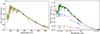 |
Fig. 14. Measured spectral energy distribution of V424 Cep as given by the scaled Gaia XP spectrum (green curve with error bars) and fluxes from Bp, G, Rp, J, H, and K photometry (dots), fit with a two-star composite spectrum as described in the text (orange line). This fit spectrum is for a primary effective temperature T1 = 17 000 K, reddened by EB − V = 0.645, and a radius R1 = 7.5. Left panel: Composite spectra for a primary T1 = 15 000 K and 19 000 K (magenta dots), each with a 2000 K lower temperature for the secondary. The lower and higher temperature spectra are reddened by EB − V = 0.64 and 0.67, respectively. Right panel: Composite spectrum (dashed gray) comprised of three spectra and reddened by EB − V = 0.7 (using R = 3.0), which is almost identical to the orange line in the left panel. The primary has a temperature of T1 = 21 000 K (dotted blue line), the secondary of T2 = 19 000 K (dotted green line), and the third-light spectrum has T3 = 10 000 K with 15% of the total flux at the TESS passband (dotted red line). |
The flux values, in particular, the K magnitude, at the Gaia DR3 distance d = 957 ± 16 pc, allowed us to calculate the radii using the temperatures for T1 = 17 000 K, R1 = 7.78 R⊙ and for T2 = 15 000 K, R2 = 4.05 R⊙, where the temperature ratios and radius ratios were fixed by the light-curve fit. The luminosities of the stars were logL1/L⊙ = 3.7 and logL2/L⊙ = 2.9. These values agree with the Gaia DR3 astrophysical properties (Fouesneau et al. 2023), which give a single OB-star solution for V424 Cep with Teff = 17 070 ± 80 K, R = 8.5 ± 0.13 R⊙, and logg = 3.46 ± 0.01.
After we determined the absolute radii from the observed fluxes and the relative radii from the light-curve fit, we determined the semimajor axis, a = 38 R⊙. This in turn yielded the total mass of the system from Kepler’s third law, M1 + M2 = 29 M⊙ (Eqs. (5)–(165) Lang 1980). The individual masses result from the mass ratio.
When we compare the properties of the stellar pair with standard stellar structure and evolution models, for example, the grids of Ekström et al. (2012), we find that stars with masses higher than M = 15 M⊙ have luminosities logL/L⊙ > 4.2, are much hotter, and have larger radii. The conclusion that would be reached is that the stars are peculiar in that their properties disagree with the standard structure and evolutionary models.
When we adopted the projected semimajor axis asini from Sect. 3, we obtained the masses and radii that are indicated in Fig. 15 by the two thick parts of the black lines. From this figure, we also derived the temperature of the stars, T1 = 21 000 K and T2 = 19 000 K. The flux of the theoretical spectral energy distribution corresponding to a binary system with these properties is only 80% of that which is observed at the K wavelength 2190 nm. This leads to the conclusion that light from a third component needs to be included in the analysis, and it confirms the result of Sect. 4.2.
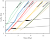 |
Fig. 15. Stellar radii as a function of mass from standard stellar evolution models (Ekström et al. 2012). The slanted colored curves connect the radii of evolutionary models as a function of mass for a temperature as indicated by the label. The full drawn lines show models with rotational mixing of the core, and the dotted lines are from nonration-mixed cores. The thin black curves show the possible mass and radius solutions from the fit to the light curve when the semimajor axis is taken as the free parameter. The upper black curve corresponds to the relation between R1 and M1, and the lower black curves corresponds to that of R2 on M2. The thick parts of the black lines indicate the mass range we derived from the spectroscopic observations in Sect. 3. |
It was not possible to fit a PHOEBE light curve to the observations when we imposed a contribution from the third light that was too large, however. This is because the relative radii (R1/a, R2/a) are constrained by the depth of the eclipses together with the time intervals from first to second and second to third contact of the total eclipse. For example, for a deeper primary eclipse, the radius of the secondary star needs to be increased, which means that the radius of the primary must be reduced in order to conserve the sum R1 + R2, which is constrained by the total duration, that is, from first to fourth contact of the eclipses. This in turn increases the time between first and second contact and decreases the time between second and third contact. With these constraints, the observed light curve limits the contribution of third ight to < 20%. A contribution of 15%, for example, is possible, and we list this PHOEBE solution in Table 4.
A second effect of adding a third-light contribution is that a temperature determination from the Balmer decrement is no longer possible. When we add a star that is cooler than the secondary, the overall Balmer decrement is larger, which can be compensated for by making the primary hotter. As demonstrated in the right panel of Fig. 14, a combination of three spectra with T1 = 21 000 K, T2 = 19 000 K, and T3 = 10 000 K fits the observed Balmer decrement. This solution is not unique, and the temperature of the primary cannot be uniquely determined from the spectral energy distribution without knowing the temperature of the third object, but a primary temperature of about T1 ≈ 21 000 ± 2000 K is likely. A hotter primary implies according to Fig. 15 that its radius is larger, which in turn yields a smaller required amount of flux contribution from a third object. In the example shown in the right panel of Fig. 14, the third-light contribution is 16% of the total light in the TESS wavelength band and 22% in the K band.
7. Discussion
Combining the results of the spectroscopic radial velocity measurements (Sect. 3) with the analysis of the light (Sect. 6), we obtained the stellar properties listed in Table 5. The uncertainties are dominated by the accuracy with which the semimajor axis is known. The inclination derived in Sect. 6 depends on the third-light contribution, which is about 10% to 20%. This excludes a zero contribution from third light. The value for sin3i differs by less than 0.5% from 1 for all cases, and the relative radius dimensions derived from fitting the light curve are also within 1%. Thus, the uncertainties of the light-curve fit do not contribute much to the overall uncertainties of the stellar parameters.
Stellar properties of V424 Cep.
According to Stankov & Handler (2005), several classes of pulsating variables with spectral types B0 – B2.5 exist that lie on the pulsational instability strip. In particular, the β Cepheid-type variables have pulsation periods 0.10–0.22 d, most are of spectral type B1-B2, and they are on or close to the main sequence. Their photometric variation amplitudes lie in the approximate range of 5–90 mmag, the masses are in the range 8–17 M⊙, the luminosities are in the range 3.8–4.6 L⊙, and log(Teff) lies between ≈4.2 to 4.45. By comparing these ranges with the properties of V424 Cep in Table 5, we conclude that the primary component in V424 Cep is a β Cep pulsator.
Another feature of these variables is that their RV variations are associated with the pulsations, which can be as large as 20 km/s, as exemplified by σ Sco (Tkachenko et al. 2014). Our limited set of spectra includes only two observations that were obtained at the same orbital phase, and these do indeed have significantly different He I λ6678 profiles and radial velocity measurements. Another well-known β Cep star is α Vir. Its orbital period and effective temperature are similar to those of V424 Cep, and it shows remarkable line profile variability, including line asymmetries, which affect the RV measurements (Harrington et al. 2016). It is also interesting to note that the α Vir primary is in supersynchronous rotation. In the case of V424 Cep, the primary and secondary both appear to have supersynchronous rotation, even thought these short-period systems are expected to be tidally locked.
Stankov & Handler (2005) proposed a definition of the β Cep-type variables based on theoretical consideration: The radial velocity and/or line profile variations in these stars are caused by low-order pressure and gravity-mode pulsations. Harrington et al. (2009) and Harrington et al. (2016) showed that the observed line profile variability in α Vir could be reproduced using an ab initio calculation of tidally induced pulsations. Tkachenko et al. (2016) attributed only one of the pulsation modes to tidal effects. The system V424 Cep can be used to further study the details of the relation between tidally excited and normal pulsations modes. β Cep-type variables in eclipsing binary systems have been relatively rare, as Eze & Handler (2024) have only recently announced the discovery with TESS of 78 pulsators of the β Cepheid-type in eclipsing binaries, 59 of which are new discoveries.
Finally, it is interesting to note that Kahraman Aliçavuş et al. (2024) argued that most stars that were proposed to be pulsators outside well-established instability domains are misclassified. They also suggested that the existence of possible classes outside the theoretical instability strips, such as the “Maia variables”, is questionable. Our conclusion for V424 Cep agrees with this suggestion.
8. Conclusions
We measured the epochs of the minima in the TESS light curves of V424 Cep and derived precise orbital periods for the primary and secondary minima. Their difference revealed an apsidal motion with a period of about 700 yr. The addition of earlier minima observed by Hipparcos, Gaia, and ground-based observations yielded a fast change in the apsidal period due to a light-time effect from an outer orbit in a hierarchical triple system. The third-light component contributes no more than 15% of the total light of the system in the TESS wavelength band, and it contributes 20% in the K band.
The analyses of the V424 Cep light curve, radial velocity curves, energy distribution, and absolute flux showed that the masses of the binary pair are 8.7 M⊙ and 6.3 M⊙, their radii are 6.0 R⊙ and 3.5 R⊙, and the luminosities are 3.80 L⊙ and 3.11 L⊙. The TESS light curve oscillates with a dominant period of 0.17 d. These oscillations are coherent throughout the orbital cycles with a stable amplitude, except during the (partial) eclipse of the primary star. This indicates that it is the pulsator. Its temperature is 21 000 K. These properties clearly fall within the range found for β Cepheid variables, and we therefore conclude that the pulsator is a β Cepheid variable. Its pulsations are therefore as expected for this type of object. The dominant pulsation period is close to an integral 57:2 ratio, the significance of which is not clear.
Eze & Handler (2024) noted that binary β Cep stars are rare. This highlights the importance of V424 Cep for the study of pulsating variables.
9. Data availability
The spectra shown in Figs. 5 and 6 are available at the CDS via anonymous ftp to https://cdsarc.cds.unistra.fr (130.79.128.5) or via https://cdsarc.cds.unistra.fr/viz-bin/cat/J/A+A/693/A103.
Acknowledgments
This research has made use of the VizieR and SIMBAD catalogue access tools, CDS, Strasbourg, France (Ochsenbein et al. 2000) and of the NASA/IPAC Extragalactic Database (NED), which is funded by the National Aeronautics and Space Administration and operated by the California Institute of Technology. This work has made use of data from the European Space Agency (ESA) mission Gaia (https://www.cosmos.esa.int/gaia), processed by the Gaia Data Processing and Analysis Consortium (DPAC, https://www.cosmos.esa.int/web/gaia/dpac/consortium). Funding for the DPAC has been provided by national institutions, in particular the institutions participating in the Gaia Multilateral Agreement. We thank the daytime and night support staff at the OAN-SPM for facilitating and helping obtain our observations, in particular F. Montalvo, I. Plauchu Frayn, G. Guisa Escobedo, H. Serrano Guerrero, J. Herrera Vázquez, F. Guillen, I. Zavala, T. Calvario, L. Ortiz, T. Verdugo, J. Alonso, and B. Martínez. GK acknowledges funding from UNAM PAPIIT/DGAPA grant IN105723. LFLN acknowledges support by the CONAHCYT scholarship. MGR acknowledges funding from UNAM PAPIIT/DGAPA grants IN111124 and IG101233. Throughout the years, IRAF has also been tirelessly kept alive by a number of volunteers in the astronomy community (including iraf.net and IRAF Community Distribution), providing user support, data reduction tutorials and cookbooks, and maintaining the code. Those efforts are appreciated. NOIRLab IRAF is distributed by the Community Science and Data Center at NSF NOIRLab, which is managed by the Association of Universities for Research in Astronomy (AURA) under a cooperative agreement with the U.S. National Science Foundation. This paper includes data collected with the TESS mission, obtained from the MAST data archive at the Space Telescope Science Institute (STScI). Funding for the TESS mission is provided by the NASA Explorer Program. STScI is operated by the Association of Universities for Research in Astronomy, Inc., under NASA contract NAS 5–26555. This publication makes use of the data from the Northern Sky Variability Survey created jointly by the Los Alamos National Laboratory and University of Michigan. The NSVS was funded by the Department of Energy, the National Aeronautics and Space Administration, and the National Science Foundation.
References
- Aerts, C. 2021, Rev. Mod. Phys., 93, 015001 [Google Scholar]
- Balona, L. A., & Ozuyar, D. 2020, MNRAS, 493, 5871 [CrossRef] [Google Scholar]
- Balona, L. A., Engelbrecht, C. A., Joshi, Y. C., et al. 2016, MNRAS, 460, 1318 [Google Scholar]
- Baroch, D., Giménez, A., Ribas, I., et al. 2021, A&A, 649, A64 [NASA ADS] [CrossRef] [EDP Sciences] [Google Scholar]
- Cannon, A. J., & Pickering, E. C. 1993, VizieR Online Data Catalog: III/135A [Google Scholar]
- Chen, X., Ding, X., Cheng, L., et al. 2022, ApJS, 263, 34 [CrossRef] [Google Scholar]
- Conroy, K. E., Kochoska, A., Hey, D., et al. 2020, ApJS, 250, 34 [Google Scholar]
- De Angeli, F., Weiler, M., Montegriffo, P., et al. 2023, A&A, 674, A2 [NASA ADS] [CrossRef] [EDP Sciences] [Google Scholar]
- Dupret, M. A., Grigahcène, A., Garrido, R., Gabriel, M., & Scuflaire, R. 2004, A&A, 414, L17 [NASA ADS] [CrossRef] [EDP Sciences] [Google Scholar]
- Ekström, S., Georgy, C., Eggenberger, P., et al. 2012, A&A, 537, A146 [Google Scholar]
- ESA 1997, ESA Spec. Publ., 1200 [Google Scholar]
- Eze, C. I., & Handler, G. 2024, ApJS, 272, 25 [NASA ADS] [CrossRef] [Google Scholar]
- Fitzpatrick, M., Placco, V., Bolton, A., et al. 2024, ArXiv e-prints [arXiv:2401.01982] [Google Scholar]
- Fouesneau, M., Frémat, Y., Andrae, R., et al. 2023, A&A, 674, A28 [NASA ADS] [CrossRef] [EDP Sciences] [Google Scholar]
- Gaia Collaboration (Prusti, T., et al.) 2016, A&A, 595, A1 [NASA ADS] [CrossRef] [EDP Sciences] [Google Scholar]
- Gaia Collaboration (De Ridder, J., et al.) 2023a, A&A, 674, A36 [CrossRef] [EDP Sciences] [Google Scholar]
- Gaia Collaboration (Vallenari, A., et al.) 2023b, A&A, 674, A1 [NASA ADS] [CrossRef] [EDP Sciences] [Google Scholar]
- Ginsburg, A., Sipőcz, B. M., Brasseur, C. E., et al. 2019, AJ, 157, 98 [Google Scholar]
- Harrington, D., Koenigsberger, G., Moreno, E., & Kuhn, J. 2009, ApJ, 704, 813 [NASA ADS] [CrossRef] [Google Scholar]
- Harrington, D., Koenigsberger, G., Olguín, E., et al. 2016, A&A, 590, A54 [NASA ADS] [CrossRef] [EDP Sciences] [Google Scholar]
- Irwin, J. B. 1952, ApJ, 116, 211 [Google Scholar]
- Kahraman Aliçavuş, F., Handler, G., Chowdhury, S., et al. 2024, PASA, 41, e082 [CrossRef] [Google Scholar]
- Kazarovets, E. V., Samus, N. N., Durlevich, O. V., et al. 1999, Inf. Bull. Var. Stars, 4659, 1 [Google Scholar]
- Kervella, P., Arenou, F., Mignard, F., & Thévenin, F. 2019, A&A, 623, A72 [NASA ADS] [CrossRef] [EDP Sciences] [Google Scholar]
- Kurtz, D. W. 2022, ARA&A, 60, 31 [NASA ADS] [CrossRef] [Google Scholar]
- Kwee, K. K., & van Woerden, H. 1956, Bull. Astron. Inst. Netherlands, 12, 327 [Google Scholar]
- Lang, K. R. 1980, Astrophysical Formulae. A Compendium for the Physicist and Astrophysicist (Springer) [CrossRef] [Google Scholar]
- Lightkurve Collaboration (Cardoso, J. V. D. M., et al.) 2018, Astrophysics Source Code Library [record ascl:1812.013] [Google Scholar]
- Maehara, H. 2014, J. Space Sci. Inf. Jpn., 3, 119 [Google Scholar]
- Mayer, P. 1990, Bull. Astr. Inst. Czechosl., 41, 231 [NASA ADS] [Google Scholar]
- Meaburn, J., López, J. A., Gutiérrez, L., et al. 2003, Rev. Mex. Astron. Astrofis., 39, 185 [Google Scholar]
- Mowlavi, N., Barblan, F., Saesen, S., & Eyer, L. 2013, A&A, 554, A108 [NASA ADS] [CrossRef] [EDP Sciences] [Google Scholar]
- Ochsenbein, F., Bauer, P., & Marcout, J. 2000, A&AS, 143, 23 [NASA ADS] [CrossRef] [EDP Sciences] [Google Scholar]
- Paschke, A. 2023, BAV J., 79, 1 [NASA ADS] [Google Scholar]
- Paschke, A., & Brat, L. 2006, Open Eur. J. Var. Stars, 23, 13 [NASA ADS] [Google Scholar]
- Petrie, R. M., & Pearce, J. A. 1961, Publ. Dominion Astrophys. Obs. Victoria, 12, 1 [Google Scholar]
- Prša, A., Kochoska, A., Conroy, K. E., et al. 2022, ApJS, 258, 16 [CrossRef] [Google Scholar]
- Ricker, G. R., Winn, J. N., Vanderspek, R., et al. 2015, J. Astron. Telescopes Instrum. Syst., 1, 014003 [Google Scholar]
- Riello, M., De Angeli, F., Evans, D. W., et al. 2021, A&A, 649, A3 [NASA ADS] [CrossRef] [EDP Sciences] [Google Scholar]
- Schuster, W. J., & Parrao, L. 2001, Rev. Mex. Astron. Astrofis., 37, 187 [NASA ADS] [Google Scholar]
- Shi, X.-D., Qian, S.-B., Zhu, L.-Y., et al. 2024, ApJS, 271, 28 [NASA ADS] [CrossRef] [Google Scholar]
- Skrutskie, M. F., Cutri, R. M., Stiening, R., et al. 2006, AJ, 131, 1163 [NASA ADS] [CrossRef] [Google Scholar]
- Stankov, A., & Handler, G. 2005, ApJS, 158, 193 [NASA ADS] [CrossRef] [Google Scholar]
- Swade, D., Fleming, S., Mullally, S., et al. 2019, ASP Conf. Ser., 523, 453 [NASA ADS] [Google Scholar]
- Szewczuk, W., & Daszyńska-Daszkiewicz, J. 2017, MNRAS, 469, 13 [NASA ADS] [CrossRef] [Google Scholar]
- Tkachenko, A., Aerts, C., Pavlovski, K., et al. 2014, MNRAS, 442, 616 [Google Scholar]
- Tkachenko, A., Matthews, J. M., Aerts, C., et al. 2016, MNRAS, 458, 1964 [NASA ADS] [CrossRef] [Google Scholar]
- Tody, D. 1986, SPIE Conf. Ser., 627, 733 [Google Scholar]
- Tody, D. 1993, ASP Conf. Ser., 52, 173 [NASA ADS] [Google Scholar]
- Virtanen, P., Gommers, R., Oliphant, T. E., et al. 2020, Nat. Methods, 17, 261 [Google Scholar]
- Wenger, M., Ochsenbein, F., Egret, D., et al. 2000, A&AS, 143, 9 [NASA ADS] [CrossRef] [EDP Sciences] [Google Scholar]
- Woltjer, J. J. 1922, Bull. Astron. Inst. Netherlands, 1, 93 [NASA ADS] [Google Scholar]
- Woźniak, P. R., Vestrand, W. T., Akerlof, C. W., et al. 2004, AJ, 127, 2436 [Google Scholar]
Appendix A: Minima epochs of V424 Cep
Table A.1 lists minima epochs of V424 Cep. Tables A.2 and A.3 report the measured radial velocities.
Minima epochs of V424 Cep.
SPM spectroscopic observations and measured radial velocities of the Hα line.
SPM spectroscopic observations and measured radial velocities of the He I λ6678 line.
All Tables
Parameters of a solution of an outer orbit for V424 Cep derived from the measured light time effects for an assumed ω3 = 0.
Properties of V424 Cep derived from the light-curve modeling for a zero contribution by third light and for a 15% contribution.
SPM spectroscopic observations and measured radial velocities of the He I λ6678 line.
All Figures
|
Fig. 1. Light curves of V424 Cep observed by the TESS satellite. Top: 79 d of the observations in sectors 15–17 (August 15, 2019, to October 7, 2019). Bottom: 6 d extract from the sector 56 observations (September 2022) plotted with the full time resolution of 2 min. The symbol size shows the precision of the individual measurements. The vertical scale is chosen to illustrate the pulsations, and it therefore truncates the eclipses. |
| In the text | |
|
Fig. 2. Observed minus computed epochs of primary minima (blue) and secondary minima (orange) using the reference ephemeris of Eq. (1). The mean deviation of the secondary minima from Eq. (1), which is <O−C>2 = 17 min, was subtracted to facilitate the comparison of its behavior with that of the primary minima. Each panel corresponds to a different TESS observation epoch, which are sectors 15–17, 56–57, and 76–77. |
| In the text | |
|
Fig. 3. Hipparcos phase-folded photometry, for which the phases were computed from the minimum epoch BJD (Min I)Hp and period PHp given in the text. The Hipparcos measurements are indicated by blue error bars, and the length of the symbol indicates its measurement uncertainty. The reference TESS light curve is indicated by a gray line and orange crosses at the phase of the Hipparcos observations. |
| In the text | |
|
Fig. 4. Gaia phase-folded photometry in the G (black), Bp (blue), and Rp (red) filters. The phases were computed from the minimum epoch BJD (Min I)G and period PG given in the text. The symbol size is larger than the measurement uncertainty. The reference TESS light curve is indicated by a gray line and orange crosses at a phase close to the phases of the Gaia observations. The two Gaia points at around phase 0.25 that depart from the general trend might be due to an instrumental issue. |
| In the text | |
|
Fig. 5. Spectra in the Hα region stacked from bottom to top in order of increasing orbital phase, which is indicated. The vertical line indicates the laboratory wavelength of Hα. No heliocentric correction was applied. |
| In the text | |
|
Fig. 6. Normalized spectra in the He I λ6678 region stacked from bottom to top in order of increasing orbital phase, which is indicated. The vertical line indicates the laboratory wavelength of the line. No heliocentric correction was applied. |
| In the text | |
|
Fig. 7. Orbital solution for the measured radial velocities of V424 Cep. The blue symbols are used for the H#x03B1; measurements, and the red symbols show the He I λ6678 measurements. The dashed black curves indicate the solution with e = 0. |
| In the text | |
|
Fig. 8. T2 − T1 as a function of the orbital cycle. |
| In the text | |
|
Fig. 9. Values of the observed times of eclipse minima minus the values of those computed with a light time effect with the parameters given in Table 1 plotted as a function of time. The blue O–C symbols correspond to the primary eclipse and the red symbols correspond to secondary eclipse. The symbol size indicates the uncertainty as given in Table A.1. The dashed blue and red lines are possible solutions given by the light time equation. The offset between the solutions is due the time difference by which the secondary minimum lags P/2 in the phased orbit. The dotted yellow lines indicates the O–C trends of the primary and secondary eclipses, corrected for the light time effect. |
| In the text | |
|
Fig. 10. Light curves of V424 Cep of sector 56 (blue dots) and sector 57 (orange dots) folded with the orbital period (Eq. (1)). Left: Primary minimum (Min I) with the smaller and cooler star in front. Right: Secondary minimum (Min II) with the larger and hotter star completely eclipsing the secondary. |
| In the text | |
|
Fig. 11. Periodograms of the light curves. Top panel: Periodogram based on all data (green line), and periodogram without the eclipses (blue line). Bottom panel: As the upper panel, but plotted against frequency. The orange line marks the periodogram after the masked light curve was divided by the dominating pulsation period. |
| In the text | |
|
Fig. 12. Phase plot of the strongest pulsation. The light curves of the three TESS epochs in 2019, 2022, and 2024 were folded with 57 times the pulsation period Ppuls = 0.17286 d and binned, i.e., averaged. The fold period Pfold = 9.853528 d is close to twice the orbital period, but not exactly equal to it. This brings the eclipses somewhat out of phase, but it is accurate enough to bin the orbital cycle and keeps the intervals of the phased and binned pulsation light curves. The lower panel shows a portion of the phased and binned light curves of the upper panel. |
| In the text | |
|
Fig. 13. Light curves of sectors 15 and 17 (blue dots) with a time resolution of 2 min, folded with the orbital period. The orange line denotes the folded light curve binned to 15 min steps. The black line is the result of the optimized PHOEBE fit. |
| In the text | |
|
Fig. 14. Measured spectral energy distribution of V424 Cep as given by the scaled Gaia XP spectrum (green curve with error bars) and fluxes from Bp, G, Rp, J, H, and K photometry (dots), fit with a two-star composite spectrum as described in the text (orange line). This fit spectrum is for a primary effective temperature T1 = 17 000 K, reddened by EB − V = 0.645, and a radius R1 = 7.5. Left panel: Composite spectra for a primary T1 = 15 000 K and 19 000 K (magenta dots), each with a 2000 K lower temperature for the secondary. The lower and higher temperature spectra are reddened by EB − V = 0.64 and 0.67, respectively. Right panel: Composite spectrum (dashed gray) comprised of three spectra and reddened by EB − V = 0.7 (using R = 3.0), which is almost identical to the orange line in the left panel. The primary has a temperature of T1 = 21 000 K (dotted blue line), the secondary of T2 = 19 000 K (dotted green line), and the third-light spectrum has T3 = 10 000 K with 15% of the total flux at the TESS passband (dotted red line). |
| In the text | |
|
Fig. 15. Stellar radii as a function of mass from standard stellar evolution models (Ekström et al. 2012). The slanted colored curves connect the radii of evolutionary models as a function of mass for a temperature as indicated by the label. The full drawn lines show models with rotational mixing of the core, and the dotted lines are from nonration-mixed cores. The thin black curves show the possible mass and radius solutions from the fit to the light curve when the semimajor axis is taken as the free parameter. The upper black curve corresponds to the relation between R1 and M1, and the lower black curves corresponds to that of R2 on M2. The thick parts of the black lines indicate the mass range we derived from the spectroscopic observations in Sect. 3. |
| In the text | |
Current usage metrics show cumulative count of Article Views (full-text article views including HTML views, PDF and ePub downloads, according to the available data) and Abstracts Views on Vision4Press platform.
Data correspond to usage on the plateform after 2015. The current usage metrics is available 48-96 hours after online publication and is updated daily on week days.
Initial download of the metrics may take a while.