| Issue |
A&A
Volume 693, January 2025
|
|
|---|---|---|
| Article Number | A286 | |
| Number of page(s) | 16 | |
| Section | Interstellar and circumstellar matter | |
| DOI | https://doi.org/10.1051/0004-6361/202450260 | |
| Published online | 24 January 2025 | |
Intermediate mass T Tauri disk masses and a comparison to their Herbig disk descendants
1
Leiden Observatory, Leiden University,
PO Box 9513,
2300 RA
Leiden,
The Netherlands
2
Max-Planck-Institut für Astronomie,
Königstuhl 17,
69117
Heidelberg,
Germany
3
Anton Pannekoek Institute for Astronomy, University of Amsterdam,
PO Box 94249,
1090 GE,
Amsterdam,
The Netherlands
4
Max-Planck-Institut für Extraterrestrische Physik,
Giessenbachstrasse 1,
85748
Garching,
Germany
5
European Southern Observatory,
Karl-Schwarzschild-Strasse 2,
85748
Garching,
Germany
6
Institute for Astronomy, University of Hawaii,
Honolulu,
HI
96822,
USA
7
School of Natural Sciences, Center for Astronomy, University of Galway,
Galway
H91 CF50,
Ireland
★ Corresponding author; This email address is being protected from spambots. You need JavaScript enabled to view it.
Received:
5
April
2024
Accepted:
12
November
2024
Abstract
Context. Herbig disks are prime sites for the formation of massive exoplanets and looking into the precursors of these disks can offer clues for determining planet formation timescales. The precursors of Herbig stars, called intermediate-mass T Tauri (IMTT) stars, have spectral types later than F, but stellar masses between 1.5 and 5 M⊙. These stars will eventually become Herbig stars of spectral types A and B.
Aims. The aim of this work is to obtain the dust and gas masses and radii of all IMTT disks with ALMA archival data. The obtained disk masses are then compared to Herbig disks and T Tauri disks and the obtained disks sizes to those of Herbig disks.
Methods. ALMA Band 6 and 7 archival data were obtained for 34 IMTT disks with continuum observations, 32 of which have at least 12CO, 13CO, or C18O observations, but with most of them at quite shallow integrations. The disk integrated flux together with a stellar luminosity-scaled disk temperature were used to obtain a total disk dust mass by assuming optically thin emission. Using thermochemical Dust And LInes (DALI) models drawn from previous works, we also obtained gas masses of 10 out of 35 of the IMTT disks based on the CO isotopologues. From the disk masses and sizes, we obtained the cumulative distributions.
Results. The IMTT disks in this study have the same dust mass and radius distributions as Herbig disks. The dust mass of the IMTT disks is higher compared to that of the T Tauri disks, as also found for the Herbig disks. No differences in dust mass were found for group I versus group II disks, in contrast to Herbig disks. The disks for which a gas mass could be determined display a similarly high-mass as to the Herbig disks. Comparing the disk dust and gas mass distributions to the mass distribution of exoplanets shows that there also is not enough dust mass in disks around intermediate-mass stars to form massive exoplanets. On the other hand, there is more than enough gas to form the atmospheres of exoplanets.
Conclusions. We conclude that the sampled IMTT disk population is almost indistinguishable compared to Herbig disks, as their disk masses are the same, even though the former objects are younger. Based on this study, we conclude that planet formation is already well underway in these objects and, thus, planet formation is expected to start early on in the lifetime of Herbig disks. Combined with our findings on group I and group II disks, we conclude that most disks around intermediate-mass pre-main sequence stars converge quickly to small disks, unless they are prevented from doing so by a nearby massive exoplanet.
Key words: surveys / protoplanetary disks / stars: early-type / stars: pre-main sequence / stars: variables: T Tauri, Herbig Ae/Be / submillimeter: planetary systems
© The Authors 2025
 Open Access article, published by EDP Sciences, under the terms of the Creative Commons Attribution License (https://creativecommons.org/licenses/by/4.0), which permits unrestricted use, distribution, and reproduction in any medium, provided the original work is properly cited.
This article is published in open access under the Subscribe to Open model.
Open Access funding provided by Max Planck Society.
1 Introduction
Herbig disks are planet-forming disks around pre main-sequence stars called Herbig stars and characterized by spectral types of B, A, and F, and stellar masses of 1.5 M⊙ to 10 M⊙ (e.g., Herbig 1960; Brittain et al. 2023). These disks are the precursors of famous directly imaged planetary systems such as HR 8799 (Marois et al. 2008, 2010), β Pic (Lagrange et al. 2010), and 51 Eri (Chauvin et al. 2017), and host some of the first kinematically detected planets (Pinte et al. 2018; Izquierdo et al. 2023). How these planets have formed is not known, but we do know from exoplanet statistics that the prevalence of giant planets is highest around intermediate-mass stars (e.g., Johnson et al. 2007, 2010; Nielsen et al. 2019; Fulton et al. 2021). Comparing dust structures and planet occurrence rates indeed reveals a positive correlation between the two, along with an increase in the prevalence of dust structures with stellar mass (van der Marel & Mulders 2021). Hence, Herbig disks are an important piece of the planet formation puzzle.
However, Herbig disks are generally quite old (a median age of 6 Myr for Herbig Ae stars, Vioque et al. 2018) and many exhibit structures that are indicative of planet formation, making these some of the most well-known and widely investigated disks (e.g., HD 100546, HD 163296, MWC 480; Fedele et al. 2017; Teague et al. 2018; Öberg et al. 2021; Booth et al. 2023). Planets may already begin forming early on in the lifetime of the disk, as evidenced by an apparent lack of solids in class II disks to form the observed family of giant exoplanets (Manara et al. 2018; Tychoniec et al. 2020), as well as structures are already visible in earlier stages (ALMA Partnership 2015; Segura-Cox et al. 2020). While the recent ALMA large program eDisk (Ohashi et al. 2023) does not show as many substructures in class 0 and class I objects as expected, possibly because these structures have not formed yet or have high continuum optical depth, planetesimals (i.e., the building blocks of planets) are likely to already form in these younger objects (e.g., Drążkowska & Dullemond 2018). Hence, these younger objects still have the capacity to provide insights into planet formation timescales.
In total, around 380 Herbig stars are known (Vioque et al. 2018; Wichittanakom et al. 2020; Guzmán-Díaz et al. 2021; Vioque et al. 2022). In addition, around 1500 more Herbig candidates have been identified by Vioque et al. (2020), so the total population size is expected to be much greater. A recent compilation of all available ALMA archival data out to Orion (~450 pc) has shown that these Herbig disks are more massive in dust mass than the disks around their lower stellar mass counterparts (with spectral type F and later and a stellar mass of ≲1.5 M⊙) called T Tauri stars (Stapper et al. 2022). This feature could naturally result in the higher prevalence of giant exoplanets around higher mass stars (e.g., Johnson et al. 2010). Moreover, the work of Stapper et al. (2024) has indicated that the Herbig disks are much warmer compared to T Tauri disks, causing less CO freeze-out and reprocessing in Herbig disks, in line with thermo-chemical models (Bosman et al. 2018). This makes CO a viable mass tracer in Herbig disks.
However, due to the relatively horizontal pre-main sequence evolutionary tracks in the Hertzsprung–Russell diagram, there are intermediate-mass objects that were not part of the analysis of Stapper et al. (2022, 2024) that have the same stellar mass as Herbig stars, but a spectral type later than F. These are called intermediate-mass T Tauri (IMTT) stars and they are the precursors of Herbig stars. With spectral types of F to K3 and stellar masses between 1.5 and 5 M⊙, they look like T Tauri stars, but exhibit an intermediate mass (Calvet et al. 2004; Valegård et al. 2021). This is shown in the Hertzsprung-Russel diagram in Fig. 1, where the difference in effective temperatures can be seen between the Herbig stars and IMTT stars. As a reference, the 2.5 Myr isochrone is shown, which clearly indicates that the IMTT stars are younger than their Herbig star descendants, although the ages can be relatively uncertain. Valegård et al. (2021) has compiled a sample of 49 IMTTs based on optical photometry. All stars within 500 pc with spectral types ranging from F0 to K3 and with a stellar luminosity of at least 2.1 L⊙ (i.e., M★ ≥ 1.5 M⊙) were selected. The resulting sample, while not as young as class I objects, has a median age of4 Myr, ranging from 0.3 Myr to 9 Myr, based on isochrones. We note that, similarly to the case of the Herbig disks, the IMTT disks are likely biased toward the high accretors and brightest disks (see, e.g., Fig. 1 of Grant et al. 2023). A millimeter study into this sample will give insight into the evolution of the dust and gas around these intermediate-mass objects.
A significant fraction of the IMTTs compiled by Valegård et al. (2021) has ALMA millimeter observations. In this work, we compile the available ALMA data and compare the obtained dust masses to previous works of Herbig disks (Stapper et al. 2022, hereafter S22), as well as the gas masses to Herbig disks (Stapper et al. 2024, hereafter S24) and to T Tauri disks (e.g., Ansdell et al. 2016, 2017; Barenfeld et al. 2016; van Terwisga et al. 2020, 2022; Manara et al. 2023).
In Sect. 2, we set out the data selection and reduction procedures. In Sect. 3, we explore whether new models are needed, compared to the DALI (Bruderer et al. 2012; Bruderer 2013) thermochemical models run for Herbig disks in S24, which can then be used to determine the gas masses from the CO observations. In Sect. 4, we show the resulting continuum and gas images in Sects. 4.1 and 4.2, respectively, obtain a dust mass and dust radius distribution, and compare these with previous works in Sect. 4.3. We explain how we obtained the gas masses and radii in Sect. 4.4 and compare these values to previous works. We discuss these results in Sect. 5, in the context of the Meeus et al. (2001) groups and the evolution of disks around intermediatemass stars in Sect. 5.1, and discuss the implications on planet formation around intermediate-mass stars in Sect. 5.2. Lastly, Sect. 6 summarizes our conclusions.
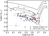 |
Fig. 1 HR-diagram of the Herbig star sample of S22, and the compiled IMTT sample in this work. The effective temperatures and luminosities are taken from Vioque et al. (2018) and Valegård et al. (2021) for the Herbig stars and IMTT stars, respectively. Pre-main sequence tracks of different intermediate-mass stars and an isochrone of 2.5 Myr as the dashed line are taken from Marigo et al. (2017). |
2 Data selection and reduction
Using the IMTTs from Valegård et al. (2021), we obtained all publicly available Band 6 and 7 data on the ALMA archive1 containing continuum, 12CO, 13CO, and C18O observations. There is some overlap between the Herbig disks and IMTTs from Vioque et al. (2018) and Valegård et al. (2021), the former have been used in S22 for Herbig dust masses. These are AK Sco, HD 135344B, HD 142527, and HD 142666 (see Table A.1 for their spectral types). We use the data of these objects as presented in both S22 and S24. Additionally we include recently published ALMA data from the DESTINYS program (e.g., Garufi et al. 2024, Ginski et al. 2024, Valegård et al. 2024) with project code 2021.1.01705.S (P.I.: C. Ginski), along with not-yet-published data with project code 2022.1.01155.S (P.I.: M. Vioque) and ACA data with project codes 2021.2.00005.S and 2022.1.01460.S (both P.I.: J. Williams). The resulting sample of IMTTs exhibits spectral types ranging from A8 to K4. The histograms presented in Fig. 2 show that this range in spectral types overlaps with the late spectral type Herbig stars and the early spectral type T Tauri stars, but that the range in stellar masses is the same as that of the Herbig stars. Also, we refer to Fig. 1 for a comparison between the Herbig stars and the IMTT stars of the sample in S22 and this work, respectively, on the HR-diagram.
When comparing the stellar parameters of the resulting sample of 35 IMTTs to the full sample of Valegård et al. (2021), no significant differences regarding the stellar luminosity and mass were found. Using the Spitzer 30 µm fluxes from Valegård et al. (2021) as a measure of the presence of a disk, no significant differences were found either. A similar comparison can be made for the Herbig disks among the sample of Stapper et al. (2022) and the full sample of Vioque et al. (2018) given in Appendix D of Stapper et al. (2022). No significant differences were found for the Herbig disks in that case either. Still, the samples themselves might be biased toward the highest accretors (Grant et al. 2023) or biased toward the largest and brightest disks of the total population. However, as both the IMTTs and the Herbigs are biased in the same way, comparisons can still be made.
The observing details of the unpublished data can be found in Table 1. In general, the integration times are of the order of minutes, ranging from 1.4 min to 7.5 min. The data were taken in 2022 and 2023, almost all within a year of each other. As project 2021.1.01705.S only covers the continuum and the 12CO line, we supplemented the data with other projects (where possible) to include the 13CO and C18O lines. Specifically for HD 34700 and PDS 277, only the 13CO and C18O data from 2021.2.00005.S were taken, and the 12CO and continuum data were taken from the more sensitive observations of the 12m array.
The 12-m array data were phase self-calibrated based on the continuum data for multiple rounds up until the peak signal-to-noise did not improve compared to the previous round. This increased the peak signal-to-noise (S/N) of 12 of our targets (AK Sco, CR Cha, HD 135344 B, HD 142527, HD 294260, HT Lup, PDS 156, PDS 277, RY Tau, SR 21, SU Aur, and UX Tau). In most cases, one to three rounds were performed, beginning with a solution interval at “inf”and then decreasing by factors of two, which increases the S/N by a factor of 1.7, on average. After the phase calibration, a single round of amplitude calibration was performed as well, which was only applied to SU Aur. The resulting calibration table was applied to the line spectral windows by using the applycal task. For the ACA data, no self-calibration was done. In this work, for T Tau, we only use the continuum data as the CO observations show very complex structures, making it difficult to obtain a good measure of the disk mass and size. For more on the T Tau CO data, we refer to Rota et al. (2022).
For the continuum data, the imaging was done using multifrequency synthesis. The spectral lines were imaged after subtracting the continuum using uvcontsub. Different velocity resolutions were used depending on the dataset. For the imaging, we used multiscale using 0 (point source), 1, 2, 5, 10, and 15 times the size of the beam in pixels (~5 pixels) as the size of the scales. The last three scales were only used if the disk morphology allowed for it. Lastly, for the mosaic data of Brun 656 and HBC 502, we used the product data from the archive. We refer to Table B.1 for the resulting data parameters.
To obtain the disk integrated fluxes, we used the same method as described in S22 and S24, where an increasing aperture size was used to ascertain the maximum amount of disk integrated flux. This method also returns a size of the disk. The found fluxes and sizes are presented in Table A.2.
To obtain the dust masses, we follow previous population studies (see e.g., Miotello et al. 2023 for an overview), using the relationship of Hildebrand (1983) to directly relate the continuum emission to the dust mass, assuming optically thin emission,
 (1)
(1)
Here, Fν is the continuum flux as emitted by the dust in the disk at a distance, d, to the object, and κν is the dust opacity, which is estimated as a power-law taking the form of κν ∝ vβ, equal to 10 cm2 g−1 at a frequency of 1000 GHz (Beckwith et al. 1990). The power-law index, β, is assumed to be equal to 1. Bν(Tdust) is the value of the Planck function at a given dust temperature, Tdust. The dust temperature is given by the relationship of Andrews et al. (2013), which scales the dust temperature by the stellar luminosity in solar luminosities via
 (2)
(2)
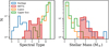 |
Fig. 2 Histogram of the spectral types (left panel) and stellar masses (right panel) of the IMTTs in this work (from Valegård et al. 2021) compared to the Herbig star sample of S22 and references therein, as well as the surveys of Lupus (Ansdell et al. 2016) and Upper Sco (Barenfeld et al. 2016). |
Observing details of the unpublished data.
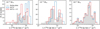 |
Fig. 3 Histogram of the disk integrated C18O luminosities of models run by the thermochemical code DALI for three different disk masses, as indicated in the top-left of each panel. A comparison is done between the models used by S24 (gray), and models for which the stellar effective temperature has been lowered to an IMTT appropriate value either with (red) or without (blue) accretion UV added. The lower effective temperature of the IMTT star increases the C18O luminosity for the lowest mass disks compared to the Herbig disk models, as there is less UV emission and therefore less photodissociation of CO. Adding the accretion UV increases the photodissociation of CO, moving the C18O luminosity back to Herbig disk levels. |
3 Model setup
For the modeling of the CO isotopologues, we used the DALI grid for Herbig disks presented in S24. DALI (Bruderer et al. 2012; Bruderer 2013) is a thermo-chemical code, which takes heating, cooling, and chemical processes into account and uses them to solve for the gas and dust thermal structure of the disk. The models used by S24 use the CO isotopologue chemistry network of Miotello et al. (2016), which includes isotope-selective photodissociation, fractionation reactions, selfshielding, and freeze-out. The models use a parametric description for the density structure, motivated by a viscous accreting disk (Lynden-Bell & Pringle 1974; Hartmann et al. 1998). The vertical gas distribution is given by a Gaussian distribution. The grid run by S24 consists of models with disk masses ranging from 10−5 to 10−0.5 M⊙, have different radial and vertical mass distributions, as well as different stellar luminosities and disk inclinations (see S24 for more details). The models were run until chemical equilibrium was reached at 1 Myr.
T Tauri stars have lower effective temperatures, compared to Herbig stars, resulting in less UV photospheric emission in the former compared to the latter. As accretion contributes significantly to the overall UV budget, UV emission from accretion is added to the stellar spectrum for T Tauri stars (e.g., Miotello et al. 2014, 2016). This is in contrast to Herbig stars, for which the accretion UV is not significant compared to the UV photons already emitted by the star itself (Miotello et al. 2016). Yet, in the case of the IMTTs, accretion UV does significantly add to the overall UV budget.
To test this notion, we compare the grid of models from S24 to two smaller grids of models with the only difference being that an effective stellar temperature of 5500 K and luminosity of 10 L⊙ are used for the IMTT disks based on the values of Valegård et al. (2021), excluding the largest disk models from S24. One grid has accretion UV added and one grid does not. The accretion luminosity is set as 1.5 L⊙, the median value from the works of Calvet et al. (2004), from modeling at wavelengths >2000 Å, and Wichittanakom et al. (2020), from Hα emission. The accretion was added to the stellar spectrum with a blackbody at 104 K. The addition of the accretion UV results in Lfuv/Lbol = 1.1 × 10⁻², compared to Lfuv/Lbol = 1.2 × 10⁻³ without, and Lfuv/Lbol = 7.4 × 10⁻² for the Herbig disks. The addition of the accretion gives a difference of an order of magnitude compared to the case without accretion; this result is similar to the difference between the T Tauri and Herbig disk models of Miotello et al. (2016). Figure 3 compares the resulting disk integrated C18O luminosities of both grids to the Herbig disk grid from S24, raytraced at a distance of 100 pc. Each panel presents a different gas mass, from 10−4 to 10−2 solar masses. The lower effective temperature of the IMTT stars decreases the UV luminosity compared to Herbig stars, which increases the C18O luminosity of the disk for the lowest disk masses due to a decrease in photo-dissociation of CO. As the CO gas becomes optically thin, either due to a larger disk or a lower disk mass, self-shielding becomes less efficient. For the highest disk mass considered in Fig. 3, the disk integrated C18O luminosity is very similar to that of the Herbig disks. When including the accretion UV the C18O luminosity decreases, compensating for the decrease in UV emission due to the lower effective temperature. This effectively moves the distribution back again to that of the Herbig disks. This shows that the Herbig disk models can be used for the IMTT models and hence, we use the same models in this work as was used in S24.
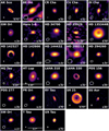 |
Fig. 4 Continuum images of intermediate-mass T Tauri disks with a detection, using a sinh stretch. The size of the image is indicated by the bar of size 100 au on the bottom right of each panel with the corresponding angular size. The beam size is shown as the ellipse on the bottom left of each panel. The group classification can be found in Table A.1. |
4 Results
4.1 Continuum images
Figure 4 presents the continuum images of all IMTTs observed with ALMA. Similar to the observations of Herbig disks in S22, there is a large variety of sizes and structures visible in our set of IMTT observations. The majority of disks are unresolved, but all disks which are resolved exhibit single or multiple rings. In total, 12 disks have resolved observations showing structures, out of the 26 detected disks, this is 46%. This is lower compared to the fraction found by S24, which was 60% (15/25), which is likely due to the lower spatial resolution of the data available in our work and this percentage will increase with higher resolution data. AK Sco, HD 135344B, HD 142527, and HD 142666, which are also classified as Herbig disks, are part of these resolved disks. Removing these disks lowers the number of resolved IMTT disks to 8, showing a clear lack of deep observations toward IMTT disks.
Apart from disks with resolved structures, there are three unresolved disks which are noteworthy. For HD 35929 the data give strong constraints on the size of the dust disk (less than 41 au), while remaining unresolved. In addition, SU Aur and HD 34700, which show extended asymmetric emission in the dust, while the main disk is unresolved. In particular, SU Aur is famous for its large arm in CO due to late-stage infall, which could be related to this asymmetry (Ginski et al. 2021).
There are also multiple stellar systems present in our sample. HD 288313 in particular is a complex system of at least three components (Reipurth et al. 2010). The disk around the A component (the Herbig star) is quite faint in the continuum emission, while one of the other components has a peak flux that is an order of magnitude higher. HT Lup is a triple system, with all three components having clear millimeter continuum emission (Kurtovic et al. 2018). The A component around the Herbig star has the largest disk. In Fig. 4, the B component is also visible, while the C component is outside of the field of view. Lastly, T Tau is a triple stellar system (Köhler et al. 2016).
4.2 Gas images
The moment zero maps of disks for which at least one of the three CO isotopologues are detected are presented in Fig. 5. If one of the isotopologues is detected, the other non-detections are also shown by integrating over the same velocity range as is done for the detected isotopologue. If a panel is empty, no observations of that particular isotopologue are available.
Again, a large variety in structures can be seen. In particular cavities are visible in three of our disks in both 13CO and C18O: HD 135344B, LkHα 330, and HD 142527 (see for more on these disks e.g., van der Marel et al. 2015; Brown et al. 2008; Pinilla et al. 2022; Temmink et al. 2023). This is indicative of deep cavities, where these molecules become optically thin. Apart from cavities other structures are visible as well, in particular envelopes and streamers. These potential streamers and envelopes can be seen in the 12CO emission of GW Ori, T Tau (Rota et al. 2022), and SU Aur (Ginski et al. 2021). This extended emission does pose difficulties in obtaining a measure of the radii and integrated fluxes. HT Lup has large unresolved structures, seen as the large fringe patterns in the observations and strong continuum absorption in the center of the disk (cavitylike appearance in Fig. 5). Other disks with absorption include SR 21 in particular, with strong absorption features on the southwestern side of the disk resulting in an asymmetric appearance in 12CO.
Out of the 31 disks with at least one of the three CO isotopologues available, 16 out of 28 (57%) for which 12CO data are available have a detection, while this is 11 out of 29 (38%) for 13CO, and 10 out of 28 (36%) for C18O. In general, if 13CO is detected, then C18O is detected as well. On the other hand, there are four disks which have 12CO detected, while the other CO isotopologues are not.
4.3 Dust masses and radii
We can obtain cumulative distributions from the dust masses using the lifelines package (Davidson-Pilon et al. 2021), together with the probability distributions by fitting a log-normal distribution (see the left and right panel of Fig. 6 respectively). In addition, the cumulative distribution of the Herbig disks from S22 (with a median age of 5.5 Myr and a median stellar mass of 2 M⊙), and the distributions of the disks in Lupus (1–3 Myr, median stellar mass of 0.24 M⊙, Ansdell et al. 2016) and Upper Sco (5–10 Myr, median stellar mass of 0.26 M⊙, Barenfeld et al. 2016) are also shown.
The distributions of the Herbig dust masses and the IMTT dust masses stand out as very similar. At around 60 M⊕ the IMTT distribution does dip below the Herbig distribution, but is still within the shaded region indicating the 1σ confidence interval. Using a Kolmogorov-Smirnov test using scipy (Virtanen et al. 2020), we can assess whether the distributions are sampled from the same underlying distribution. We obtained a p-value of 0.962, indicating that the null hypothesis is acceptable and that both distributions have the same underlying dust mass distribution.
Following S22, we can obtain the probability distributions by fitting a log-normal distribution to the cumulative distributions using a bootstrapping method with 105 samples. These fits result in the probability distributions shown in the right panel of Fig. 6. The resulting distributions show a clear overlap between the Herbig disks and IMTTs. Table 2 shows the resulting means and standard deviations of the distributions. We include the dust masses of five Herbig disks2 observed with NOEMA from S24; hence, we can see the difference in obtained parameters for the Herbig disk dust mass distribution, compared to the one in S22. Both the mean and the standard deviation of the Herbig disks and IMTTs fall within the given uncertainty intervals. Hence, further supporting the similarities between the two distributions.
Figure 7 presents the cumulative distributions of the R90% dust radii for the IMTT disks and for the Herbig disks (S24). The radii are very similar between the two populations, as was also the case for the dust masses. The largest IMTT disk in our sample is the disk of GW Ori, with a 90% radius of 382 au. The other resolved disks range from 236 au down to 25 au with a median of 69 au. Again using a Kolmogorov-Smirnov test, we can test the null hypothesis of both distributions being sampled from the same populations. Indeed, we cannot reject this null hypothesis based on the resulting p-value of 0.860; hence, the two distributions can be sampled from the same underlying population.
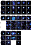 |
Fig. 5 12CO, 13CO, and C18O velocity integrated-intensity maps as obtained with Keplerian masking for all IMTTs which have a detection in at least one of the three isotopologues. An empty panel indicates that no observations are available of that particular isotopologue. |
4.4 Gas masses and radii
In this section, we compare the disk integrated luminosities of the 13CO and C18O isotopologues to the DALI models obtained by S24. This is shown in Fig. 8. In the left panel, the J = 2 − 1 transition is shown, while the right panel shows the J = 3 − 2 transition of the CO isotopologues, for both the observations and the models of S24.
Comparing the observed and modeled 13CO and C18O luminosities as shown in Fig. 8, it is clear that for the detected disks, most are in the optically thick regime similar to the Herbig disks, as the smallest disks are on the bottom left, while the largest disks are on the top right. For the models, the multiple orders of magnitude in disk mass overlap with the same 13CO and C18O fluxes, while for the larger disks the models fan out. The “hook” shape seen for models with the same disk mass are due to an increased disk radius which reduces the self-shielding capacity of the CO molecules, reducing the emission of the C18O first and then the 13CO. We refer to S24 for more details.
For disks in which the CO isotopologues are detected, we obtained the disk mass after selecting models based on the disk and stellar parameters in Table A.1 (see S24 for details on this selection process). The cumulative gas mass and gas-to-dust ratio distributions and their corresponding probability distributions can be found in Fig. 9. We find a gas mass distribution of Log10(Mdisk) = −1.88±0.87 M⊙ for the IMTTs, compared to log10(Mdisk) = −1.55±0.46 M⊙ for the Herbigs. Importantly, while the upper limits for the Herbig disks with non-detections of 13CO and C18O were constraining enough to obtain a limit on the disk mass, the upper limits obtained for the IMTT disks were not. Hence, most have upper limits of the maximum disk mass in the model grid. The obtained gas masses are in general 0.3 dex lower compared to the Herbig disks (see Fig. 9). The distribution is wider and goes toward lower gas masses compared to the Herbig disks.
Combining the gas and dust mass distributions of the IMTT and Herbig disks from Figs. 6 and 9, we obtain two similar gas-to-dust ratio distributions in the bottom row of Fig. 9. Apart from RY Tau, which has a relatively low C18O flux compared to its 13CO flux, all disks show gas-to-dust ratios of at least the ISM value of 100 or higher, with a distribution of Log10(Δɡ/d) = 2.21±0.37 for the IMTTs compared to Log10(Δɡ/d) = 2.48±0.38 for the Herbigs. This is in line with the findings for the Herbig disks in S24. The distribution of the IMTT disks seems to be lower by ~0.2 dex, but this falls within the 1-sigma width of the distributions. Hence, we conclude that there is no indication of the IMTT gas-to-dust ratios being different when compared to the Herbig disks. The fact that high gas-to-dust ratios are found for these disks could be an indication of that the dust masses, as determined via Eq. (1), are underestimated. This could indicate that either the assumption of optically thin emission does not hold, or that the assumed dust opacity is incorrect. Recent works have indeed shown that dust masses can be underestimated by up to a factor of ~7 due to these effects (e.g., Liu et al. 2022; Xin et al. 2023; Savvidou & Bitsch 2025).
The dust and gas 12CO 90% radii are presented in Fig. 10, where the radii are compared to those of the Herbig disks (S22 and S24). The dust radial drift dominated limit from Trapman et al. (2019) is also shown, which indicates the region where optical depth effects cannot solely account for the difference seen between the gas and dust radius; hence, radial drift is required. Fitting a relationship through the scatter of the resolved disks we find a ratio of 2.8 ± 0.2 between the gas and dust radius for the IMTT disks. This is the same compared to the ratio of the Herbig disks of 2.7 ± 0.2 within the uncertainties. We note that for four IMTT disks the 12CO radius is rather difficult to determine. GW Ori has large spiral-like structures on the north and south side of the disk. As this is not the case for the 13CO disk, the 12CO disk is likely measured to be larger. HT Lup has foreground contamination, but the disk is visible in 12CO. Therefore a maximum size was set by eye, within which the 90% radius was measured. SR 21 has absorption on the south side of the disk, reducing the size of the 12CO disk. Still, for the other two isotopologues the disk is not found to be large, the CO isotopologues are only peaking inside the cavity of this transition disk. This results in a smaller gas disk size compared to the dust disk size. Lastly, due to the infalling streamer, the size of the SU Aur disk in 12CO is likely larger than it would be without the streamer. Removing these four disks results in a gas to dust radius ratio of 2.6 ± 0.3, again the same as that for the Herbig disks. This also coincides with the factor of 2.5 reported by Andrews (2020).
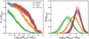 |
Fig. 6 Dust mass distributions of the IMTTs, Herbig disks (Stapper et al. 2022), disks in Lupus (Ansdell et al. 2016), and disks in Upper Sco (Barenfeld et al. 2016). The left panel shows the cumulative distributions, with the shaded region indicating the 1σ confidence interval. The right panel presents the probability distributions obtained by fitting a log-normal distribution to the cumulative distributions using a bootstrapping method. This figure shows a clear similarity between the IMTT and Herbig dust mass distributions. |
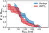 |
Fig. 7 Cumulative distributions of the 90% dust radii of the Herbig disks (S24) and of the IMTTs. Both samples have a similar radius distribution. |
5 Discussion
5.1 Evolution of Herbig disks
As IMTTs are the precursors of Herbig stars, the fact that the disk dust radii and masses are the same may come as a surprise at first, as we would typically expect an evolution toward smaller less massive disks due to dust evolutionary processes. As proposed in S22, the stopping of radial drift due to massive exoplanets can explain the large difference seen in the mass and size of Herbig disks when compared to T Tauri disks. As no difference in the radius or the dust mass is found between the Herbig disks and the IMTT disks, this may indicate that massive exoplanets have already formed in the IMTT disks stopping radial drift, resulting in a higher inferred disk mass. As both the radii and dust mass distributions are indistinguishable for both IMTTs and Herbigs, this implies that planets are forming early in their lifetime, dominating the (dust) evolution of these disks and giving very similar results. Furthermore, by selecting stars with infrared excess with masses between 1.5 and 3.5 solar masses within 300 pc, Iglesias et al. (2023) found that most of these pre-main sequence intermediate-mass stars are already evolved toward the debris disk stage in less than 10 Myr (though the lack of accretion in these stars may indicate that these disks are older). Given the stark similarities between Herbig and IMTT disks, this separation into full disks and debris disks should happen early on in the disk lifetime, and might highly depend on planet formation happening in these disks. Therefore, an important step forward would be to obtain a sample of even younger intermediate mass stars, possibly even earlier classes.
In S22, a dust mass dichotomy was found between the group I and group II disks as defined by Meeus et al. (2001). These are defined as the SED of group I disks can be reproduced by a power-law and a black-body, while the SED of group II disks can be reconstructed with a power-law alone. In particular the distribution of dust masses of the group II disks was very similar to the dust mass distribution of the disks in Lupus (Ansdell et al. 2016). On the other hand, the group I disks were more massive. Moreover, in contrast to the mostly full disks of the group II disks, group I disks were found to have large inner cavities. As Valegård et al. (2021) has classified the IMTTs into group I and group II based on the Meeus et al. (2001) classification, we are able ascertain whether the same differences between the two groups can be found.
Figure 11 presents the two cumulative mass distributions in the left panel, with the fitted log-normal probability distributions in the right panel. The results from this fit can be found in Table 3. We did not find a clear difference between the two populations, which was found for the Herbig disks (S22). However, we do note that the maximum and minimum dust masses are indeed lower for the group II disks compared to the group I disks. Comparing the distributions in the left panel of Fig. 11 with the distributions presented by S22, the mean dust mass of the group I disks is the same, the main difference is in the group II disks.
As noted by Honda et al. (2012), Maaskant et al. (2013), and S22, group I disks tend to be transitional disks, having large inner cavities, while group II disks tend to have full disks. With the IMTTs this is the case as well. For the resolved disks, the group I disks indeed show cavities (AK Sco, SR 21, HD 135344B, HD 142527, LkHα 330, and UX Tau), and the group II disks indeed have full disks (CR Cha, GW Ori, HD 142666, HT Lup, and RY Tau). We note that the classification of AK Sco by Valegård et al. (2021) is group I, while it is classified as group II by Guzmán-Díaz et al. (2021) as used by S22. Hence, the ALMA observations are of particular necessity to characterize the disk. The difference in mass and morphology between the group I and group II disks was interpreted by S22 as the group I disks forming massive exoplanets which create an inner cavity by stopping radial drift, while the group II disks most of the solid mass drifts inwards reducing the total inferred disk mass. As there is no difference in the inferred dust mass for the group I disks, when comparing the Herbig disks with the IMTT disks, no further evolution has happened in these particular disks, which is expected if the radial drift has stopped. On the other hand, the group II Herbig disks have lower disk masses than the group II IMTT disks, which is expected if the radial drift has not been stopped in the disk. So, most disks around intermediate-mass pre-main sequence stars converge quickly (i.e., within the timescale of the ages of the IMTT and Herbig disks) to small and compact disks unless prevented by a massive exoplanet. This should occur well before the age of the IMTT disks; namely, 5 Myr. We are mainly tracing the survivors of this process, as a large fraction of the pre-main sequence intermediate-mass stars are like those of Iglesias et al. (2023), without a disk, or the intermediate-mass equivalent of the Naked T Tauri stars. A key question to consider is whether this apparent quick convergence toward small, or absent, disks around pre-main sequence intermediate-mass stars is a natural phenomenon or related to biases ingrained in how these stellar populations are defined and/or observed. This on-off behavior has not been observed in T Tauri disks, where there is a clear decrease in dust mass over time (Drążkowska et al. 2023). This might be related to the need for high accretion rates to be classified as a Herbig star, as discussed in Grant et al. (2023). Moreover, the addition of mostly observing the brightest disks may bias this even further. A complete volume-limited millimeter survey of pre-main sequence intermediate-mass stars is therefore highly needed (Stapper et al., in prep.).
This hypothesis is also supported by observations of metallicities of the Herbig stars themselves (Kama et al. 2015; Guzmán-Díaz et al. 2023). Stars with a group I disk generally have lower metallicities compared to the group II disks, which is associated with the presence of massive exoplanets accreting the refractory elements and stopping the radial drift of the dust inwards. Brittain et al. (2023) pointed out that there is evidence that the opacities and temperatures of the dust are not the same for the two groups (Woitke et al. 2019). Group I disks tend to have smaller grains compared to group II disks, resulting in a higher inferred disk mass in the former compared to the latter. The fact that no differences among the group I and group II disks have been found (see Fig. 11) might be an indication that there are similar dust populations in the younger IMTT disks, which changes during the evolution toward a Herbig disk. This must be further investigated using longer wavelength observations.
Lastly, a recent work by Vioque et al. (2023) has shown that intermediate-mass young stellar objects become significantly less clustered with time. Hence, the IMTT disks are expected to be more clustered than Herbig stars. The fact that we do not find significant differences between both populations might indicate that the environment does not play a major role in the evolution of disks around intermediate-mass stars. Thus, study dedicated to the effect of the environment is needed to shed light on this issue.
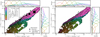 |
Fig. 8 13CO and C18O disk integrated luminosities for transitions J =2 − 1 (left panel) and J = 3 − 2 (right panel). The colors correspond to the DALI models from S24, while the black markers correspond to the observations. The vertical line in the left panel indicates the 13CO luminosity of SU Aur, as no C18O observations are available. |
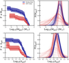 |
Fig. 9 Resulting gas masses obtained from the models of S24 are shown in the top row. The Herbig disks are shown in blue, while the distribution of the IMTT disks is shown in red. Combining the gas distributions with the dust mass distributions in Fig. 6 gives the gas-to-dust ratio distributions shown in the bottom row. |
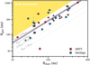 |
Fig. 10 Dust and gas 90% radii of the IMTT disks (red) and Herbig disks (blue). The fitted relation between the two parameters is shown as the solid lines. The relationship is the same for both Herbig and IMTT disks. In yellow the region is shown where the difference between the dust and gas radii cannot be explained by optical depth effects only (Trapman et al. 2019). The dashed black line is a fit through the IMTT disks excluding SR 21, GW Ori, HT Lup, and SU Aur, as these have extended emission beyond the disk. |
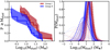 |
Fig. 11 Dust cumulative distributions of the group I and group II disks. There is no significant difference, in contrast to what is found for the Herbig disks (S22). The dotted distributions in the right panel are the dust mass distributions for the Herbig disks from S22. |
5.2 Planet formation around intermediate-mass stars
The dust masses of planet-forming disks have been directly compared to the solid mass of massive exoplanets in planetary systems by Tychoniec et al. (2020). They found a clear discrepancy between class II disks and the masses present in massive exoplanets, which would not be able to form. Even when taking into account observational biases this discrepancy would only not be a problem when the formation efficiency would be 100% (Mulders et al. 2021), which is likely not the case (see for an overview Drążkowska et al. 2023). As this comparison only has been done based on the dust mass inferred from continuum observations, this section also directly compares the exoplanetary masses to the gas masses we found in the disks around intermediate-mass stars. Moreover, we also include observational biases into the distribution.
To obtain an updated exoplanet mass distribution, we use the NASA exoplanet archive3, and select all confirmed exoplanets. Following Tychoniec et al. (2020), we set no detection method and use both the planet mass Mp and minimum planet mass Mp sin(i) in our distribution. To obtain a distribution for the intermediate-mass stars, we only include the planets around stars with a minimum mass of 1.5 M⊙. To obtain a distribution taking the observational biases into account, we use the work of Wolthoff et al. (2022), who determined giant exoplanet occurrence rates around stars with masses higher than 0.8 M⊙. Based on this work, we normalize the distribution to 1.3% for planetary masses higher than 9 Mjup, to 5.7% for masses higher than 2.7 Mjup and to 15.8% for the complete distribution. We note that planets with a period ranging from 80 to 3600 days are used here, so there are differences in the scales traced by planets and disks. Following Tychoniec et al. (2020), we know the total planetary mass includes both the core mass and the atmosphere, so we used the relationship from Thorngren et al. (2016) to obtain a heavy-element mass of the planet and we assume that this is the dust mass necessary to form the planet. The total gas (atmosphere) mass is then simply the difference between the planetary mass and the heavy-element mass of the planet. After the core and atmosphere masses, all planetary systems belonging to the same star are combined into a single mass. The number of stars hosting at least one giant planet is 10.7% (Wolthoff et al. 2022); hence, we can once again normalize the distribution so that it adds up to 10.7%. The resulting distribution is shown in Fig. 12.
Figure 12 also shows the dust mass and gas mass distributions after combining the data of our work with the dust masses from S22 and the gas masses from S24, after removing the duplicate disks from the sample of our work. The tail end of dust mass distribution of the disks is similar to the dust masses necessary to build the exoplanetary systems. However, an efficiency of 100% is necessary. This is in line with what was reported by Mulders et al. (2021). Comparing the exoplanet dust mass distribution with the disk gas mass distribution, assuming a gas-to-dust ratio of 100, the lower mass planets may be less of a problem to still form. Still, it is clear that the cores of the massive exoplanets should already have formed in these systems. This is in line with the previous discussion, as these exoplanets are thought to have a big impact on the evolution of disks around intermediate-mass stars.
Comparing the gas mass distributions, there still is more than enough gas mass available in the disks to form the exoplanet atmosphere. For a large fraction of the population, there is at least one or two orders of magnitude in difference with respect to the mass available in the disks, compared to the mass that is necessary to form the exoplanets. Hence, planet envelope accretion might still be ongoing, whereas the cores of the planets have already formed.
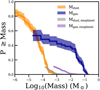 |
Fig. 12 Comparing the dust and gas mass cumulative distributions of the disks around intermediate mass (IMTT disks + Herbig disks) with a dust and gas mass distribution of exoplanets. |
6 Conclusion
In this work, we analyze the continuum, 12CO, 13CO, and C18O emission of 35 intermediate-mass T Tauri (IMTT) disks, all of them taken from ALMA archival data. The obtained dust masses and radii are compared to those of Herbig disks (Stapper et al. 2022), and T Tauri disks (Barenfeld et al. 2016; Ansdell et al. 2016). From our results, the following can be concluded:
IMTT disks have both the same dust mass distribution, assuming optically thin emission, and dust radius distribution as Herbig disks. Hence, a similar difference in dust mass is found when compared to the T Tauri disks;
The gas mass of IMTT disks, as determined with DALI thermochemical models, is possibly slightly lower than that of Herbig disks. This is likely due to the lack in sensitivity of the available CO isotopologue observations in the archive to obtain meaningful gas mass limits. Deeper observations of IMTT disks are urgently needed;
The gas radii are the same as that of the Herbig disks. Compared to the dust radii, the same ratio between the two is found as for the Herbig disks;
Dividing the IMTT disks into group I (rising FIR slope) and group II (decreasing FIR slope) disks reveals no significant difference regarding the dust mass. This is in stark contrast to what is found for Herbig disks, for which the inferred dust mass in the group II disks is lower than for the group I disks. This difference between the Herbig group I and group II disks might be indicative of different evolutionary scenarios happening in these two groups. Group I disks stay the same due to a massive exoplanet stopping radial drift, while the group II disks rapidly shrink over time due to radial drift decreasing the inferred disk mass;
As the mass and sizes of IMTT disks are the same as for Herbig disks, planet formation has likely already started in these disks, shaping their formation and subsequent evolution toward Herbig disks. Most disks around intermediate-mass pre-main sequence stars converge quickly to small disks unless prevented by a massive exoplanet. We are mainly tracing the survivors of this process, as most pre-main sequence intermediate mass stars are debris disks;
Comparing the disk dust mass distributions to the amount of dust mass in massive exoplanets, assuming that this equals the heavy-element mass of the planet, it is clear that the cores of the exoplanets already need to have formed, as there is not enough dust mass present in the disks. However, comparing the disk gas mass distributions to the mass in planetary envelopes, there is more than an order of magnitude in difference. This indicates that while the core of the exoplanets may already have formed, they are likely still accreting their envelope.
IMTTs are an important class of objects for understanding planet formation. This area of study would further benefit from targeted, high-resolution, deep-imaging observations with ALMA.
Acknowledgements
The research of LMS is supported by the Netherlands Research School for Astronomy (NOVA). The project leading to this publication has received support from ORP, that is funded by the European Union’s Horizon 2020 research and innovation programme under grant agreement No 101004719 [ORP]. This paper makes use of the following ALMA data: ADS/JAO.ALMA#2012.1.00158.S, #2012.1.00313.S, #2012.1.00870.S, #2013.1.00426.S, #2013.1.00437.S, #2013.1.00498.S, #2013.1.01075.S, #2015.1.00222.S, #2015.1.01353.S, #2015.1.01600.S, #2016.1.00204.S, #2016.1.00484.L, #2016.1.00545.S, #2016.1.01164.S, #2016.1.01338.S, #2017.1.00286.S, #2017.1.01353.S, #2017.1.01460.S, #2018.1.00689.S, #2018.1.01302.S, #2019.1.00703.S, #2019.1.00951.S, #2019.1.01813.S, #2021.2.00005.S, #2021.1.00854.S, #2021.1.01705.S, #2022.1.01155.S, #2022.1.01460.S. ALMA is a partnership of ESO (representing its member states), NSF (USA) and NINS (Japan), together with NRC (Canada), MOST and ASIAA (Taiwan), and KASI (Republic of Korea), in cooperation with the Republic of Chile. The Joint ALMA Observatory is operated by ESO, AUI/NRAO and NAOJ. This research has made use of the NASA Exoplanet Archive, which is operated by the California Institute of Technology, under contract with the National Aeronautics and Space Administration under the Exoplanet Exploration Program. We would like to thank Allegro for their support and computing resources for reducing and imaging the ALMA data. Also, we would like to thank Gijs Mulders for his useful comments on the exoplanet mass distribution. We also thank the referee for their careful consideration of our work and for their thoughtful comments which improved the manuscript. This work makes use of the following software: The Common Astronomy Software Applications (CASA) package (McMullin et al. 2007), Dust And LInes (DALI, Bruderer et al. 2012; Bruderer 2013), Python version 3.9, astropy (Astropy Collaboration 2013, 2018), lifelines (Davidson-Pilon et al. 2021), matplotlib (Hunter 2007), numpy (Harris et al. 2020), scipy (Virtanen et al. 2020) and seaborn (Waskom 2021).
Appendix A Additional tables
Source parameters used to calculate the dust masses, used for Keplerian masking, and the obtained dust and gas radii.
Continuum and CO line (J = 2 − 1 or J = 3 − 2) fluxes as well as dust and gas radii.
Appendix B Datasets used
In Table B.1 the project codes of the used datasets are listed together with their spatial and velocity resolution and the (line- free) rms noise.
Datasets and corresponding parameters for each IMTT disk. The rms noise is for an empty channel at the given velocity resolution with units mJy beam−1.
References
- ALMA Partnership, Brogan, C. L., Perez, L. M., et al. 2015, ApJ, 808, L3 [NASA ADS] [CrossRef] [Google Scholar]
- Andrews, S. M. 2020, ARA&A 58, 483 [Google Scholar]
- Andrews, S. M., Rosenfeld, K. A., Kraus, A. L., & Wilner, D. J. 2013, ApJ 771, 129 [Google Scholar]
- Ansdell, M., Williams, J. P., van der Marel, N., et al. 2016, ApJ, 828, 46 [Google Scholar]
- Ansdell, M., Williams, J. P., Manara, C. F., et al. 2017, AJ, 153, 240 [Google Scholar]
- Astropy Collaboration (Robitaille, T. P., et al.) 2013, A&A, 558, A33 [NASA ADS] [CrossRef] [EDP Sciences] [Google Scholar]
- Astropy Collaboration (Price-Whelan, A. M., et al.) 2018, AJ, 156, 123 [Google Scholar]
- Barenfeld, S. A., Carpenter, J. M., Ricci, L., & Isella, A. 2016, ApJ 827, 142 [Google Scholar]
- Beckwith, S. V. W., Sargent, A. I., Chini, R. S., & Guesten, R. 1990, AJ 99, 924 [Google Scholar]
- Bi, J., van der Marel, N., Dong, R., et al. 2020, ApJ, 895, L18 [Google Scholar]
- Booth, A. S., Ilee, J. D., Walsh, C., et al. 2023, A&A, 669, A53 [Google Scholar]
- Bosman, A. D., Walsh, C., & van Dishoeck, E. F. 2018, A&A 618, A182 [NASA ADS] [CrossRef] [EDP Sciences] [Google Scholar]
- Brittain, S. D., Kamp, I., Meeus, G., Oudmaijer, R. D., & Waters, L. B. F. M. 2023, Space Sci. Rev. 219, 7 [NASA ADS] [CrossRef] [Google Scholar]
- Brown, J. M., Blake, G. A., Qi, C., Dullemond, C. P., & Wilner, D. J. 2008, ApJ 675, L109 [NASA ADS] [CrossRef] [Google Scholar]
- Bruderer, S. 2013, A&A 559, A46 [NASA ADS] [CrossRef] [EDP Sciences] [Google Scholar]
- Bruderer, S., van Dishoeck, E. F., Doty, S. D., & Herczeg, G. J. 2012, A&A 541, A91 [NASA ADS] [CrossRef] [EDP Sciences] [Google Scholar]
- Calvet, N., Muzerolle, J., Briceño, C., et al. 2004, AJ, 128, 1294 [NASA ADS] [CrossRef] [Google Scholar]
- Cazzoletti, P., Manara, C. F., Baobab Liu, H., et al. 2019, A&A, 626, A11 [NASA ADS] [CrossRef] [EDP Sciences] [Google Scholar]
- Chauvin, G., Desidera, S., Lagrange, A. M., et al. 2017, A&A, 605, L9 [NASA ADS] [CrossRef] [EDP Sciences] [Google Scholar]
- Czekala, I., Andrews, S. M., Jensen, E. L. N., et al. 2015, ApJ, 806, 154 [Google Scholar]
- Daemgen, S., Petr-Gotzens, M. G., Correia, S., et al. 2013, A&A, 554, A43 [NASA ADS] [CrossRef] [EDP Sciences] [Google Scholar]
- Davidson-Pilon, C., Kalderstam, J., Jacobson, N., et al. 2021, https://doi.org/10.5281/zenodo.4579431 [Google Scholar]
- Drążkowska, J., & Dullemond, C. P. 2018, A&A 614, A62 [NASA ADS] [CrossRef] [EDP Sciences] [Google Scholar]
- Drążkowska, J., Bitsch, B., Lambrechts, M., et al. 2023, in Astronomical Society of the Pacific Conference Series, 534, Protostars and Planets VII, eds. S. Inutsuka, Y. Aikawa, T. Muto, K. Tomida, & M. Tamura, 717 [Google Scholar]
- Fedele, D., Carney, M., Hogerheijde, M. R., et al. 2017, A&A, 600, A72 [NASA ADS] [CrossRef] [EDP Sciences] [Google Scholar]
- Francis, L., & van der Marel, N. 2020, ApJ, 892, 111 [Google Scholar]
- Fulton, B. J., Rosenthal, L. J., Hirsch, L. A., et al. 2021, ApJS, 255, 14 [NASA ADS] [CrossRef] [Google Scholar]
- Garufi, A., Ginski, C., van Holstein, R. G., et al. 2024, A&A, 685, A53 [NASA ADS] [CrossRef] [EDP Sciences] [Google Scholar]
- Ginski, C., Facchini, S., Huang, J., et al. 2021, ApJ, 908, L25 [NASA ADS] [CrossRef] [Google Scholar]
- Ginski, C., Garufi, A., Benisty, M., et al. 2024, A&A, 685, A52 [NASA ADS] [CrossRef] [EDP Sciences] [Google Scholar]
- Grant, S. L., Stapper, L. M., Hogerheijde, M. R., et al. 2023, AJ, 166, 147 [NASA ADS] [CrossRef] [Google Scholar]
- Guzmán-Díaz, J., Mendigutía, I., Montesinos, B., et al. 2021, A&A, 650, A182 [NASA ADS] [CrossRef] [EDP Sciences] [Google Scholar]
- Guzmán-Díaz, J., Montesinos, B., Mendigutía, I., et al. 2023, A&A, 671, A140 [NASA ADS] [CrossRef] [EDP Sciences] [Google Scholar]
- Harris, C. R., Millman, K. J., van der Walt, S. J., et al. 2020, Nature, 585, 357 [NASA ADS] [CrossRef] [Google Scholar]
- Hartmann, L., Calvet, N., Gullbring, E., & D’Alessio, P. 1998, ApJ, 495, 385 [Google Scholar]
- Herbig, G. H. 1960, ApJS 4, 337 [Google Scholar]
- Herbig, G. H. 1977, ApJ 214, 747 [Google Scholar]
- Hildebrand, R. H. 1983, QJRAS 24, 267 [NASA ADS] [Google Scholar]
- Honda, M., Maaskant, K., Okamoto, Y. K., et al. 2012, ApJ, 752, 143 [Google Scholar]
- Houk, N. 1978, Michigan catalogue of two-dimensional spectral types for the HD stars (Ann Arbor : Dept. of Astronomy, University of Michigan: distributed by University Microfilms International) [Google Scholar]
- Houk, N. 1982, Michigan Catalogue of Two-dimensional Spectral Types for the HD stars. 3. Declinations -40_f0 to -26_f0 (Ann Arbor : Dept. of Astronomy, University of Michigan : distributed by University Microfilms International) [Google Scholar]
- Houk, N., & Swift, C. 1999, Michigan Spectral Survey 5, 0 [Google Scholar]
- Huang, J., Andrews, S. M., Dullemond, C. P., et al. 2018, ApJ, 869, L42 [NASA ADS] [CrossRef] [Google Scholar]
- Hunter, J. D. 2007, Comput. Sci. Eng. 9, 90 [NASA ADS] [CrossRef] [Google Scholar]
- Iglesias, D. P., Panic, O., van den Ancker, M., et al. 2023, MNRAS, 519, 3958 [Google Scholar]
- Izquierdo, A. F., Testi, L., Facchini, S., et al. 2023, A&A, 674, A113 [NASA ADS] [CrossRef] [EDP Sciences] [Google Scholar]
- Johnson, J. A., Butler, R. P., Marcy, G. W., et al. 2007, ApJ, 670, 833 [Google Scholar]
- Johnson, J. A., Aller, K. M., Howard, A. W., & Crepp, J. R. 2010, PASP 122, 905 [Google Scholar]
- Kama, M., Folsom, C. P., & Pinilla, P. 2015, A&A 582, L10 [NASA ADS] [CrossRef] [EDP Sciences] [Google Scholar]
- Kataoka, A., Tsukagoshi, T., Momose, M., et al. 2016, ApJ, 831, L12 [Google Scholar]
- Kim, S., Takahashi, S., Nomura, H., et al. 2020, ApJ, 888, 72 [Google Scholar]
- Köhler, R., Kasper, M., Herbst, T. M., Ratzka, T., & Bertrang, G. H. M. 2016, A&A 587, A35 [NASA ADS] [CrossRef] [EDP Sciences] [Google Scholar]
- Kurtovic, N. T., Pérez, L. M., Benisty, M., et al. 2018, ApJ, 869, L44 [Google Scholar]
- Lagrange, A. M., Bonnefoy, M., Chauvin, G., et al. 2010, Science, 329, 57 [Google Scholar]
- Liu, Y., Linz, H., Fang, M., et al. 2022, A&A, 668, A175 [NASA ADS] [CrossRef] [EDP Sciences] [Google Scholar]
- Long, F., Pinilla, P., Herczeg, G. J., et al. 2018, ApJ, 869, 17 [Google Scholar]
- Lynden-Bell, D., & Pringle, J. E. 1974, MNRAS 168, 603 [Google Scholar]
- Maaskant, K. M., Honda, M., Waters, L. B. F. M., et al. 2013, A&A, 555, A64 [NASA ADS] [CrossRef] [EDP Sciences] [Google Scholar]
- Manara, C. F., Morbidelli, A., & Guillot, T. 2018, A&A 618, L3 [NASA ADS] [CrossRef] [EDP Sciences] [Google Scholar]
- Manara, C. F., Ansdell, M., Rosotti, G. P., et al. 2023, in Astronomical Society of the Pacific Conference Series, 534, Protostars and Planets VII, eds. S. Inutsuka, Y. Aikawa, T. Muto, K. Tomida, & M. Tamura, 539 [NASA ADS] [Google Scholar]
- Manoj, P., Bhatt, H. C., Maheswar, G., & Muneer, S. 2006, ApJ 653, 657 [Google Scholar]
- Marigo, P., Girardi, L., Bressan, A., et al. 2017, ApJ, 835, 77 [Google Scholar]
- Marois, C., Macintosh, B., Barman, T., et al. 2008, Science, 322, 1348 [Google Scholar]
- Marois, C., Zuckerman, B., Konopacky, Q. M., Macintosh, B., & Barman, T. 2010, Nature 468, 1080 [NASA ADS] [CrossRef] [Google Scholar]
- McMullin, J. P., Waters, B., Schiebel, D., Young, W., & Golap, K. 2007, in Astronomical Society of the Pacific Conference Series, 376, Astronomical Data Analysis Software and Systems XVI, eds. R. A. Shaw, F. Hill, & D. J. Bell, 127 [NASA ADS] [Google Scholar]
- Meeus, G., Waters, L. B. F. M., Bouwman, J., et al. 2001, A&A, 365, 476 [CrossRef] [EDP Sciences] [Google Scholar]
- Miotello, A., Bruderer, S., & van Dishoeck, E. F. 2014, A&A 572, A96 [NASA ADS] [CrossRef] [EDP Sciences] [Google Scholar]
- Miotello, A., van Dishoeck, E. F., Kama, M., & Bruderer, S. 2016, A&A 594, A85 [NASA ADS] [CrossRef] [EDP Sciences] [Google Scholar]
- Miotello, A., Kamp, I., Birnstiel, T., Cleeves, L. C., & Kataoka, A. 2023, in Astronomical Society of the Pacific Conference Series, 534, Protostars and Planets VII, eds. S. Inutsuka, Y. Aikawa, T. Muto, K. Tomida, & M. Tamura, 501 [NASA ADS] [Google Scholar]
- Mora, A., Merín, B., Solano, E., et al. 2001, A&A, 378, 116 [NASA ADS] [CrossRef] [EDP Sciences] [Google Scholar]
- Mulders, G. D., Pascucci, I., Ciesla, F. J., & Fernandes, R. B. 2021, ApJ 920, 66 [NASA ADS] [CrossRef] [Google Scholar]
- Nielsen, E. L., De Rosa, R. J., Macintosh, B., et al. 2019, AJ, 158, 13 [Google Scholar]
- Öberg, K. I., Guzmán, V. V., Walsh, C., et al. 2021, ApJS, 257, 1 [CrossRef] [Google Scholar]
- Ohashi, N., Tobin, J. J., Jørgensen, J. K., et al. 2023, ApJ, 951, 8 [NASA ADS] [CrossRef] [Google Scholar]
- Pérez, L. M., Isella, A., Carpenter, J. M., & Chandler, C. J. 2014, ApJ 783, L13 [Google Scholar]
- Pinilla, P., Benisty, M., Kurtovic, N. T., et al. 2022, A&A, 665, A128 [NASA ADS] [CrossRef] [EDP Sciences] [Google Scholar]
- Pinte, C., Price, D. J., Ménard, F., et al. 2018, ApJ, 860, L13 [Google Scholar]
- Reipurth, B., Herbig, G., & Aspin, C. 2010, AJ 139, 1668 [Google Scholar]
- Rota, A. A., Manara, C. F., Miotello, A., et al. 2022, A&A, 662, A121 [NASA ADS] [CrossRef] [EDP Sciences] [Google Scholar]
- Rydgren, A. E., & Vrba, F. J. 1984, AJ 89, 399 [NASA ADS] [CrossRef] [Google Scholar]
- Savvidou, S., & Bitsch, B. 2025, A&A, 693, A302 [NASA ADS] [Google Scholar]
- Segura-Cox, D. M., Schmiedeke, A., Pineda, J. E., et al. 2020, Nature, 586, 228 [NASA ADS] [CrossRef] [Google Scholar]
- Stapper, L. M., Hogerheijde, M. R., van Dishoeck, E. F., & Mentel, R. 2022, A&A 658, A112 [NASA ADS] [CrossRef] [EDP Sciences] [Google Scholar]
- Stapper, L. M., Hogerheijde, M. R., van Dishoeck, E. F., et al. 2024, A&A, 682, A149 [NASA ADS] [CrossRef] [EDP Sciences] [Google Scholar]
- Suárez, O., García-Lario, P., Manchado, A., et al. 2006, A&A, 458, 173 [NASA ADS] [CrossRef] [EDP Sciences] [Google Scholar]
- Teague, R., Bae, J., Bergin, E. A., Birnstiel, T., & Foreman-Mackey, D. 2018, ApJ 860, L12 [NASA ADS] [CrossRef] [Google Scholar]
- Temmink, M., Booth, A. S., van der Marel, N., & van Dishoeck, E. F. 2023, A&A, 675, A131 [NASA ADS] [CrossRef] [EDP Sciences] [Google Scholar]
- Thorngren, D. P., Fortney, J. J., Murray-Clay, R. A., & Lopez, E. D. 2016, ApJ 831, 64 [NASA ADS] [CrossRef] [Google Scholar]
- Torres, C. A. O., Quast, G. R., da Silva, L., et al. 2006, A&A, 460, 695 [NASA ADS] [CrossRef] [EDP Sciences] [Google Scholar]
- Trapman, L., Facchini, S., Hogerheijde, M. R., van Dishoeck, E. F., & Bruderer, S. 2019, A&A 629, A79 [NASA ADS] [CrossRef] [EDP Sciences] [Google Scholar]
- Tychoniec, L., Manara, C. F., Rosotti, G. P., et al. 2020, A&A, 640, A19 [NASA ADS] [CrossRef] [EDP Sciences] [Google Scholar]
- Valegård, P. G., Waters, L. B. F. M., & Dominik, C. 2021, A&A 652, A133 [NASA ADS] [CrossRef] [EDP Sciences] [Google Scholar]
- Valegård, P. G., Ginski, C., Derkink, A., et al. 2024, A&A, 685, A54 [NASA ADS] [CrossRef] [EDP Sciences] [Google Scholar]
- van der Marel, N., & Mulders, G. D. 2021, AJ, 162, 28 [NASA ADS] [CrossRef] [Google Scholar]
- van der Marel, N., van Dishoeck, E. F., Bruderer, S., Pérez, L., & Isella, A. 2015, A&A, 579, A106 [NASA ADS] [CrossRef] [EDP Sciences] [Google Scholar]
- van Terwisga, S. E., van Dishoeck, E. F., Mann, R. K., et al. 2020, A&A, 640, A27 [NASA ADS] [CrossRef] [EDP Sciences] [Google Scholar]
- van Terwisga, S. E., Hacar, A., van Dishoeck, E. F., Oonk, R., & Portegies Zwart, S. 2022, A&A 661, A53 [NASA ADS] [CrossRef] [EDP Sciences] [Google Scholar]
- Vioque, M., Oudmaijer, R. D., Baines, D., Mendigutía, I., & Pérez-Martínez, R. 2018, A&A 620, A128 [NASA ADS] [CrossRef] [EDP Sciences] [Google Scholar]
- Vioque, M., Oudmaijer, R. D., Schreiner, M., et al. 2020, A&A, 638, A21 [NASA ADS] [CrossRef] [EDP Sciences] [Google Scholar]
- Vioque, M., Oudmaijer, R. D., Wichittanakom, C., et al. 2022, ApJ, 930, 39 [NASA ADS] [CrossRef] [Google Scholar]
- Vioque, M., Cavieres, M., Pantaleoni González, M., et al. 2023, AJ, 166, 183 [NASA ADS] [CrossRef] [Google Scholar]
- Virtanen, P., Gommers, R., Oliphant, T. E., et al. 2020, Nature Methods, 17, 261 [CrossRef] [Google Scholar]
- Waskom, M. L. 2021, J. Open Source Softw. 6, 3021 [CrossRef] [Google Scholar]
- Wichittanakom, C., Oudmaijer, R. D., Fairlamb, J. R., et al. 2020, MNRAS, 493, 234 [Google Scholar]
- Woitke, P., Kamp, I., Antonellini, S., et al. 2019, PASP, 131, 064301 [NASA ADS] [CrossRef] [Google Scholar]
- Wolthoff, V., Reffert, S., Quirrenbach, A., et al. 2022, A&A, 661, A63 [NASA ADS] [CrossRef] [EDP Sciences] [Google Scholar]
- Xin, Z., Espaillat, C. C., Rilinger, A. M., Ribas, Á., & Macías, E. 2023, ApJ 942, 4 [NASA ADS] [CrossRef] [Google Scholar]
BH Cep, BO Cep, HD 200775, SV Cep, XY Per.
All Tables
Source parameters used to calculate the dust masses, used for Keplerian masking, and the obtained dust and gas radii.
Continuum and CO line (J = 2 − 1 or J = 3 − 2) fluxes as well as dust and gas radii.
Datasets and corresponding parameters for each IMTT disk. The rms noise is for an empty channel at the given velocity resolution with units mJy beam−1.
All Figures
|
Fig. 1 HR-diagram of the Herbig star sample of S22, and the compiled IMTT sample in this work. The effective temperatures and luminosities are taken from Vioque et al. (2018) and Valegård et al. (2021) for the Herbig stars and IMTT stars, respectively. Pre-main sequence tracks of different intermediate-mass stars and an isochrone of 2.5 Myr as the dashed line are taken from Marigo et al. (2017). |
| In the text | |
|
Fig. 2 Histogram of the spectral types (left panel) and stellar masses (right panel) of the IMTTs in this work (from Valegård et al. 2021) compared to the Herbig star sample of S22 and references therein, as well as the surveys of Lupus (Ansdell et al. 2016) and Upper Sco (Barenfeld et al. 2016). |
| In the text | |
|
Fig. 3 Histogram of the disk integrated C18O luminosities of models run by the thermochemical code DALI for three different disk masses, as indicated in the top-left of each panel. A comparison is done between the models used by S24 (gray), and models for which the stellar effective temperature has been lowered to an IMTT appropriate value either with (red) or without (blue) accretion UV added. The lower effective temperature of the IMTT star increases the C18O luminosity for the lowest mass disks compared to the Herbig disk models, as there is less UV emission and therefore less photodissociation of CO. Adding the accretion UV increases the photodissociation of CO, moving the C18O luminosity back to Herbig disk levels. |
| In the text | |
|
Fig. 4 Continuum images of intermediate-mass T Tauri disks with a detection, using a sinh stretch. The size of the image is indicated by the bar of size 100 au on the bottom right of each panel with the corresponding angular size. The beam size is shown as the ellipse on the bottom left of each panel. The group classification can be found in Table A.1. |
| In the text | |
|
Fig. 5 12CO, 13CO, and C18O velocity integrated-intensity maps as obtained with Keplerian masking for all IMTTs which have a detection in at least one of the three isotopologues. An empty panel indicates that no observations are available of that particular isotopologue. |
| In the text | |
|
Fig. 6 Dust mass distributions of the IMTTs, Herbig disks (Stapper et al. 2022), disks in Lupus (Ansdell et al. 2016), and disks in Upper Sco (Barenfeld et al. 2016). The left panel shows the cumulative distributions, with the shaded region indicating the 1σ confidence interval. The right panel presents the probability distributions obtained by fitting a log-normal distribution to the cumulative distributions using a bootstrapping method. This figure shows a clear similarity between the IMTT and Herbig dust mass distributions. |
| In the text | |
|
Fig. 7 Cumulative distributions of the 90% dust radii of the Herbig disks (S24) and of the IMTTs. Both samples have a similar radius distribution. |
| In the text | |
|
Fig. 8 13CO and C18O disk integrated luminosities for transitions J =2 − 1 (left panel) and J = 3 − 2 (right panel). The colors correspond to the DALI models from S24, while the black markers correspond to the observations. The vertical line in the left panel indicates the 13CO luminosity of SU Aur, as no C18O observations are available. |
| In the text | |
|
Fig. 9 Resulting gas masses obtained from the models of S24 are shown in the top row. The Herbig disks are shown in blue, while the distribution of the IMTT disks is shown in red. Combining the gas distributions with the dust mass distributions in Fig. 6 gives the gas-to-dust ratio distributions shown in the bottom row. |
| In the text | |
|
Fig. 10 Dust and gas 90% radii of the IMTT disks (red) and Herbig disks (blue). The fitted relation between the two parameters is shown as the solid lines. The relationship is the same for both Herbig and IMTT disks. In yellow the region is shown where the difference between the dust and gas radii cannot be explained by optical depth effects only (Trapman et al. 2019). The dashed black line is a fit through the IMTT disks excluding SR 21, GW Ori, HT Lup, and SU Aur, as these have extended emission beyond the disk. |
| In the text | |
|
Fig. 11 Dust cumulative distributions of the group I and group II disks. There is no significant difference, in contrast to what is found for the Herbig disks (S22). The dotted distributions in the right panel are the dust mass distributions for the Herbig disks from S22. |
| In the text | |
|
Fig. 12 Comparing the dust and gas mass cumulative distributions of the disks around intermediate mass (IMTT disks + Herbig disks) with a dust and gas mass distribution of exoplanets. |
| In the text | |
Current usage metrics show cumulative count of Article Views (full-text article views including HTML views, PDF and ePub downloads, according to the available data) and Abstracts Views on Vision4Press platform.
Data correspond to usage on the plateform after 2015. The current usage metrics is available 48-96 hours after online publication and is updated daily on week days.
Initial download of the metrics may take a while.