| Issue |
A&A
Volume 693, January 2025
|
|
|---|---|---|
| Article Number | A66 | |
| Number of page(s) | 8 | |
| Section | Planets, planetary systems, and small bodies | |
| DOI | https://doi.org/10.1051/0004-6361/202348940 | |
| Published online | 03 January 2025 | |
Rotation periods of asteroids from light curves of TESS data
1
Université Côte d’Azur, Observatoire de la Côte d’Azur, CNRS, Laboratoire Lagrange,
06304
Nice Cedex 4,
France
2
Institute of Applied Astronomy, Russian Academy of Sciences,
Kutuzova emb. 10,
St. Petersburg,
Russia
★ Corresponding authors; This email address is being protected from spambots. You need JavaScript enabled to view it.
; This email address is being protected from spambots. You need JavaScript enabled to view it.
Received:
13
December
2023
Accepted:
18
March
2024
Abstract
Context. Understanding the dynamical evolution of asteroids through the secular Yarkovsky effect requires the determination of many physical properties, including the rotation period.
Aims. We propose a method aimed at obtaining a robust determination of the rotation period of asteroids, while avoiding the pitfalls of aliases. We applied this approach to thousands of asteroid light curves measured by the NASA TESS mission.
Methods. We developed a robust period-analysis algorithm based on a Fourier series. Our approach includes a comparison of the results from multiple orders and tests on the number of extremes to identify and reject potential aliases. We also provide the uncertainty interval for the result as well as additional periods that may be plausible.
Results. We report the rotation period for 4521 asteroids within a precision of 10%. A comparison with the literature (whenever available) reveals a very good agreement and validates the approach presented here. Our approach also highlights cases for which the determination of the period should be considered invalid. The dataset presented here confirms the apparent small number of asteroids with a rotation between 50 and 100 h and correlated with diameter. The amplitude of the light curves is found to increase toward smaller diameters, as asteroids become less and less spherical. Finally, there is a systematic difference between the broad C and S complex in the amplitude-period, revealing the statistically lower density of C-types compared to S-type asteroids.
Conclusions. Our approach to the determination of asteroid rotation period is based on simple concepts, yet it is nonetheless robust. It can be applied to large corpora of time series photometry, such as those extracted from exoplanet transit surveys.
Key words: methods: data analysis / astronomical databases: miscellaneous / minor planets, asteroids: general
© The Authors 2025
 Open Access article, published by EDP Sciences, under the terms of the Creative Commons Attribution License (https://creativecommons.org/licenses/by/4.0), which permits unrestricted use, distribution, and reproduction in any medium, provided the original work is properly cited.
This article is published in open access under the Subscribe to Open model. This email address is being protected from spambots. You need JavaScript enabled to view it. to support open access publication.
1 Introduction
The asteroids forming the Main Belt between Mars and Jupiter are remnants of the bricks that accreted to form the planets. Prints of the events that occurred in the early Solar System are still present in the distribution of their orbit, size, and composition (DeMeo & Carry 2014; Morbidelli et al. 2015; Clement et al. 2020). The current population, however, differs from its pristine distribution. Giga-years of collisions have fragmented bodies and created clumps of objects called families (Hirayama 1918; Zappala et al. 1990; Milani et al. 2014). All dynamical structures are furthermore secularly spreading through the non-gravitational Yarkovsky effect (Bottke et al. 2001).
The Yarkosky effect results from the delayed re-emission of the Solar incident flux and depends on many physical and surface properties such as diameter, albedo, density, obliquity, and rotation period (Vokrouhlický et al. 2015). Some properties, such as the diameter, are available for hundreds of thousands of asteroids thanks to mid-infrared (MIR) surveys such as IRAS, AKARI, or WISE (Tedesco et al. 2002; Usui et al. 2011; Masiero et al. 2011). Others, such as the density or thermal inertia, are much less constrained and available for only a tiny fraction of asteroids (see Berthier et al. 2023, for a recent compilation).
Spin properties (rotation period and coordinates) typically require numerous photometric measurements over a long period of time, covering several apparitions (Durech et al. 2015). These measurements can be dense-in-time time series, hereafter referred to as “light curves” (Kaasalainen et al. 2001), or they can be photometry sparse-in-time, collected by surveys (Kaasalainen 2004). However, owing to the potential multiple period aliases from sparse data, a light curve often helps to unambiguously determine the rotation period (Ďurech et al. 2015).
Surveys aimed at discovering and characterizing exoplanets via the transit method offer a tremendous amount of time series over wide fields in which asteroids can be searched for (Berthier et al. 2016; Grice et al. 2017). Recently, Pál et al. (2020) extracted light curves for 9912 Solar system objects (SSOs) from the Transiting Exoplanet Survey Satellite (TESS) first data release (DR1). The released catalog of asteroid light curves and periods is dubbed TSSYS-DR1. Pál et al. (2020) determined the rotation period of 9912 asteroids by fitting second order Fourier series. However, in some cases, such as asteroids (118) Peitho, (511) Davida, and (775) Lumiere among many others, it is not enough to describe accurately the light curve as second-order in the Fourier Series (Scheirich & Pravec 2009), leading to potentially erroneous period determinations.
In this work, we aim here to analyse the large sample of light curves released by Pál et al. (2020) with a robust perioddetermination algorithm. We present examples demonstrating that a Fourier series of the second order is often not sufficient to describe asteroid light curves. The article is organized as follows. In Sect. 2, we describe how we model the light curve of asteroids. In Sect. 3, we explain how we selected the optimum solution among different potentially degenerated solutions. We then present the results of the analysis of the TESS light curves in Sect. 4. We validate these results in Sect. 5 and we discuss their implications in Sect. 6. Finally, we give our conclusions in Sect. 7.
2 Modeling asteroid light curves
The apparent visual magnitude of an asteroid depends on the geometry of observation and can be described as (Bowell et al. 1989):
 (1)
(1)
where H is the absolute magnitude of the asteroid, r and Δ are the heliocentric distance and range to the observer (in au), g(t) is a periodic function related to the asteroid shape in rotation, and the phase function ϕ(α) describes how brightness evolves with the phase angle α (the Sun-asteroid-observer angle; see Bowell et al. 1989; Muinonen et al. 2010, for the different functions in usage in the community). The present study focuses on the determination of the period of the g(t) function.
2.1 Reduction to unit distances
To find the rotation period of an asteroid, we first take into account the change of visual magnitude occasioned by the changing distances due to the asteroid and Earth orbital motions. For each observation, i, we compute:
 (2)
(2)
which depends only on the asteroid absolute magnitude, rotation, and phase function. We also correct the timing of the i-th observation by:
 (3)
(3)
where c is the speed of light, t′ is the recorded observation epoch, and t is the actual epoch for the observed visual magnitude.
Before moving into further analysis, we exclude the observations deemed to be unreliable. We exclude all observations with flags different from 0 (see Table 1 in Pál et al. 2020, for a full description of the flags). Observations with flag values 128 and 16 384 (manual exclusion for anomaly or because outlier) were only excluded from the first iteration of fitting and may be included in the next iterations according to a 3σ rule.
2.2 Fourier fitting and phase function
The reduced V′ magnitude fluctuates because of the phase function ϕ(α) and the periodic function g(t), with a period equals to the asteroid’s synodic rotation period. The function g(t) is decomposed into a Fourier series:
 (4)
(4)
where f is the frequency of rotation (cycles per day), t is time (in days), k is the maximal number of Fourier series, and {Aj, Bj} the amplitude coefficients at each frequency. In the present analysis, we consider values of k up to k = 10.
The phase angles of asteroids observed by TESS typically span a small range or a few degrees only, around 3° of phase, with minimum values of typically 3° and maximum values around 8° (Fig. 1). The lack of coverage of the opposition surge implies that the system of equations is ill-conditioned for finding the parameters of the usual phase functions H, G (Bowell et al. 1989) or H, G1, G2 (Muinonen et al. 2010). We refer to Mahlke et al. (2021) for a discussion of phase coverage. We hence follow here the approach by Pál et al. (2020) of describing the phase function as a second-degree polynomial:

This approach precludes the determination of the absolute magnitude, H, of an asteroid, but that is not our goal. On the other hand, the fitting is accurate and well conditioned. We limit here the possible range of values for c1 and c2 to ascertain the physical results (i.e., increasing reduced magnitude with phase angle). We used the H, G phase function (Bowell et al. 1989) as a reference and assumed that the parameter G cannot take values outside the given range (−0.25, 0.95). The H-G function cannot be properly approximated by a second degree polynomial. That is why we find an approximation on the arc of 1°. For each angle α from {1°, 2°, 3°,…, 120°} we construct two phase curves with (Gmax = 0.95 and Gmin = −0.25). We then fit parameters c0, c1, and c2 on the arc (α − 0.5°, α + 0.5°). The maximal and minimal values for c1 and c2 found this way for a particular phase angle are then used as boundaries for the fit of TESS data. We should note here that the free term c0 encompasses H, which is removed from the fitting procedure.
For a given frequency, f , we found the parameters c0 , c1 , c2, {Aj, Bj}j=1,k via a least-squares minimisation. We took the weights of observations into account according to chapter VIII in Linnik (1961). We also excluded observations differing from the fit by more than 3σ iteratively until the procedure converged.
We put “soft” limitations on the parameters c1 and c2 in the least-squares fitting procedure, so that these values cannot be substantially outside the interval ![Mathematical equation: $\left[ {c_j^{\max },c_j^{\min }} \right]$](/articles/aa/full_html/2025/01/aa48940-23/aa48940-23-eq6.png) . We added the following two equations to the system of conditional equations (Gubanov 1997, p. 73):
. We added the following two equations to the system of conditional equations (Gubanov 1997, p. 73):
 (5)
(5)
where α is a minimal phase angle in the observation data of the asteroid. These equations are added with weights of  . The aim of it is to guide the fitting procedure toward mean values of c1 and c2 of
  , with standard deviations of
  . We present in Fig. 2 an example of the fitting procedure, on asteroid (3) Juno.
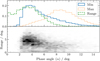 |
Fig. 1 Top: distribution of the maximal, minimal, and range of phase angles. Bottom: range of phase as a function of the minimum phase angle. |
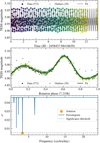 |
Fig. 2 Example of light curve fit for asteroid (3) Juno. Top: TSSYS-DR1 data as function of time. Observations are plotted as dots, color-coded by epoch. Crosses represent data rejected by the fitting procedure (see text). The line represents the best fit. Middle: same as above, folded over a rotation period ( |

3 Selection of the best model
To find the rotational period, we sampled different frequencies, f, and for each of them we fit via least-squares routine the 2k + 3 parameters c0 , c1 , c2, {Aj, Bj}j=1,k. We did not simply select the solution with the lowest residuals; rather, we imposed the following criteria to be fulfilled.
3.1 Defining the frequency range
First, at least two full periods of the asteroid rotation must have been observed. Shorter coverage could indeed result in spurious period determination. We thus set a minimal frequency:
 (6)
(6)
where tmax and tmin are the epochs of the last and first observation, respectively. Owing to the TESS observing strategy, each sector is observed for approximately a month, namely: fmin > 0.05 days−1.
Furthermore, TESS full-frame images are taken every 30 min approximately (Pál et al. 2020). The maximal possible frequency is thus analogous to a Nyquist-limit, adapted to the case of irregular sampling (Eyer & Bartholdi 1999): where p is the largest value, such that each ti can be written as ti = t0 + nip, for integers, ni; then the Nyquist frequency is  . AA direct citations not needed in AA. Of course, the equality ti = t0 + nip cannot be fulfilled precisely, so we allowed for a 2% accuracy for this equation. For most asteroids in TSSYS-DR1, the Nyquist frequency is approximately 24 days−1, implying a minimal rotational period of about 1 hour (however, in some cases,
  reached about 48 days−1). We set the right end of the frequency interval to 24 days−1, thus: a minimal rotation period of 1 hour.
We note that the maximal frequency decreases with the number of Fourier series (i.e., greater k). The k series contains a term in cos(2πfkt) which period is 1/kf, and hence the maximal frequency is fNy/k. We consider 40 001 possible frequencies on the interval between fmin and min(fNy,24) for k = 1. For k > 1, we keep the frequency steps and the interval becomes [fmin,min(fNy/k,24)].
3.2 Choosing the optimum fit
For each number of Fourier series, k, we first found the best fit according to our criteria (Eq. (7)). We then compared fits obtained with different k to select the final solution.
The main criterion is the minimal value of standard deviation of one observation σ, which is a classical unbiased estimate of a observational dispersion (Linnik 1961):
 (7)
(7)
where Oi and Ci are i-th observation and computed magnitude, pi is the weight of i-th observation (taken as  ), Nobs is the number of observations, Nincl is the number of observations included in the fit, and npar is the number of fitted parameters (2k + 3).
We note that the number of observations included in the fit can slightly differ for each frequency. The factor Nobs in Nobs /Σj pj is required to bring the value σ to the observational error with mean weight. This does not change the result but helps us understand the accuracy of the fit. We chose the model with the lowest value of σ as solution for this number of Fourier series.
If the shape of an asteroid is well-described by a tri-axial ellipsoid, the light-curve is expected to display two local maxima and two local minima. However, the number of local maxima from fitting can be up to k. For instance, eight local minima can appear with eight Fourier series. This point is critical as many objects present two solutions for the frequency, only differing by a factor of two. There are cases where the two solutions are in reality associated with the same period (e.g., Fig. 3), particularly if one of the solutions refers to a light curve with one local maxima only.
We repeated the above procedure for each number of Fourier series, k, from 1 to 10. For each k, we have a single candidate for the final model and final period. To choose among these, we used the F-test and computed it for each pair of models. The F- test tells us whether the difference between two dispersions is significant or not. The F-test gives us the probability (p-value) for the first model being better than the second one. In total, we obtained 10 × 9/2 = 45 results for the F-tests. Following the Occam’s razor rule, we chose the model with smallest possible number of Fourier series. We chose the smallest k for which no other model is significantly better, namely, such a k value that all the p-values of F-tests of k and any j are less than 95%.
For this chosen model, we computed its sigma-level (F- test, p-value 90%). With the F-test, we computed pvalue = Ftest(σ1 , σ2, n1, n2). However, we can also solve the reverse problem: for a given σ1, the aim is to find the σ2 of the second model, so that the p-value is 90%. In this case, we used the same number of used observations (n1 = n2). This is how we define the sigma-level. All the models with σ values lower than this threshold are also possible, with their associated rotation period. As a result, we provide a range of valid rotation period and, whenever applicable, all the other potential periods that are not in the computed interval (i.e., generally a multiple of 2 of the period). In the case of a high number of possible periods, we provide the whole interval for all, which means that the result is imprecise.
Also, we checked whether using a different number of Fourier series can lead to any plausible solutions (the σ value of which is lower than for the chosen one). In general, this is the case when for a higher order of Fourier series, the frequency can only be low (so the period is high) and the period is doubled or even tripled. These periods might be realistic (i.e., the σ is still lower than for chosen solution), but still unlikely.
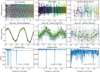 |
Fig. 3 Illustrations of the advantages of the method (symbols are the same as Fig. 2). Left: clear period determination, but it would be (erroneously) twice smaller if only the second order of the Fourier series was used. Center: two solutions with acceptable sigma values but corresponding to the same period – if the number of local maxima is taken into account. Right: all solutions below the significance level, thus, the uncertainty interval is 2–237 h, i.e., the period is not determined. |
4 Results
From the sample of 9912 asteroids with TESS light curves, we found a period for all, with 4839 (48.8%) for which the period has been determined with a 33% relative error (i.e., the uncertainty on the period is at most a third of the period). Hereafter, we consider as “valid” the periods determined with this level of precision and “reject” the others. While there is a long tail of less precise determinations (Fig. 4), the determinations are more precise than a percent for 3042 (30.7%) asteroids and 10% for 4521 (45.6%) asteroids.
We present in Fig. 5 the distribution of the validated and rejected solutions as a function of the apparent magnitude of the asteroids during TESS observations and the amplitude of their light curves. There is a clear trend with rejected solutions being mostly for the faintest targets with low amplitude light curves. Hence, inaccurate solutions are due to a level of noise that is too high compared to the signal, as expected.
Finally, 4366 (44.0%) asteroids have a unique, non- ambiguous, rotation period. The remaining 492 (5.0%) asteroids have a single other possible period in 277 (56.3%) cases, and several ambiguous periods in 215 (43.7%) cases. The distribution of these degenerated solution is not random but corresponds to period aliases, as visible in Fig. 6. All the data are available as electronic format on the CDS.
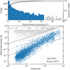 |
Fig. 4 Comparison of the uncertainty on the periods with the periods. |
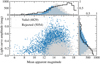 |
Fig. 5 Distribution of the validated and rejected samples against light curve amplitude and apparent magnitude. The black lines represent the fraction of rejected asteroids in the entire sample. |
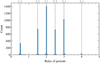 |
Fig. 6 Ratio of periods between ambiguous solutions. The vertical dashed lines indicate the ratio of integers. |
5 Validation
We assessed the quality of the periods determined here with three comparisons: the original TSSYS-DR1 results of Pál et al. (2020), the rotation periods on an independent extraction of TESS photometry by McNeill et al. (2023), and other values from the literature (providing periods from altogether different data sets). As visible in Fig. 7, there is a significant spread among periods when comparing the present determinations with those from Pál et al. (2020). It, however, mainly concerns rejected periods. Among the validated solutions (4829, i.e., 48.8% of the sample), the comparison is much better and 78.5% of the solutions agree within 1%. Another 3.6% correspond to period aliases (half or double period). The comparison with McNeill et al. (2023) presents a larger spread, even in the validated solutions (3601, i.e., 40.0% of the common sample). Overall, 63.1% of the solutions agree within one percent and an additional 2.9% correspond to period aliases. While based on similar original TESS data, the two studies extracted the photometry and determined the period using different methods, explaining the differences observed here. In their study, McNeill et al. (2023) actually reported numerous cases of disagreement with Pál et al. (2020), while about 80% of solutions agreed. For instance, while mainly periods reported by Pál et al. (2020) correspond to either half or twice the period reported here (Fig. 7), those reported by McNeill et al. (2023) almost never correspond to half the period reported here.
We then made a comparison with periods reported by other authors on different data sets (excluding TESS). We thus compiled the rotation period for each asteroid in our sample, using the ssoCard of SsODNet1 through its rocks2 interface (Berthier et al. 2023). We focus on period determinations with a quality flag of 3, that is, those that are deemed definitive, following the criterion by LCDB (Warner et al. 2009). As visible on Fig. 7, there is globally a better agreement with 1483 period determinations (for 670 unique asteroids). We find 91.0% agreeing within one percent, with additional 0.9% corresponding to aliases. This highlights the robustness of the method used here to select the period among the different possible solution (Sect. 3).
There are three main advantages of the technique presented in the present study. First, we considered several number of Fourier series, while also taking into account the number of local maxima (there should be at least two local maxima, otherwise we would be doubling the period). We assume that the light curve is a result of the shape features. In Fig. 3 one can see the result for asteroid (511) Davida. The period is clearly determined and in agreement with many previous studies from ground-based light curve observations (e.g., De Angelis 1995; Torppa et al. 2003; Cellino et al. 2019; Vernazza et al. 2021); however, at least the third order of a Fourier series is required. The result for the second order is twice smaller and coincides with Pál et al. (2020). Our explanation for this is that the light curve is quite π- periodic, on the one hand, and it does not resemble a cosine, on the other hand. Therefore the second-order Fourier series with twice smaller period can fit the contour of the light curve much better, but once we take third-order Fourier series, the difference between the two peaks of the light curve becomes important.
Second, we checked the number of local extrema. We illustrate this second advantage with asteroid (699) Heia in Fig. 3. The lower part of the figure shows that there is two possible solutions with radically different frequencies. However, the second frequency of 14.13 cycles/day provides only one local maxima and hence its period should be multiplied by 2, yielding the same fit to the data.
Finally, we did not just provide the chosen solution, but all the possible solutions. Sometimes there can be two or three possible solutions (periods for which σ is not significantly higher). These periods are also possible and we report their values. For some asteroids, the data are not accurate enough to obtain reliable results and the range of possible rotational periods ends up including the entire possible interval: from 2 to 360 h. This interval helps us understand the quality and reliability of the result. In the case of asteroid 2014 AX12 (Fig. 3), the uncertainty in the photometry is so high that almost any period can be fitted. The uncertainty interval for this asteroid is [2h, 237 h]. This basically means that the result should not be considered, even though there is a formal solution associated with the minimal value of σ.
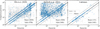 |
Fig. 7 Comparison of rotation periods found here with those derived by Pál et al. (2020) (9912, lleft) by McNeill et al. (2023) (6635, center) and gathered from the literature (1483 periods for 670 asteroids, right). The black line represents full agreement and the dashed gray lines the aliases for double and half periods. |
6 Discussion
We present in Fig. 8 how periods derived here are distributed against the diameter measurements. We also present data compiled from the literature (retrieved from SsODNet, Berthier et al. 2023). The limits imposed by TESS observations are clearly visible. First, the cadence of exposures (30 min) and length of observations (27 days) limit the range of periods that can be determined (Sect. 3), between 1 h and 27 days. Second, there is a clear drop in the amount of solutions below a diameter of 2–3 km. This diameter roughly corresponds to an apparent magnitude of 18 in the asteroid belt, which is indeed the peak in the magnitude distribution in TSSYS-DR1 data set (Pál et al. 2020). This distribution, combined with the trend for faintest asteroids to have the highest rejection rate (Fig. 5), explains the drop of solutions below 2–3 km in diameter.
The lower limit of 1 h is not reached by any of our solutions. As also visible in the data from the literature, there is a clear boundary at 2.2h which is refereed to as the “spin barrier” and corresponds to the critical rotation period at which self gravity and centrifugal acceleration are balanced (Pravec & Harris 2000). The situation is different for the upper limit, with longer rotation periods reported in the literature from long-term campaigns of observation or archival data (e.g., Waszczak et al. 2015; Erasmus et al. 2021; Marciniak et al. 2021). We note the presence of a valley around 50–100 h separating the bulk of fast rotators from the slower ones, with an apparent dependence on diameter. This low-density region was already visible in the rotation periods determined from K2 by Kalup et al. (2021) and from Gaia by Ďurech & Hanuš (2023).
We present in Fig. 9 the distribution of the amplitude of the light curves as a function of the asteroid diameter. We also present the asteroids reported in the LCDB (Warner et al. 2009) for comparison. Most asteroids have a diameter between 3 and 20 km. There is a clear trend of higher light-curve amplitudes toward smaller diameters, revealed by the running average. Such a trend was already visible in the results of the Palomar Transient Factory on asteroids (Waszczak et al. 2015). The amplitude of the light curve is directly related to the change of the projected area of the shape on the plane of the sky. Smaller amplitudes are thus indicative of rounder shapes. The trend here is a clear signature of asteroids being less spherical at smaller diameters. Such a trend has been reported from the results of 3D shape modeling of the 42 of the largest (diameter above 100 km) main belt asteroids, with an increase of asphericity toward smaller diameters (Vernazza et al. 2021). The regular increase in amplitude below the 100 km reveals that the trend continues down to diameters as small as 2 km (size at which the present data set is limited).
We compare the light-curve amplitude to the rotation period in Fig. 10, focusing on the shortest rotation periods. The period distribution is not random, with a limit at the shortest periods dependent on the amplitude of the light curve. As a guideline, we present the theoretically largest possible amplitude for bodies held together by self-gravity only (taken from, Waszczak et al. 2015) for three reference densities: 1000, 2000, and 3000 kg m−3. There is a clear difference between asteroids in a broad “S” complex (including the S, Q, A, V, E classes) and those in a broad “C” complex (C, Ch, B, D, P, Z classes, see Mahlke et al. 2022, for a rationale on this grouping), as expected from the higher density of the first group. The fraction of S-like asteroids is higher below the spin limit of 1000 kg m−3, revealing the lower density of C-like asteroids (below or slightly above 1000 kg m−3) compared to S-like asteroids, closer to 2000 kg m−3.
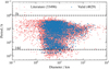 |
Fig. 8 Distribution of the rotation period as function of the asteroid diameter, compared with the literature. The two horizontal dashed lines represent the minimum and maximum periods that can be determined here (Sect. 3). |
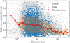 |
Fig. 9 Distribution of the light-curve amplitude as a function of asteroid diameter. The asteroids in LCDB (Warner et al. 2009) are plotted for reference, as well as a running mean (red line) and standard deviation (shaded area). |
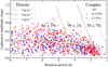 |
Fig. 10 Distribution of amplitude against rotation period. The gray lines represent the fastest spin for bodies held together solely by self-gravity from Waszczak et al. (2015). The fraction of S-types among all asteroids is indicated between those curves. |
7 Conclusion
We present a new approach of determining the rotational period of asteroids from optical light curves. The key aspects of the approach are:
Fit of Fourier series to the data by the least-squares method.
Selection of the model with the lowest weighted root-mean square residuals.
Selection of the lowest possible order of Fourier series, following the principle of “the less the better”.
Check with the F-test if higher orders Fourier series are necessary.
Test the number of local maxima of the function. Multiply the period by two if only one local maxima is present (we assume that the shape mostly produces the light curve).
Report the determined rotation period with its uncertainties. This includes the confidence interval of the period and the possible alternative rotational periods (ambiguous solutions with similar residuals, generally alises of the solution). If there are too many alternative periods, an interval encompassing all these periods is reported.
This approach was used to compute the rotational periods of asteroids observed by Transiting Exoplanet Survey Satellite (TESS) reported by Pál et al. (2020). This dataset has observations of 9912 asteroids. We determined the period of 4521 asteroids with an accuracy better than 10%.
Comparison of our results with Pál et al. (2020) shows 78.5% of a full agreement. For some of the asteroids, we identified the advantage of our technique, in particular, when fitting higher order of Fourier series and checking for the number of local maxima. The method we propose here is robust and can be applied to any dataset of dense light curves of asteroids. Thus, we plan to use it on available asteroid datasets in a future work.
Data availability
The catalog is available at the CDS via anonymous ftp to cdsarc.cds.unistra.fr (130.79.128.5) or via https://cdsarc.cds.unistra.fr/viz-bin/cat/J/A+A/693/A66
Acknowledgements
B.C. acknowledges support by the French ANR, project T- ERC SolidRock (ANR-20-ERC8-0003). This paper includes data collected by the TESS mission. Funding for the TESS mission is provided by the NASA Explorer Program. We did an extensive use of the VO tools TOPCAT (Taylor 2005) and SsODNet (Berthier et al. 2023). Thanks to all the developers and maintainers.
References
- Berthier, J., Carry, B., Vachier, F., Eggl, S., & Santerne, A. 2016, MNRAS, 458, 3394 [NASA ADS] [CrossRef] [Google Scholar]
- Berthier, J., Carry, B., Mahlke, M., & Normand, J. 2023, A&A, 671, A151 [NASA ADS] [CrossRef] [EDP Sciences] [Google Scholar]
- Bottke, W. F., Vokrouhlický, D., Broz, M., Nesvorný, D., & Morbidelli, A. 2001, Science, 294, 1693 [NASA ADS] [CrossRef] [Google Scholar]
- Bowell, E., Hapke, B., Domingue, D., et al. 1989, in Asteroids II, eds. R. P. Binzel, T. Gehrels, & M. S. Matthews (Tucson: University of Arizona Press), 524 [Google Scholar]
- Cellino, A., Hestroffer, D., Lu, X. P., Muinonen, K., & Tanga, P. 2019, A&A, 631, A67 [NASA ADS] [CrossRef] [EDP Sciences] [Google Scholar]
- Clement, M. S., Morbidelli, A., Raymond, S. N., & Kaib, N. A. 2020, MNRAS, 492, L56 [NASA ADS] [CrossRef] [Google Scholar]
- De Angelis, G. 1995, Planet. Space Sci., 43, 649 [CrossRef] [Google Scholar]
- DeMeo, F. E., & Carry, B. 2014, Nature, 505, 629 [NASA ADS] [CrossRef] [Google Scholar]
- Ďurech, J., Carry, B., Delbo, M., Kaasalainen, M., & Viikinkoski, M. 2015, Asteroid Models from Multiple Data Sources (Tucson: University of Arizona Press), 183 [Google Scholar]
- Ďurech, J., & Hanuš, J. 2023, A&A, 675, A24 [NASA ADS] [CrossRef] [EDP Sciences] [Google Scholar]
- Erasmus, N., Kramer, D., McNeill, A., et al. 2021, MNRAS, 506, 3872 [NASA ADS] [CrossRef] [Google Scholar]
- Eyer, L., & Bartholdi, P. 1999, A&AS, 135, 1 [NASA ADS] [CrossRef] [EDP Sciences] [Google Scholar]
- Grice, J., Snodgrass, C., Green, S., Parley, N., & Carry, B. 2017, Asteroids, Comets, and Meteors: ACM 2017 [Google Scholar]
- Gubanov, V. C. 1997, Obobshchennyj metod naimen’shih kvadratov. Teoriya i primeneniya v astrometrii. (in Russian. Generalized method of least squares. Theory and application in astrometry.) (Nauka) [Google Scholar]
- Hirayama, K. 1918, AJ, 31, 185 [Google Scholar]
- Kaasalainen, M. 2004, A&A, 422, L39 [NASA ADS] [CrossRef] [EDP Sciences] [Google Scholar]
- Kaasalainen, M., Torppa, J., & Muinonen, K. 2001, Icarus, 153, 37 [NASA ADS] [CrossRef] [Google Scholar]
- Kalup, C. E., Molnár, L., Kiss, C., et al. 2021, ApJS, 254, 7 [NASA ADS] [CrossRef] [Google Scholar]
- Linnik, Y. V. 1961, Method of Least Squares and Principles of Theory of Observations (translated from Russian by R. C. Elandt), ed. N. L. Johnson (Oxford, UK: Pergamon Press) [Google Scholar]
- Mahlke, M., Carry, B., & Denneau, L. 2021, Icarus, 354, 114094 [Google Scholar]
- Mahlke, M., Carry, B., & Mattei, P. A. 2022, A&A, 665, A26 [NASA ADS] [CrossRef] [EDP Sciences] [Google Scholar]
- Marciniak, A., Durech, J., Alí-Lagoa, V., et al. 2021, A&A, 654, A87 [NASA ADS] [CrossRef] [EDP Sciences] [Google Scholar]
- Masiero, J. R., Mainzer, A. K., Grav, T., et al. 2011, ApJ, 741, 68 [Google Scholar]
- McNeill, A., Gowanlock, M., Mommert, M., et al. 2023, AJ, 166, 152 [NASA ADS] [CrossRef] [Google Scholar]
- Milani, A., Cellino, A., Kneževic, Z., et al. 2014, Icarus, 239, 46 [NASA ADS] [CrossRef] [Google Scholar]
- Morbidelli, A., Walsh, K. J., O’Brien, D. P., Minton, D. A., & Bottke, W. F. 2015, The Dynamical Evolution of the Asteroid Belt, eds. P. Michel, F. DeMeo, & W. F. Bottke (Tucson: University of Arizona Press), 493 [Google Scholar]
- Muinonen, K., Belskaya, I. N., Cellino, A., et al. 2010, Icarus, 209, 542 [Google Scholar]
- Pál, A., Szakáts, R., Kiss, C., et al. 2020, ApJS, 247, 26 [CrossRef] [Google Scholar]
- Pravec, P., & Harris, A. W. 2000, Icarus, 148, 12 [NASA ADS] [CrossRef] [Google Scholar]
- Scheirich, P., & Pravec, P. 2009, Icarus, 200, 531 [NASA ADS] [CrossRef] [Google Scholar]
- Taylor, M. B. 2005, ASP Conf. Ser., 347, 29 [Google Scholar]
- Tedesco, E. F., Noah, P. V., Noah, M. C., & Price, S. D. 2002, AJ, 123, 1056 [NASA ADS] [CrossRef] [Google Scholar]
- Torppa, J., Kaasalainen, M., Michalowski, T., et al. 2003, Icarus, 164, 346 [NASA ADS] [CrossRef] [Google Scholar]
- Usui, F., Kuroda, D., Müller, T. G., et al. 2011, PASJ, 63, 1117 [Google Scholar]
- Vernazza, P., Ferrais, M., Jorda, L., et al. 2021, A&A, 654, A56 [NASA ADS] [CrossRef] [EDP Sciences] [Google Scholar]
- Vokrouhlický, D., Bottke, W. F., Chesley, S. R., Scheeres, D. J., & Statler, T. S. 2015, Asteroids IV, The Yarkovsky and YORP Effects, eds. P. Michel, F. DeMeo, & W. F. Bottke (Tucson: University of Arizona Press), 509 [Google Scholar]
- Warner, B. D., Harris, A. W., & Pravec, P. 2009, Icarus, 202, 134 [NASA ADS] [CrossRef] [Google Scholar]
- Waszczak, A., Chang, C.-K., Ofek, E. O., et al. 2015, AJ, 150, 75 [NASA ADS] [CrossRef] [Google Scholar]
- Zappala, V., Cellino, A., Farinella, P., & Kneževic, Z. 1990, AJ, 100, 2030 [CrossRef] [Google Scholar]
All Figures
|
Fig. 1 Top: distribution of the maximal, minimal, and range of phase angles. Bottom: range of phase as a function of the minimum phase angle. |
| In the text | |
|
Fig. 2 Example of light curve fit for asteroid (3) Juno. Top: TSSYS-DR1 data as function of time. Observations are plotted as dots, color-coded by epoch. Crosses represent data rejected by the fitting procedure (see text). The line represents the best fit. Middle: same as above, folded over a rotation period ( |
| In the text | |
|
Fig. 3 Illustrations of the advantages of the method (symbols are the same as Fig. 2). Left: clear period determination, but it would be (erroneously) twice smaller if only the second order of the Fourier series was used. Center: two solutions with acceptable sigma values but corresponding to the same period – if the number of local maxima is taken into account. Right: all solutions below the significance level, thus, the uncertainty interval is 2–237 h, i.e., the period is not determined. |
| In the text | |
|
Fig. 4 Comparison of the uncertainty on the periods with the periods. |
| In the text | |
|
Fig. 5 Distribution of the validated and rejected samples against light curve amplitude and apparent magnitude. The black lines represent the fraction of rejected asteroids in the entire sample. |
| In the text | |
|
Fig. 6 Ratio of periods between ambiguous solutions. The vertical dashed lines indicate the ratio of integers. |
| In the text | |
|
Fig. 7 Comparison of rotation periods found here with those derived by Pál et al. (2020) (9912, lleft) by McNeill et al. (2023) (6635, center) and gathered from the literature (1483 periods for 670 asteroids, right). The black line represents full agreement and the dashed gray lines the aliases for double and half periods. |
| In the text | |
|
Fig. 8 Distribution of the rotation period as function of the asteroid diameter, compared with the literature. The two horizontal dashed lines represent the minimum and maximum periods that can be determined here (Sect. 3). |
| In the text | |
|
Fig. 9 Distribution of the light-curve amplitude as a function of asteroid diameter. The asteroids in LCDB (Warner et al. 2009) are plotted for reference, as well as a running mean (red line) and standard deviation (shaded area). |
| In the text | |
|
Fig. 10 Distribution of amplitude against rotation period. The gray lines represent the fastest spin for bodies held together solely by self-gravity from Waszczak et al. (2015). The fraction of S-types among all asteroids is indicated between those curves. |
| In the text | |
Current usage metrics show cumulative count of Article Views (full-text article views including HTML views, PDF and ePub downloads, according to the available data) and Abstracts Views on Vision4Press platform.
Data correspond to usage on the plateform after 2015. The current usage metrics is available 48-96 hours after online publication and is updated daily on week days.
Initial download of the metrics may take a while.