| Issue |
A&A
Volume 679, November 2023
|
|
|---|---|---|
| Article Number | A60 | |
| Number of page(s) | 43 | |
| Section | Catalogs and data | |
| DOI | https://doi.org/10.1051/0004-6361/202346191 | |
| Published online | 07 November 2023 | |
Scaling slowly rotating asteroids with stellar occultations★
1
Astronomical Observatory Institute, Faculty of Physics, Adam Mickiewicz University,
Sloneczna 36,
60-286
Poznań, Poland
e-mail: am@amu.edu.pl
2
Astronomical Institute, Faculty of Mathematics and Physics, Charles University,
V Holešovičkách 2,
180 00
Prague 8, Czech Republic
3
Mt. Suhora Observatory, Pedagogical University,
Podchorążych 2,
30-084
Cracow, Poland
4
Konkoly Observatory, Research Centre for Astronomy and Earth Sciences, Eötvös Loránd Research Network (ELKH),
1121
Budapest,
Konkoly Thege Miklós út 15-17, Hungary
5
CSFK, MTA Centre of Excellence, Budapest,
Konkoly Thege Miklós út 15-17,
1121,
Hungary
6
MTA CSFK Lendület Near-Field Cosmology Research Group,
Hungary
7
ELTE Eötvös Loránd University, Institute of Physics,
1117, Pázmány Péter sétány 1/A,
1117
Budapest, Hungary
8
Astronomy Department, Eötvös Loránd University,
Pázmány P. s. 1/A,
1171
Budapest, Hungary
9
Observatorio Nacional,
R. Gen. José Cristino 77, Säo Cristövão,
20921-400,
Rio de Janeiro, RJ, Brazil
10
EURASTER,
8 rue du Tonnelier,
46100
Faycelles, France
11
International Occultation Timing Association/European Section,
Am Brombeerhag 13,
30459
Hannover, Germany
12
International Occultation Timing Association (IOTA),
PO Box 7152,
WA
98042,
USA
13
Institute of Theoretical Physics and Astronomy, Vilnius University,
Saulėtekio al. 3,
10257
Vilnius, Lithuania
14
Japanese Occultation Information Network,
Japan
15
Geneva Observatory,
1290
Sauverny, Switzerland
16
Les Engarouines Observatory,
84570
Mallemort-du-Comtat, France
17
Association T60, Observatoire Midi-Pyrénées,
14 avenue Édouard Belin,
31400
Toulouse, France
18
Collonges Observatory,
90 allée des Résidences,
74160
Collonges, France
19
Institute of Astronomy, Faculty of Physics, Astronomy and Informatics, Nicolaus Copernicus University in Toruń,
ul. Grudziądzka 5,
87-100
Toruń, Poland
20
Departamento de Sistema Solar, Instituto de Astrofísica de Andalucía (CSIC),
Glorieta de la Astronomía s/n,
18008
Granada, Spain
21
Observatoire du Bois de Bardon,
16110
Taponnat, France
22
Arecibo Observatory, University of Central Florida,
HC-3 Box 53995,
Arecibo, PR
00612, USA
23
Instituto de Astrofisica de Canarias,
C/ Via Lactea, s/n,
38205
La Laguna, Tenerife, Spain
24
Gran Telescopio Canarias (GRANTECAN),
Cuesta de San José s/n,
38712,
Brena Baja, La Palma, Spain
25
Open University, School of Physical Sciences, The Open University,
MK7 6AA, UK
26
Trans-Tasman Occultation Alliance (TTOA),
Wellington,
PO Box 3181, New Zealand
27
Hunters Hill Observatory,
7 Mawalan Street,
Ngunnawal,
ACT 2913, Australia
28
Space sciences, Technologies and Astrophysics Research Institute, Université de Liège,
Allée du Août
4000
Liège, Belgium
29
British Astronomical Association, Burlington House, Piccadilly, Mayfair,
London
W1J 0DU, UK
30
Institute of Physics, Jan Kochanowski University,
ul. Uniwersytecka 7,
25-406
Kielce, Poland
31
Chungbuk National University,
1, Chungdae-ro, Seowon-gu, Cheongju-si,
Chungcheongbuk-do, Republic of Korea
32
Korea Astronomy and Space Science Institute,
776 Daedeok-daero, Yuseong-gu,
Daejeon
34055, Korea
33
Laboratory of Space Researches, Uzhhorod National University,
Daleka st. 2a,
88000,
Uzhhorod, Ukraine
34
Departamento de Astrofisica, Universidad de La Laguna - ULL,
Tenerife, Spain
35
NASA Johnson Space Center Astronomical Society,
Houston, TX
77058, USA
36
Blue Mountains Observatory,
94 Rawson Parade,
Leura
NSW 2780, Australia
37
Organ Mesa Observatory,
4438 Organ Mesa Loop,
Las Cruces, NM
88011, USA
38
Command Module Observatory,
121 W. Alameda Dr.,
Tempe, AZ
85282, USA
39
Silesian University of Technology, Department of Electronics, Electrical Engineering and Microelectronics,
Akademicka 16,
44-100
Gliwice, Poland
40
Lowell Observatory,
1400 West Mars Hill Road,
Flagstaff, AZ
86001, USA
41
Department of Astronomy, University of Virginia,
Charlottesville, VA
22904, USA
42
Department of Physics, Adiyaman University,
02040
Adiyaman, Turkey
43
Observatory,
Vsetínská 78,
757 01
Valašské Meziříčí, Czech Republic
44
Kepler Institute of Astronomy, University of Zielona Góra,
Lubuska 2,
65-265
Zielona Góra, Poland
Received:
20
February
2023
Accepted:
28
August
2023
Context. As evidenced by recent survey results, the majority of asteroids are slow rotators (spin periods longer than 12 h), but lack spin and shape models because of selection bias. This bias is skewing our overall understanding of the spins, shapes, and sizes of asteroids, as well as of their other properties. Also, diameter determinations for large (>60 km) and medium-sized asteroids (between 30 and 60 km) often vary by over 30% for multiple reasons.
Aims. Our long-term project is focused on a few tens of slow rotators with periods of up to 60 h. We aim to obtain their full light curves and reconstruct their spins and shapes. We also precisely scale the models, typically with an accuracy of a few percent.
Methods. We used wide sets of dense light curves for spin and shape reconstructions via light-curve inversion. Precisely scaling them with thermal data was not possible here because of poor infrared datasets: large bodies tend to saturate in WISE mission detectors. Therefore, we recently also launched a special campaign among stellar occultation observers, both in order to scale these models and to verify the shape solutions, often allowing us to break the mirror pole ambiguity.
Results. The presented scheme resulted in shape models for 16 slow rotators, most of them for the first time. Fitting them to chords from stellar occultation timings resolved previous inconsistencies in size determinations. For around half of the targets, this fitting also allowed us to identify a clearly preferred pole solution from the pair of two mirror pole solutions, thus removing the ambiguity inherent to light-curve inversion. We also address the influence of the uncertainty of the shape models on the derived diameters.
Conclusions. Overall, our project has already provided reliable models for around 50 slow rotators. Such well-determined and scaled asteroid shapes will, for example, constitute a solid basis for precise density determinations when coupled with mass information. Spin and shape models in general continue to fill the gaps caused by various biases.
Key words: minor planets, asteroids: general / techniques: photometric
Lighcurves are available at the CDS via anonymous ftp to cdsarc.cds.unistra.fr (130.79.128.5) or via https://cdsarc.cds.unistra.fr/viz-bin/cat/J/A+A/679/A60
© The Authors 2023
 Open Access article, published by EDP Sciences, under the terms of the Creative Commons Attribution License (https://creativecommons.org/licenses/by/4.0), which permits unrestricted use, distribution, and reproduction in any medium, provided the original work is properly cited.
This article is published in open access under the Subscribe to Open model. Subscribe to A&A to support open access publication.
1 Introduction
One of the ultimate aims of asteroid research is to obtain density determinations that would enable studies of their internal structure (micro- and macroporosity), and mineralogical composition in order to link meteorites with their parent bodies. Asteroids larger than 100 km in diameter are considered primitive and largely unchanged since their formation (Morbidelli et al. 2009), while smaller ones are seen as remnants of collisional disruptions and reaccumulations, with substantial macroporosity (Carry 2012).
Sizes of asteroids, a necessary prerequisite to deriving conclusions as to internal structure and density where mass is available, are not easy to determine. Accurate size determinations are of vital importance, as their relative error is tripled in density determinations, while to clearly distinguish between the different mineralogies of asteroid interiors, the density needs to be known with 20% precision (Carry 2012). In the majority of cases, asteroid sizes are calculated from a known value of absolute magnitude, and an assumed geometric albedo (Harris & Harris 1997), which leads to large uncertainties in the derived diameter, namely at the level of 20%–30% for main-belt asteroids, and reaching over 50% in some cases (Tanga et al. 2013)1. The solution is to use infrared measurements: in the visible light, a small target with a highly reflective surface is equally as bright as a large target with a dark surface. However, in the infrared, the two objects appear substantially different. A visually dark object, due to its smaller albedo, absorbs most of the solar radiation, and is heated to higher temperatures than its visually brighter counterpart (Harris & Lagerros 2002). Therefore, thermal data combined with absolute brightness in the visible light enable us to put tight constraints on the object size, typically reducing the uncertainty to 5–10% (Delbo’ et al. 2015), but only if spin and shape model is available. Without a model, the accuracy of this method is greatly reduced. Also, this method is limited to objects with rich thermal datasets from multiple space observatories. For example, large objects of around 100 km in diameter tend to be saturated in W3 and/or W4 bands (11.1 and 22.64 μm respectively) of the WISE mission (Wright et al. 2010), and so data from WISE cannot be used in their thermophysical modelling (Delbo’ et al. 2015). The diameters of these targets must therefore be determined with other methods.
A somewhat complementary method that enables large asteroid surfaces to be imaged and their shapes and sizes to be determined is high-resolution imaging with the state-of-the-art adaptive optics systems used with modern deconvolution techniques. A recent large programme at the VLT using the SPHERE/ZIMPOL instrument provided detailed shapes and accurate sizes for around 40 main-belt asteroids representing all of the main taxonomic classes (see e.g. Vernazza et al. 2021). This technique, although spectacular, is nevertheless limited to the relatively nearby and large asteroids.
Another powerful technique for measuring sizes of asteroids is the stellar occultation timing analysis (Herald et al. 2020), which is almost completely independent of their size or distance. Asteroids in their on-sky paths sometimes cross background stars, casting a shadow on the Earth surface. Observations of these rare events from a few separate sites within the predicted shadow path – thanks to precise timings – enable almost direct asteroid size measurements in kilometers. The target silhouette can also be outlined by the occultation, which can be used to verify the shape models (Ďurech et al. 2011). Such events sometimes lead to discoveries of asteroid satellites or rings (Gault et al. 2022; Ortiz et al. 2017), enabling mass determinations. An important advantage of this technique is the possibility to break the symmetry between two mirror pole solutions, which is inherent to photometric light-curve inversions of asteroids orbiting close to the ecliptic plane (Kaasalainen & Lamberg 2006).
A desirable situation would be to have at least three occultation chords for each event (Ďurech et al. 2011). A dense network of ground-based observatories is therefore required, such as the network built within the Lucky Star project2, the RECON network3 (Buie & Keller 2016), or the wide and well-organised regional networks of the International Occultation Timing Association4. With Gaia catalogues available (Gaia Collaboration 2021), the accuracy of occultation predictions has substantially improved (Tanga et al. 2022), and is expected to improve even more with the release of the full Gaia catalogue. Now there is a unique opportunity for successful observations, since both stellar positions and asteroid orbits are determined with unprecedented accuracy, resulting in most reliable occultation predictions to date. There is a time-window in which to take this opportunity, because over the following decades both quantities will start to deteriorate because of uncertainties in stellar proper motions and perturbations of asteroid orbits.
The vast majority of asteroid shape models published today are scale-free, approximate shape representations, because the focus is mainly on determining their spin parameters (see e.g. Hanuš et al. 2018; Ďurech et al. 2020). These shape models, given their angular appearance with sharp edges and large planar areas, tend to be problematic when used in further applications such as thermophysical modelling or fitting their silhouettes to stellar occultations (Hanuš et al. 2016), with the main outcome of both being diameter determinations.
In parallel, the targets on which most of these studies have focused do not necessarily represent all of the various populations of main-belt asteroids (Marciniak et al. 2015). Most of the spin and shape asteroid models available today are for relatively fast-rotating targets, while the TESS mission, for example, revealed that slow rotators (bodies rotating with periods of longer than 12 h) strongly dominate in all asteroid populations at various sizes (e.g. around 5700 objects out of 9900 in the TESS DR1 sample5, Pál et al. 2020).
Motivated by the trends described above, our survey (see e.g. Marciniak et al. 2018) is designed to reconstruct precise spin and three-dimensional shape models for the most challenging, slowly rotating asteroids, and to determine their sizes with the best available methods (thermophysical modelling, and/or stellar occultation fitting). Thanks to this survey, we now have the most accurate shape models and size values to date for over 30 such asteroids (Marciniak et al. 2021). In this work, we present a further 16 slow rotators, most of which previously lacked shape models or even good-quality light curves. Unlike our previous targets (published in Marciniak et al. 2018, Marciniak et al. 2019, 2021), these 16 asteroids could not be reliably scaled using thermal data because of the poor quality of the infrared datasets existing for them. Here, we therefore focus on scaling them using stellar occultations.
Section 2 describes our two observing campaigns, which target these bodies: one to obtain their light curves in multiple apparitions, and another to observe them in stellar occultations. Sections 3 and 4 present the methods we used for shape reconstruction and to fit the models to stellar occultation chords. Section 5 presents asteroid spin and shape models, verified and scaled using occultation fitting, which in many cases enabled us to identify a preferred pole solution. A final section summarises our findings and presents future plans, with possible applications of our results.
2 Observing campaigns
2.1 Photometric campaign for dense light curves
Our wide photometric campaign, which is described in detail in Marciniak et al. (2015), is motivated by the lack of a good-quality representation of the main-belt asteroid population as a whole by spin and shape models. As expected, models have mainly been constructed for targets for which this process is relatively straightforward, while others have been left behind. Therefore, we focused on asteroids with long periods and low amplitudes in order to counterbalance this unequal distribution. Later, slow rotators were shown to be important targets for thermal studies, as it has been speculated that they might allow us to study deeper surface regolith layers (see Harris & Drube 2016, 2020; Marciniak et al. 2021, for discussions). Furthermore, as evident from the results from Kepler (Molnár et al. 2018; Kalup et al. 2021) and confirmed by TESS missions (Pál et al. 2020), the main focus in asteroid physical studies should be on slow rotators.
The light-curve campaign for slow rotators relies on a wide, relatively uniformly distributed, and efficiently coordinated network of small telescopes of up to 1m in diameter (Table B.1 in the Appendix presents the observing runs, sites, and participating observers). This allows full coverage of the light curves of targets with rotation periods reaching 60 h within a reasonable time-frame. Data collection took a long time, partly because of the long periods of our targets, but also because of the paucity of previous data, which meant it was necessary to observe each target in five or more apparitions in order to obtain a unique spin and shape model using the convex inversion method by Kaasalainen et al. (2001). Wherever possible, our light curves are supplemented with data from the Kepler and TESS missions, and from previous ground-based observations, resulting in dense light curves (see Table B.1 in the Appendix for references), mostly through the ALCDEF database6.
2.2 Stellar occultation campaign
In October 2020, we launched an auxiliary campaign for slow rotators. Although some of them have previously been observed in stellar occultations, the results were mostly single positive chord observations, which are unusable for precise scaling (Herald et al. 2019). Therefore, in cooperation with the European Section of the International Occultation Timing Association (IOTA/ES), we started an occultation campaign for ‘Neglected Asteroids’7. Later, this campaign gained its separate tag in the Occult Watcher Cloud8, a tool widely used for occultation planning and coordination. The aim is to register multi-chord stellar occultations for slow rotators from our target list. In contrast to the light-curve campaign, where hundreds of hours on-target are needed, occultation events require observations of only one or 2 min, as they last only a few seconds. This means that good coordination and timing are even more important than in the light-curve campaign. The occultation predictions were made using the JPL Horizons database for asteroid orbits9, and Gaia EDR310 for star positions. Although these events are rare, the campaign has already resulted in a dozen or so successful occultation observations, with the number of positive chords per event reaching nine (see e.g. the events from the years 2021 and 2022 in Figs. A.6 and A.14).
Archival occultation data were downloaded from the Planetary Data System (PDS) archive11 (Herald et al. 2019), and more recent ones were obtained from the archive of the Occult pro-gramme12, or directly from the regional IOTA coordinators, who perform data evaluation and vetting in order to achieve good-quality and consistent occultation results. Most of the occultation observers are amateur astronomers, which makes this campaign a good example of a successful professional-amateur, or ‘pro-am’, collaboration. Table B.2 provides the observer names and site locations for each occultation event used here.
3 Convex inversion with shape regularisation
The majority of asteroid models presented in this work were constructed using the common convex inversion method of Kaasalainen & Torppa (2001); Kaasalainen et al. (2001). When light-curve data are sufficiently abundant to uniquely determine the sidereal rotation period and the pole direction, the shape model reconstructed from the Gaussian image is usually such that its rotation axis z is very close to the principal axis of the inertia tensor with the largest moment of inertia. Shapes that fit the data but strongly violate this condition have to be rejected as physically unacceptable solutions of the inverse problem. However, in some cases the data are so abundant that it is clear that, although the solution is correct, the shape is not physically acceptable. By ‘squeezing’ the shape along the rotation axis, the inertia tensor can be changed in such a way that its greatest axis is close to the rotation axis. However, this can only be done after the best-fit model is found, and we must also check whether or not this shrinking along the rotation axis affects the light-curve fit significantly.
When working with the Gaussian image during the optimisation, the shape is not known and we cannot regularise it to obtain the maximum moment of inertia around the rotation axis. However, even without computing the inertia tensor precisely, the shapes that are not rotating along the shortest axis are elongated along the z axis. This elongation means that the cross-section viewed from the pole direction is smaller than that from the equatorial view (xy plane). Although the 3D shape is not available during optimisation, the areas of surface facets and their normals are known, and so their projections can be computed. The regularisation term R that we introduce is
 (1)
(1)
where  are unit normals to surface elements of areas σi, and
  ,
,  ,
,  are unit vectors along the coordinate axes; the summation is over all N surface elements. The more extended the shape along the z axis, the higher R, and so the penalty function that is added to the χ2 is R2 times some weight w. By increasing w, the shape model is forced to have projected areas along the x and y axes that are smaller than along the z axis, which makes it more oblate and ensures physically correct rotation. This way, we were able to produce physically realistic shapes for (439) Ohio and (566) Stereoskopia, for which the standard light-curve inversion without regularisation led to unphysical shapes. With regularisation, the fit to the data remained almost the same (RMS changed from 0.0073 to 0.0074 for the example shown in Fig. 1), meaning that the dimension along the rotation axis was not constrained by the data, and the regularisation helped to produce realistic shapes without affecting the fit. A ‘negative regularisation’ mentioned in the following section means using the regularisation term 1/R2, which produces more stretched shapes when needed.
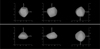 |
Fig. 1 Two versions of shape model 2 for (566) Stereoskopia: without shape regularisation (top) and with regularisation applied (bottom), using the same starting parameters otherwise. The three views show, from left to right: two equatorial views separated by 90°in phase, and the pole-on view. We note that the pole-on silhouettes generally agree between two versions of the shape model, as it is the equatorial cross-section that most effectively influences the light curves. |
4 Occultation fitting
As mentioned in Sect. 1, shape models derived from photometry do not carry information about the size; they are scale-free. We scaled them using the same approach as Ďurech et al. (2011) and recently Marciniak et al. (2021). The positions of the observers detecting an occultation were projected on the fundamental plane, which is the plane crossing the geocenter and is perpendicular to the direction from the asteroid to the star. We then computed the orientation of the shape model for the mean time of occultation and projected it also to the fundamental plane. Because the time span of occultation timings is usually much shorter than the rotation period of the asteroid, the rotation is neglected, and the silhouette is assumed to be constant. The size of the asteroid and the relative position of its projection on the fundamental plane with respect to chords are three parameters optimised to converge to the best agreement between the projection of the asteroid shape and occultation chords. The goodness of the fit is described by a standard χ2 measure with timing uncertainties taken into account.
The uncertainty of the derived size is affected by many factors: the number of occultation events, the number of chords in individual occultations and their distribution across the silhouette, the timing errors of individual chords, and the uncertainty on the projection of the asteroid (and therefore the uncertainty on its shape and spin state). When there are several occultations by one asteroid with many chords covering the whole projected disc, the RMS residual in kilometers is one estimation of the size uncertainty (see the last column in Table 1).
However, the uncertainty on the sizes of the asteroids determined in this way does not take into account the uncertainty on the models themselves. The main problem is that relative light curves supporting the models are largely insensitive to a vertical dimension of the shape model, as the ratio between the biggest and smallest projected area in a given aspect remains similar regardless of this dimension. To tackle this problem, we used the ability of inertia regularisation to influence the vertical stretch of the derived models. We created ten versions of each model, with both positive and negative regularisations, creating flatter and rounder shapes that would still fit the light curves at a similar level to the nominal solution, and at the same time remaining physical (rotating around the shortest axis) and realistic (e.g. not being extremely thin). Models fitting the light curves within 10% RMS of the best-fit solution are accepted following Kaasalainen et al. (2001). With tens of light curves and thousands of photometric points, the 10% increase in RMS is really an extreme limit and is the upper boundary for ‘acceptable’ models, as shown by the example in Fig. 2. The upper model is the nominal one, without inertia regularisation, while the bottom one was created with a relatively high level of regularisation. The other model fitted the light curves within 7% of the best solution (RMS of 0.0117 vs. 0.0110 for the best fit) and is already unrealistically flattened. Another approach relates the χ2 limit to the number of data points (see e.g. Hanuš et al. 2021; Ďurech et al. 2022, Appendix A).
Those variations of each model have been fitted to occultations as well, resulting in a pool of plausible sizes. This also revealed the shape versions fitting the occultations with substantially higher RMS, or not fitting some chords at all. In some cases, this strengthened the case for a preference for one of two pole solutions, where all the versions of shape for one pole resulted in a similar value for the size and a consistently small RMS of the fit, while for the other pole the sizes varied substantially, and the RMS was high. Such cases are described in more detail in the following section.
The key point here was to check whether the range of sizes derived in this way would be higher or smaller than the nominal RMS of the occultation fit, which is mainly governed by the occultation timing uncertainties. When it was higher, it replaced the nominal RMS value as a measure of diameter uncertainty in Table 1. However, when the range of sizes was smaller than the RMS of the fit, this meant that the uncertainty here was dominated by the occultation timing errors or the convex approximation of the shape.
Spin parameters and sizes of asteroid models obtained in this work.
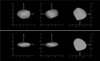 |
Fig. 2 Two versions of shape model 2 for (412) Elisabetha. The high-regularisation model (bottom) still fits the light curves on formally acceptable level, but is unrealistically flat. See Sect. 4 for discussion. |
5 Results
We used the rich datasets of dense light curves from our campaign (see Figs. C.1–C.77) for spin and shape modelling with the classical light-curve inversion method – or its slight variation with shape regularisation – in order to make non-physical models rotate in a physical manner around the axis of largest inertia (see Sect. 3). Table 1 summarises the spin parameters and diameters determined in this work. The fit of the shape models to occultation chords can be seen in Figs. 3–A.17. A good fit has manifold benefits: primarily it serves to scale the models in kilometers, but it also verifies the shape features, and often clearly points to the solution that must be close to the real one, making its mirror counterpart less probable. We should note that the asteroid sizes determined here are diameters of volume-equivalent spheres, while sizes determined from infrared measurements are for surface-equivalent spheres. In any case, the difference between the two diameters for the same shape model is at the level of 5% or less, which is smaller than the uncertainty on the models themselves, especially with NEATM spherical shape approximation. It is therefore justified to directly compare sizes determined with the two methods, without any scaling factors.
In parallel, in a few justified cases (275 Sapientia, 464 Megaira, 530 Turandot) where the occultation results suggest the presence of non-convex shape features, we additionally used the all-data asteroid modelling (ADAM, Viikinkoski et al. 2015) method for shape reconstruction. This technique uses both light curves and occultation timings as input data in a single optimisation process. The results are presented in Figs. 5, A.1, A.8, and A.12 and in Table 1. They can be compared with the respective shape models constructed with traditional convex inversion without occultations; and fitted to occultations later (Figs. 4, A.7, and A.11). The determined sizes and spin parameters are consistent between the two methods, while ADAM shapes show a slightly better fit to the occultations, as expected. The size uncertainties for ADAM shape models presented in Table 1 come from the scatter of solutions and are clearly underestimated.
For each model, Table 1 presents the spin axis ecliptic coordinates, with the sidereal period of rotation, together with the uncertainties on each parameter. The table also contains details of the light-curve datasets, and the volume-equivalent diameters with uncertainties based on the deviation of the shape model silhouettes from the occultation chord ends, or on the scatter of sizes for various versions of the same shape, whichever source dominated the error budget. The preferred pole solutions after occultation fitting are marked in boldface. In Figs. 3–A.17, lesser preferred solutions are marked with dashed magenta contours, and the solid blue contours mark the preferred solutions. In the case of only slightly preferred solutions, both contours are solid lines, but the preferred solution is still shown in blue. In some cases, the preference seems to be based on single chords, but it is the duration rather than the chord absolute position that is the deciding factor in such cases The duration of the occultation events is usually recorded correctly, while the gross timing error might shift the whole chord, but does not change its length. There are of course exceptions to this rule; see the discussion on (275) Sapientia in Sect. 5. In the cases with no preference for the spin solution, both coloured contours are again solid; see the text and figure captions for details.
Additionally, Table 2 contains the range of previously determined sizes, with the source references. Please note the diversity of the literature diameters, differing by 50% for some targets between different works. Below we describe all targets in more detail.
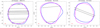 |
Fig. 3 (70) Panopaea model fit to occultation chords shown in the fundamental plane. North is up and west is right. Dashed lines mark visual observations, as opposed to video or photoelectric ones marked with solid lines. Grey segments correspond to timing uncertainties. Blue contour: Instantaneous silhouette of shape model 1 (see Table 1). Magenta: Same but for model 2. In this case, occultations show no preference for any of the models. |
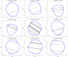 |
Fig. 4 (275) Sapientia model fit to occultation chords. Here, model 2 is preferred (blue solid contour). |
Previously published diameters for the asteroids studied here.
5.1 (70) Panopaea
Our result for the spin and shape of Panopaea (see Table 1) closely agrees with the one recently published by Hanuš et al. (2021). Three multi-chord occultations were available for Panopaea, one of them with a particularly rich set of 13 positive chords (see Fig. 3). However, many of these were visual observations, and the chords had unrealistically small error bars. All errors have been changed here to 0.05 s for photoelectric and video observations, and to 0.5 s for visual observations. Both shape solutions are consistent with the occultations, resulting in a size determination of 128 km with very small uncertainty of a few percent (Table 1). Previous literature diameter determinations for Panopaea varied widely from 105 km to 163 km (Table 2), and were mostly based on the NEATM model (Harris 1998), which approximates the body shape with a sphere.
5.2 (275) Sapientia
There were seven pre-existing occultation observations for this target (one with 16 chords), and our Neglected Asteroids campaign adds another two events. From the full set of nine events, four chords had to be removed because of their clear inconsistency with the remaining ones: there must have been large errors on either the duration or the absolute timing. The fitting to occultations clearly points at pole 2 as the preferred solution (Table 1), which is especially evident from the fit to occultations from years 2015, 2020, and 2021 (see Fig. 4). The size is determined with high accuracy (7%).
With such a rich set of occultations, and some of them suggesting non-convex shape features, the ADAM method was also applied. The resulting shape for pole 2 shows a slightly better fit to all occultations simultaneously (see Figs. 5 and A.1), but the fit is still not perfect. In particular, the four-chord event from the year 2018 cannot be fittted by any of the models, even though here we allow the occultations to influence the shape. The northernmost chord probably has an underestimated duration (this event is actually annotated ‘short low drop event in noisy recording’) or it points to some small shape feature below the resolution of the ADAM shape reconstruction procedure. The size of Sapi-entia found with the ADAM method (100 km) is consistent with that described above, and the scatter of possible sizes shrank to a mere 1%. Previous size determinations for Sapientia were somewhat less discrepant than for Panopaea, ranging from 89 to 124 km (Table 2).
5.3 (286) Iclea
Although the fit to the only available three-chord occultation for Iclea only slightly favours the pole 1 solution (see Fig. A.2), the sizes from the fitting for both solutions are clearly discrepant: the size for pole 2 solution is much smaller than the size for the pole 1 solution (69 vs. 86 km), and is also inconsistent with all the previous sizes determined using infrared data (81–125 km, see Table 2). Also, pole 1 spin parameters are confirmed by the results of Ďurech et al. (2020); this is the only solution for the pole of Iclea. Considering all of the above, we think that our solution for pole 2 (Table 1) can be safely rejected.
5.4 (326) Tamara
There exists an extremely wide range of literature diameters for Tamara (see Table 2): from 63 km to as much as 117 km, an almost two-fold difference. This might be due to the relatively unusual orbit of Tamara given that it is a main-belt asteroid, with an eccentricity of 0.19, and an inclination of 23°. As a consequence, thermal measurements of Tamara must have been taken at substantially varied heliocentric distances, complicating thermal analysis. Our result, being independent of thermal aspects, resolves these inconsistencies, pinpointing the diameter of this body to  km. The first pole solution is preferred based on the quality of the occultation fit (Fig. A.3), with the RMS being almost twice as low as in any version of model 2. Also, the spin solution found here is in good agreement with that from Hanuš et al. (2021).
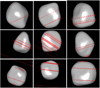 |
Fig. 5 (275) Sapientia, ADAM solution pole 1, shown with occultation chords used to construct the model. Occultation events are the same as in Fig. 4. |
5.5 (412) Elisabetha
The model 2 solution for Elisabetha is a much better fit to the occultations than any version of model 1 (compare the events from years 2011 and 2016 between the two poles in Fig. A.4), and therefore model 2 is our preferred solution (Table 1). Our size determination ( km) confirms previous determinations (76–112 km), which tended towards larger values (see Table 2, and MP3C database).
5.6 (426) Hippo
For Hippo we obtained two pole solutions from light-curve inversion; however, the second pole (see Table 1) was at the verge of rejection on the basis of the RMS fit to the light curves, which was almost 10% higher than for the first pole. See Sect. 4 for a discussion of this threshold. Our spin solutions roughly agree with those published by Hanuš et al. (2021) and Ďurech et al. (2019), in terms of pole latitude and period but disagree with the pole longitude for model 2 presented by these authors.
We decided to fit both shape solutions to the rich set of occultations; see Fig. A.5. Surprisingly, it is the shape connected to pole solution 2 (blue contour in Fig. A.5) that fits most of the occultations better than solution 2, especially the richest one from 27 December 2021. We therefore consider the pole 1 solution to be lesser probable (dashed magenta contour), even though it provided a formally better fit to light curves. The size determined here (122 ± 4 km) is close to the middle of the size range found in the literature (Table 2).
5.7 (439) Ohio
Our research into the asteroid Ohio is a success in multiple ways. First, we have been able to correct a previously accepted rotation period, identifying a period of around 37.46 h as the correct one (Marciniak et al. 2015), instead of 19.2 h which persisted for decades in the asteroid Light-Curve Database (Warner et al. 2009). Later, after gathering sufficient light-curve data over multiple apparitions, we managed to obtain its physically rotating model, which was possible thanks to regularisation added to light-curve inversion routines. There was only a single pole solution (Table 1) on the level of light-curve inversion, as the mirror pole solution gave a much poorer fit to light curves. This is facilitated by a relatively high orbital inclination of 19° for Ohio. Our spin solution is ~30° and ~50° away in spin axis latitude and longitude, respectively, from the pole 2 solution provided by Ďurech et al. (2018).
Later, in March 2022, we coordinated observers around two stellar occultation events (resulting in 6 and 9 positive chords, including one grazing event observed by the first author), where there were no previously recorded multi-chord events (i.e. containing more than three positive chords). In the end, our shape model was fitted to these occultations, presenting a very good-quality fit (see Fig. A.6). Thanks to the quality of both the model and the occultation timings, the shape was precisely scaled with small residual RMS. The only small discrepancies between the model and the chords from the last occultation probably reveal the shape resolution limits of a classical light-curve inversion.
5.8 (464) Megaira
The fit to occultations for Megaira is puzzling: Model 2 gives a somewhat better fit than model 1 (Fig. A.7), but it always leaves the southernmost chord outside the profile. Some variations of the shape for model 1 can fit that chord, but they then lead to a clearly poorer fit to the remaining chords. The situation is similar when modelling this target with the ADAM algorithm (Fig. A.8). In summary, model 2 is slightly preferred, but cannot fit all the chords. Previously published sizes range from 57 to 92 km. Our determination results in sizes of 75–79 km.
5.9 (476) Hedwig
Both pole solutions for Hedwig agree with those found by Hanuš et al. (2021), but the pole 1 solution is clearly the preferred one by the fit to almost all of the six occultations, especially to the event from the year 2000 (see Fig. A.9). The diameter we determine ( km) is around the mean of the range of previous determinations (106–138 km, Table 2.)
5.10 (524) Fidelio
Pole 2 (see Table 1) is preferred by occultations here (Fig. A.10). This solution is also confirmed by the value for βp found by Ďurech et al. (2020) and the full spin solution by Hanuš et al. (2021). The size determined here (67 ± km) is closer to the lower end of the range of literature sizes (62–83 km).
5.11 (530) Turandot
The occultation set for Turandot contained a few discrepant chords, and so we had to remove four chords from the first event in the year 2006, and completely leave out the second three-chord event from that year due to strong mutual inconsistencies among the chords. The remaining set allowed us to clearly identify one of two pole solutions as the preferred one (see Fig. A.11), especially in the ADAM version of the model. With the ADAM model for pole 2, the southernmost chord of the 2006 event is finally fitted, revealing a non-convex feature on the shape (Fig. A.12). Both methods gave the same size for the two models, of namely 89 km, while previous determinations were in the narrow range from 76 to 89 km. Our spin latitude found with the ADAM method is almost 30° away from the value found by Hanuš et al. (2021) using convex inversion.
5.12 (551) Ortrud
The occultation event for Ortrud from July 2021 contains problematic, mutually inconsistent chords (Fig. A.13). Because it is hard to identify the erroneous chords, we keep them all for the scaling. This results in larger RMS residuals for the diameter (12%). Previous determinations ranged from 66 to 86 km (see Table 2), while ours are around 85 km, confirming the upper values.
5.13 (566) Stereoskopia
One of the best covered occultations for Stereoskopia was observed within our campaign (see the event from 2021 in Fig. A.14). As the shape solutions tended to be non-physical and unstable here, we used the regularisation, and tried a few versions of the shape model for each of the two pole solutions. We adopted the one that gave the best fit to occultations. All the shape fits for pole 1 were clearly superior to any shape fits for pole 2. Still, no shape was able to fit all the chords from the event in 2021. This might be due to insufficient information on the shape contained in the light curves of this low-pole asteroid (see very low |βp| values in Table 1). Some light curves were obtained in pole-on geometries, and therefore showed hardly any brightness variations.
There were large discrepancies in literature diameter determinations for Stereoskopia, which range from 134 to 190 km. The value found here (148 km) is consistent with lower of these values, and in spite of the imperfect fit, has an RMS of only 5–7%.
5.14 (657) Gunlod
The values for both pole coordinates for Gunlod are roughly consistent with the ones determined previously by Ďurech et al. (2019), although the poles found here have notably higher (~20°) values of βp, which are closer to the values found by Hanuš et al. (2021). The fit to the only multi-chord occultation by Gunlod prefers pole 2 solution (see Fig. A.15), however that preference is based on only one chord, and a smaller RMS value for the diameter (Table 1). Literature size determinations for Gunlod range from 31 to 46 km, while this work places its diameter in the middle of this range (37–39 km).
5.15 (738) Alagasta
The fit to occultations shows that the solution for pole 2 of Alagasta is slightly better, but still imperfect (Fig. A.16). Sizes from the literature are from 55 to 78 km, while the size determined here is 55 ± 5 km, confirming the values at the lower end of this range.
5.16 (806) Gyldenia
The spin solution for asteroid Gyldenia is within a few degrees of that found by Ďurech et al. (2019). The pole 2 solution seems to better fit the only available occultation (Fig. A.17), as also evidenced by the smaller RMS residual for the volume-equivalent size determined in this way (Table 1). Still, this solution also fails to fit the longest occultation chord. On the other hand, pole 1 has difficulty in fitting the short chord at the edge of the shape; although the fitting of such small chords is problematic in general. Previous diameter determinations range from 56 to 83 km (Table 2), and the diameter presented here is 55–57 km, which is consistent with the lowest of the published values.
6 Conclusions and future prospects
Our project and comprehensive approach has provided almost 50 high-quality scaled models (Marciniak et al. 2018, 2019, 2021) for poorly studied but large and ubiquitous asteroids, including 16 presented here. Two observing campaigns - for light curves and occultations – were carried out by a wide network of collaborators and involved many amateur astronomers, bringing new people to the field. We are going to continue the occultation campaign, and to a lesser extent, also the one for time-series photometry, as the latter is gradually being replaced by wide ground-based and space-based sky surveys. As so many asteroids have poorly determined sizes, stellar occultations are the best technique to reliably determine the sizes of a large number of targets from all groups, especially in the era of the Gaia mission.
Our precise determinations of spins, shapes, and sizes for many, previously largely omitted targets enrich and complement the available sample of modelled asteroids13 (Ďurech et al. 2010). Our set includes asteroids belonging to a few asteroid families that are believed to form in catastrophic disruptions of larger parent bodies. Current theories of collisional evolution of the Solar System predict a steady number of existing asteroid families throughout history, but observational evidence contradicts this prediction (Brož et al. 2013). The key to solving this inconsistency is to determine family ages by deciphering the drift rate of family members from the centre. This can be done by studying the V-shaped dependence of the inverse size 1/D on the proper semimajor axis ap (Vokrouhlický et al. 2006). Among the many potential applications, our improved size determinations and spin properties can facilitate better predictions of the thermally driven drift of the asteroids within their families.
Acknowledgements
We thank an anonymous referee, whose comments led to a substantial improvement of this paper. This work was supported by the National Science Centre, Poland, through grant no. 2020/39/O/ST9/00713 This project has been supported by the Lendület grant LP2012-31 of the Hungarian Academy of Sciences and by the KKP-137523 Élvonal grant of the Hungarian Research, Development and Innovation Office (NKFIH). The work of JD and JH was supported by the grant 20-08218S of the Czech Science Foundation, and by the Erasmus programme of the European Union under grant number 2020-1-CZ01-KA203-078200. A. Pál and R. Szakáts have received funding from the K-138962 grant of the National Research, Development and Innovation Office (NKFIH, Hungary). Erika Pakštienė and Rūta Urbonavičiūtė acknowledge the Europlanet 2024 RI project funded by the European Union’s Horizon 2020 Research and Innovation Programme (Grant agreement No. 871149). Data from Observatorio Astronômico do Sertão de Itaparica (OASI, Itacuruba) have been obtained with the 1-m telescope, a facility operated by the IMPACTON project of the Observatorio Nacional, Brazil. F.M., E.R., M.E., W.M., W.P. and J.M. would like to thank CNPq, FAPERJ (E-26/201.877/2020 and E-26/204.602/2021) and CAPES for their support through diverse fellowships (Brazilian funding agencies). Support by CNPq (310964/2020-2) and FAPERJ (E-26/202.841/2017 and E-26/201.001/2021) is acknowledged by D.L. We acknowledge financial support from the State Agency for Research of the Spanish MCIU through the “Center of Excellence Severo Ochoa” award to the Instituto de Astrofisica de Andalucia (SEV-2017-0709). Funding from Spanish projects PID2020-112789GB-I00 from AEI and Proyecto de Excelencia de la Junta de Andalucia PY20-01309 is acknowledged. This work uses data obtained from the Asteroid Light-Curve Data Exchange Format (ALCDEF) database, which is supported by funding from NASA grant 80NSSC18K0851. This work is based on data provided by the Minor Planet Physical Properties Catalogue (MP3C) of the Observatoire de la Côte d’Azur. Based on observations made with the Mercator Telescope, operated on the island of La Palma by the Flemmish Community, at the Spanish Observa-torio del Roque de los Muchachos of the Instituto de Astrofisica de Canarias. Based on observations obtained with the MAIA camera, which was built by the Institute of Astronomy of KU Leuven, Belgium, thanks to funding from the European Research Council under the European Community’s Seventh Framework Programme (FP7/2007-2013)/ERC grant agreement no 227224 (PROSPERITY, PI: Conny Aerts) and from the Research Foundation - Flanders (FWO) grant agreement G.0410.09. The CCDs of MAIA were developed by e2v in the framework of the ESA Eddington space mission project; they were offered by ESA on permanent loan to KU Leuven (Raskin et al. 2013). This article is based on observations obtained at the Observatorio Astronômico do Sertão de Itaparica (OASI, Itacuruba) of the Observatorio Nacional, Brazil. The Joan Oro Telescope (TJO) of the Montsec Astronomical Observatory (OAdM) is owned by the Catalan Government and operated by the Institute for Space Studies of Catalonia (IEEC). This article is based on observations made in the Observatorios de Canarias del IAC with the 0.82 m IAC80 telescope operated on the island of Tenerife by the Insti-tuto de Astrofisica de Canarias (IAC) in the Observatorio del Teide. This article is based on observations made with the SARA telescopes (Southeastern Association for Research in Astronomy), whose nodes are located at the Observatorios de Canarias del IAC on the island of La Palma in the Observatorio del Roque de los Muchachos; Kitt Peak, AZ under the auspices of the National Optical Astronomy Observatory (NOAO); and Cerro Tololo Inter-American Observatory (CTIO) in La Serena, Chile. This project uses data from the SuperWASP archive. The WASP project is currently funded and operated by Warwick University and Keele University, and was originally set up by Queen’s University Belfast, the Universities of Keele, St. Andrews, and Leicester, the Open University, the Isaac Newton Group, the Instituto de Astrofisica de Canarias, the South African Astronomical Observatory, and by STFC. TRAPPIST-South is a project funded by the Belgian Fonds (National) de la Recherche Scientifique (F.R.S.-FNRS) under grant PDR T.0120.21. TRAPPIST-North is a project funded by the University of Liège, in collaboration with the Cadi Ayyad University of Marrakech (Morocco). Funding for the Kepler and K2 missions are provided by the NASA Science Mission Directorate. The data presented in this paper were obtained from the Mikulski Archive for Space Telescopes (MAST). STScI is operated by the Association of Universities for Research in Astronomy, Inc., under NASA contract NAS5-26555. Support for MAST for non-HST data is provided by the NASA Office of Space Science via grant NNX09AF08G and by other grants and contracts. Data from Pic du Midi Observatory have been obtained with the 0.6-m telescope, a facility operated by Observatoire Midi Pyrénées and Association T60, an amateur association. This research is partly based on observations obtained with the 60-cm Cassegrain telescope (TC60) and 90-cm Schmidt-Cassegrain telescope (TSC90) of the Institute of Astronomy of the Nicolaus Copernicus University in Toruń. We acknowledge the contributions of the occultation observers who have provided the observations in the dataset. Most of those observers are affiliated with one or more of: European Asteroidal Occultation Network (EAON), International Occultation Timing Association (IOTA), International Occultation Timing Association European Sect. (IOTA/ES), Japanese Occultation Information Network (JOIN), and Trans Tasman Occultation Alliance (TTOA).
Appendix A Additional figures
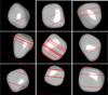 |
Fig. A.1 (275) Sapientia ADAM solution pole 2, shown with occultation chords used to construct the model. Occultation events are the same as in Fig. 4. |
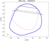 |
Fig. A.2 (286) Iclea model fit to occultation chords. Pole 2 (dashed contour) is rejected as inconsistent with all previous size determinations. |
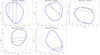 |
Fig. A.3 (326) Tamara model fit to occultation chords. Pole 1 is preferred (solid contour). |
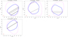 |
Fig. A.4 (412) Elisabetha model fit to occultation chords. Pole 2 is preferred (solid contour). |
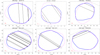 |
Fig. A.5 (426) Hippo model fit to occultation chords. Pole 2 is preferred (solid contour). |
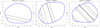 |
Fig. A.6 (439) Ohio model fit to occultation chords. |
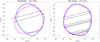 |
Fig. A.7 (464) Megaira model fit to occultation chords: pole 1 (blue), and pole 2 (magenta). |
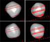 |
Fig. A.8 (464) Megaira ADAM solution pole 1 (top row), pole 2 (bottom row), shown with occultation chords used to construct the models. Occultation events same as in Fig. A.7. |
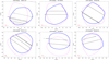 |
Fig. A.9 (476) Hedwig model fit to occultation chords. Pole 1 is preferred (solid contour). |
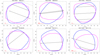 |
Fig. A.10 (524) Fidelio model fit to occultation chords. Pole 2 is preferred (blue contour). |
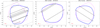 |
Fig. A.11 (530) Turandot model fit to occultation chords. Pole 2 is preferred (solid contour). |
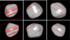 |
Fig. A.12 (530) Turandot ADAM solution pole 1 (top row), pole 2 (bottom row), shown with occultation chords used to construct the models. Occultation events same as in Fig. A.11. |
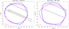 |
Fig. A.13 (551) Ortrud model fit to occultation chords: pole 1 (blue), and pole 2 (magenta). |
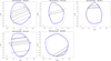 |
Fig. A.14 (566) Stereoskopia model fit to occultation chords. Pole 1 is preferred (solid contour). |
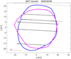 |
Fig. A.15 (657) Gunlod model fit to occultation chords. Pole 2 is preferred (blue contour). |
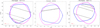 |
Fig. A.16 (738) Alagasta model fit to occultation chords: pole 2 (blue), and pole 1 (magenta). |
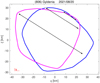 |
Fig. A.17 (806) Gyldenia model fit to occultation chords: pole 1 (blue), and pole 2 (magenta). |
Appendix B Observing campaign details
This section contains summarised details of all time-series observations used for the modelling (Table B.1), and the list of stellar occultation event observers and sites (Table B.2).
Details of all photometric observations for light curves: observing dates, number of light curves, range of ecliptic longitudes of the target, and sun-target-observer phase angles, observer name (or paper citation in case of published data), and the observing site. Some data come from robotic telescopes, in which case there is no observer specified. For data from the TESS spacecraft, Nic denotes the number of days of continuous observations. CSSS stands for Center for Solar System Studies, CTIO - Cerro Tololo Interamerican Observatory, e-EyE - Entre Encinas y Estrellas, ESO - European Southern Observatory, OASI - Observatorio Astronômico do Sertão de Itaparica, ORM - Roque de los Muchachos Observatory, OT - Observatorio del Teide, and SOAO - Sobaeksan Optical Astronomy Observatory.
List of stellar occultation observers and locations of their observing sites. Source: Occult programme.
Appendix C Light curves
Composite light curves presenting new data for target asteroids (Figures C.1 – C.77).
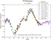 |
Fig. C.1 Composite light curve of (70) Panopaea from the years 2016-2017. |
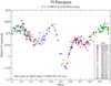 |
Fig. C.2 Composite light curve of (70) Panopaea from the year 2018. |
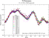 |
Fig. C.3 Composite light curve of (70) Panopaea from the year 2018 observed by TESS spacecraft. |
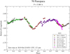 |
Fig. C.4 Composite light curve of (70) Panopaea from the year 2019. |
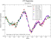 |
Fig. C.5 Composite light curve of (275) Sapientia from the years 2016-2017. |
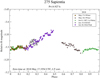 |
Fig. C.6 Composite light curve of (275) Sapientia from the year 2018. |
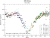 |
Fig. C.7 Composite light curve of (286) Iclea from the year 2007. |
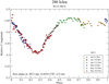 |
Fig. C.8 Composite light curve of (286) Iclea from the year 2013. |
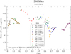 |
Fig. C.9 Composite light curve of (286) Iclea from the year 2014. |
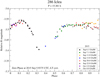 |
Fig. C.10 Composite light curve of (286) Iclea from the year 2015. |
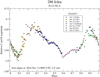 |
Fig. C.11 Composite light curve of (286) Iclea from the years 2016-2017. |
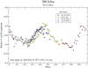 |
Fig. C.12 Composite light curve of (286) Iclea from the years 2017-2018. |
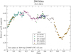 |
Fig. C.13 Composite light curve of (286) Iclea from the year 2019. |
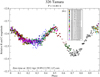 |
Fig. C.14 Composite light curve of (326) Tamara from the year 2012. |
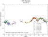 |
Fig. C.15 Composite light curve of (326) Tamara from the year 2015. |
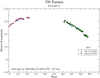 |
Fig. C.16 Composite light curve of (326) Tamara from March 2016. |
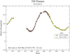 |
Fig. C.17 Composite light curve of (326) Tamara August-September 2016. |
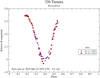 |
Fig. C.18 Composite light curve of (326) Tamara from October 2016. Data in 2016 were gathered in greatly varied phase angles and ecliptic longitudes, preventing the creation of one composite light curve (see Fig. C.16, and C.17). |
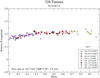 |
Fig. C.19 Composite light curve of (326) Tamara from the year 2017. |
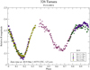 |
Fig. C.20 Composite light curve of (326) Tamara from the year 2019. |
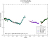 |
Fig. C.21 Composite light curve of (412) Elisabetha from the year 2016. |
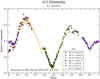 |
Fig. C.22 Composite light curve of (412) Elisabetha from the year 2017. |
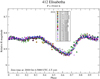 |
Fig. C.23 Composite light curve of (412) Elisabetha from the year 2018. |
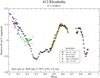 |
Fig. C.24 Composite light curve of (412) Elisabetha from the years 2019-2020. |
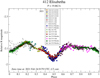 |
Fig. C.25 Composite light curve of (412) Elisabetha from the year 2021. |
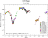 |
Fig. C.26 Composite light curve of (426) Hippo from the year 2015. |
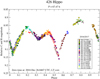 |
Fig. C.27 Composite light curve of (426) Hippo from the years 2016-2017. |
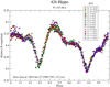 |
Fig. C.28 Composite light curve of (426) Hippo from the year 2019 observed by TESS spacecraft. |
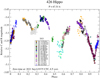 |
Fig. C.29 Composite light curve of (426) Hippo from the year 2021. |
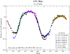 |
Fig. C.30 Composite light curve of (439) Ohio from the years 2015-2016. |
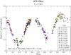 |
Fig. C.31 Composite light curve of (439) Ohio from the year 2018. |
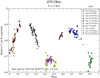 |
Fig. C.32 Composite light curve of (439) Ohio from the year 2019. |
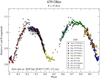 |
Fig. C.33 Composite light curve of (439) Ohio from the year 2020. |
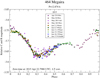 |
Fig. C.34 Composite light curve of (464) Megaira from the year 2015. |
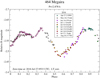 |
Fig. C.35 Composite light curve of (464) Megaira from the year 2016. |
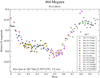 |
Fig. C.36 Composite light curve of (464) Megaira from the year 2017. |
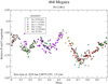 |
Fig. C.37 Composite light curve of (464) Megaira from the years 2018-2019. |
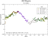 |
Fig. C.38 Composite light curve of (464) Megaira from the year 2020. |
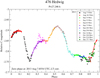 |
Fig. C.39 Composite light curve of (476) Hedwig from the year 2013. |
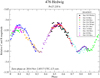 |
Fig. C.40 Composite light curve of (476) Hedwig from the years 2014-2015. |
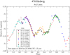 |
Fig. C.41 Composite light curve of (476) Hedwig from the year 2016. |
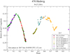 |
Fig. C.42 Composite light curve of (476) Hedwig from the year 2017. |
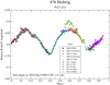 |
Fig. C.43 Composite light curve of (476) Hedwig from the year 2018. |
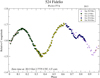 |
Fig. C.44 Composite light curve of (524) Fidelio from the year 2013. |
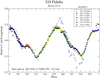 |
Fig. C.45 Composite light curve of (524) Fidelio from the years 2014-2015. |
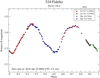 |
Fig. C.46 Composite light curve of (524) Fidelio from the year 2016. |
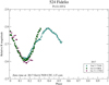 |
Fig. C.47 Composite light curve of (524) Fidelio from the year 2017. |
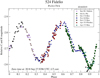 |
Fig. C.48 Composite light curve of (524) Fidelio from the years 2018-2019. |
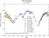 |
Fig. C.49 Composite light curve of (530) Turandot from the years 2015-2016. |
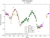 |
Fig. C.50 Composite light curve of (530) Turandot from the year 2016. |
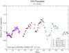 |
Fig. C.51 Composite light curve of (530) Turandot from the year 2018. |
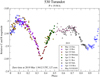 |
Fig. C.52 Composite light curve of (530) Turandot from the year 2019. |
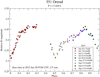 |
Fig. C.53 Composite light curve of (551) Ortrud from the year 2015. |
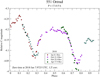 |
Fig. C.54 Composite light curve of (551) Ortrud from the year 2018. |
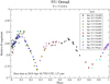 |
Fig. C.55 Composite light curve of (551) Ortrud from the year 2019. |
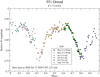 |
Fig. C.56 Composite light curve of (551) Ortrud from the year 2020. |
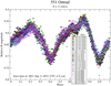 |
Fig. C.57 Composite light curve of (551) Ortrud from the year 2021, observed mainly from TESS spacecraft. |
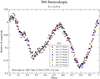 |
Fig. C.58 Composite light curve of (566) Stereoskopia from the year 2017, observed by Kepler mission. |
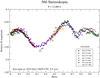 |
Fig. C.59 Composite light curve of (566) Stereoskopia from the years 2019-2020. |
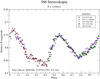 |
Fig. C.60 Composite light curve of (566) Stereoskopia from the years 2020-2021. |
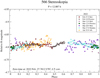 |
Fig. C.61 Composite light curve of (566) Stereoskopia from the year 2022. |
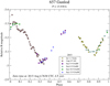 |
Fig. C.62 Composite light curve of (657) Gunlod fiOm the year 2015. |
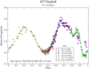 |
Fig. C.63 Composite light curve of (657) Gunlod from the year 2016, obsbrved mainly from TESS spacecraft. |
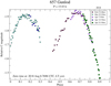 |
Fig. C.64 Composite light curve of (657) Gunlod from the year 2018, observed by Kepler mission. |
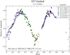 |
Fig. C.65 Composite light curve of (657) (Gunlod drom the eear 2020. |
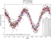 |
Fig. C.66 Composite light curve of (657) Gunlod from the year 2021 from TESS spacecraft. |
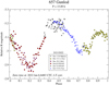 |
Fig. C.67 Composite light curve of (657) Gunlod from the years 2021–2022. Given the different character of the light curve caused by slightly different viewing geometry, it could not be folded with the light curve from Fig. C.66. |
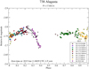 |
Fig. C.68 Composite light curve of (738) Alagasta from the year 2015. |
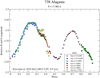 |
Fig. C.69 Composite light curve of (738) Alagasta from the year 2016. |
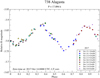 |
Fig. C.70 Composite light curve of (738) Alagasta from the year 2017. |
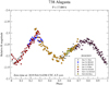 |
Fig. C.71 Composite light curve of (738) Alagasta from the years 2018-2019. |
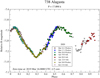 |
Fig. C.72 Composite light curve of (738) Alagasta from the year 2020. |
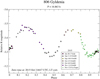 |
Fig. C.73 Composite light curve of (806) Gyldenia from the year 2015. |
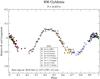 |
Fig. C.74 Composite light curve of (806) Gyldenia from the year 2016. |
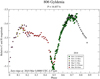 |
Fig. C.75 Composite light curve of (806) Gyldenia from the year 2018. |
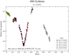 |
Fig. C.76 Composite light curve of (806) Gyldenia from the year 2020. |
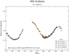 |
Fig. C.77 Composite light curve of (806) Gyldenia from the year 2021. |
References
- Alí-Lagoa, V., Müller, T. G., Usui, F., & Hasegawa, S. 2018, A&A, 612, A85 [NASA ADS] [CrossRef] [EDP Sciences] [Google Scholar]
- Alkema, M. S. 2013, Minor Planet Bull., 40, 215 [NASA ADS] [Google Scholar]
- Binzel, R. P. 1987, Icarus, 72, 135 [Google Scholar]
- Binzel, R. P., & Sauter, L. M. 1992, Icarus, 95, 222 [NASA ADS] [CrossRef] [Google Scholar]
- Brož, M., Morbidelli, A., Bottke, W. F., et al. 2013, A&A, 551, A117 Buie, M. W., & Keller, J. M. 2016, AJ, 151, 73 [Google Scholar]
- Carry, B. 2012, Planet. Space Sci., 73, 98 [CrossRef] [Google Scholar]
- Delbo’, M., Mueller, M., Emery, J. P., Rozitis, B., & Capria, M. T. 2015, Asteroid Thermophysical Modeling, 107 [Google Scholar]
- Denchev, P. 2000, Planet. Space Sci., 48, 987 [NASA ADS] [CrossRef] [Google Scholar]
- di Martino, M., Dotto, E., Cellino, A., Barucci, M. A., & Fulchignoni, M. 1995, A&AS, 112, 1 [NASA ADS] [Google Scholar]
- Ďurech, J., Sidorin, V., & Kaasalainen, M. 2010, A&A, 513, A46 [Google Scholar]
- Ďurech, J., Kaasalainen, M., Herald, D., et al. 2011, Icarus, 214, 652 [Google Scholar]
- Ďurech, J., Hanuš, J., & Alí-Lagoa, V. 2018, A&A, 617, A57 [NASA ADS] [CrossRef] [EDP Sciences] [Google Scholar]
- Ďurech, J., Hanuš, J., & Vančo, R. 2019, A&A, 631, A2 [Google Scholar]
- Ďurech, J., Tonry, J., Erasmus, N., et al. 2020, A&A, 643, A59 [NASA ADS] [CrossRef] [EDP Sciences] [Google Scholar]
- Ďurech, J., Vokrouhlický, D., Pravec, P., et al. 2022, A&A, 657, A5 [NASA ADS] [CrossRef] [EDP Sciences] [Google Scholar]
- Gaia Collaboration (Brown, A. G. A., et al.) 2021, A&A, 649, A1 [NASA ADS] [CrossRef] [EDP Sciences] [Google Scholar]
- Gault, D., Nosworthy, P., Nolthenius, R., Bender, K., & Herald, D. 2022, Minor Planet Bull., 49, 3 [Google Scholar]
- Hainaut-Rouelle, M. C., Hainaut, O. R., & Detal, A. 1995, A&AS, 112, 125 [NASA ADS] [Google Scholar]
- Hanuš, J., Ďurech, J., Oszkiewicz, D. A., et al. 2016, A&A, 586, A108 [NASA ADS] [CrossRef] [EDP Sciences] [Google Scholar]
- Hanuš, J., Delbo’, M., Alí-Lagoa, V., et al. 2018, Icarus, 299, 84 [CrossRef] [Google Scholar]
- Hanuš, J., Pejcha, O., Shappee, B. J., et al. 2021, A&A, 654, A48 [NASA ADS] [CrossRef] [EDP Sciences] [Google Scholar]
- Harris, A. W. 1998, Icarus, 131, 291 [Google Scholar]
- Harris, A. W., & Drube, L. 2016, ApJ, 832, 127 [NASA ADS] [CrossRef] [Google Scholar]
- Harris, A. W., & Drube, L. 2020, ApJ, 901, 140 [NASA ADS] [CrossRef] [Google Scholar]
- Harris, A. W., & Harris, A. W. 1997, Icarus, 126, 450 [Google Scholar]
- Harris, A. W., & Lagerros, J. S. V. 2002, in Asteroids III (Tucson: University of Arizona Press), 205 [Google Scholar]
- Harris, A. W., & Young, J. W. 1989, Icarus, 81, 314 [NASA ADS] [CrossRef] [Google Scholar]
- Harris, A. W., Young, J. W., Dockweiler, T., et al. 1992, Icarus, 95, 115 [NASA ADS] [CrossRef] [Google Scholar]
- Herald, D., Frappa, E., Gault, D., et al. 2019, Asteroid Occultations V3.0, NASA Planetary Data System [Google Scholar]
- Herald, D., Gault, D., Anderson, R., et al. 2020, MNRAS, 499, 4570 [Google Scholar]
- Higgins, D. 2011, Minor Planet Bull., 38, 41 [NASA ADS] [Google Scholar]
- Kaasalainen, M., & Torppa, J. 2001, Icarus, 153, 24 [NASA ADS] [CrossRef] [Google Scholar]
- Kaasalainen, M., & Lamberg, L. 2006, Inverse Probl., 22, 749 [Google Scholar]
- Kaasalainen, M., Torppa, J., & Muinonen, K. 2001, Icarus, 153, 37 [NASA ADS] [CrossRef] [Google Scholar]
- Kalup, C. E., Molnár, L., Kiss, C., et al. 2021, ApJS, 254, 7 [NASA ADS] [CrossRef] [Google Scholar]
- Koff, R. A. 2006, Minor Planet Bull., 33, 31 [NASA ADS] [Google Scholar]
- Lagerkvist, C. I., Hahn, G., Magnusson, P., & Rickman, H. 1987, A&AS, 70, 21 [NASA ADS] [Google Scholar]
- Lagerkvist, C. I., Magnusson, P., Debehogne, H., et al. 1992, A&AS, 95, 461 [NASA ADS] [Google Scholar]
- Marciniak, A., Pilcher, F., Oszkiewicz, D., et al. 2015, Planet. Space Sci., 118, 256 [NASA ADS] [CrossRef] [Google Scholar]
- Marciniak, A., Pilcher, F., Oszkiewicz, D., et al. 2016, in 37th Meeting of the Polish Astronomical Society, 3, eds. A. Rozanska, & M. Bejger, 84 [Google Scholar]
- Marciniak, A., Bartczak, P., Müller, T., et al. 2018, A&A, 610, A7 [NASA ADS] [CrossRef] [EDP Sciences] [Google Scholar]
- Marciniak, A., Alí-Lagoa, V., Müller, T. G., et al. 2019, A&A, 625, A139 [NASA ADS] [CrossRef] [EDP Sciences] [Google Scholar]
- Marciniak, A., Ďurech, J., Alí-Lagoa, V., et al. 2021, A&A, 654, A87 [NASA ADS] [CrossRef] [EDP Sciences] [Google Scholar]
- Masiero, J. R., Mainzer, A. K., Grav, T., et al. 2011, ApJ, 741, 68 [Google Scholar]
- Masiero, J. R., Mainzer, A. K., Grav, T., et al. 2012, ApJ, 759, L8 [NASA ADS] [CrossRef] [Google Scholar]
- Masiero, J. R., Nugent, C., Mainzer, A. K., et al. 2017, AJ, 154, 168 [NASA ADS] [CrossRef] [Google Scholar]
- Masiero, J. R., Mainzer, A. K., Bauer, J. M., et al. 2020, Planet. Sci. J., 1, 5 [NASA ADS] [CrossRef] [Google Scholar]
- Masiero, J. R., Mainzer, A. K., Bauer, J. M., et al. 2021, Planet. Sci. J., 2, 162 [CrossRef] [Google Scholar]
- Mohamed, R. A., Krugly, Y. N., & Lupishko, D. F. 1995, AJ, 109, 1877 [NASA ADS] [CrossRef] [Google Scholar]
- Molnár, L., Pál, A., Sârneczky, K., et al. 2018, ApJS, 234, 37 [CrossRef] [Google Scholar]
- Morbidelli, A., Bottke, W. F., Nesvorný, D., & Levison, H. F. 2009, Icarus, 204, 558 [Google Scholar]
- Nugent, C. R., Mainzer, A., Bauer, J., et al. 2016, AJ, 152, 63 [Google Scholar]
- Ortiz, J. L., Santos-Sanz, P., Sicardy, B., et al. 2017, Nature, 550, 219 [NASA ADS] [CrossRef] [Google Scholar]
- Pál, A., Szakáts, R., Kiss, C., et al. 2020, ApJS, 247, 26 [CrossRef] [Google Scholar]
- Pilcher, F. 2014, Minor Planet Bull., 41, 250 [NASA ADS] [Google Scholar]
- Pilcher, F. 2015, Minor Planet Bull., 42, 38 [NASA ADS] [Google Scholar]
- Pilcher, F. 2016, Minor Planet Bull., 43, 135 [NASA ADS] [Google Scholar]
- Pilcher, F. 2019, Minor Planet Bull., 46, 360 [NASA ADS] [Google Scholar]
- Pilcher, F., Benishek, V., Bonamico, R., et al. 2021, Minor Planet Bull., 48, 4 [NASA ADS] [Google Scholar]
- Polakis, T. 2021a, Minor Planet Bull., 48, 394 [NASA ADS] [Google Scholar]
- Polakis, T. 2021b, Minor Planet Bull., 48, 23 [NASA ADS] [Google Scholar]
- Raskin, G., Bloemen, S., Morren, J., et al. 2013, A&A, 559, A26 [NASA ADS] [CrossRef] [EDP Sciences] [Google Scholar]
- Ryan, E. L., & Woodward, C. E. 2010, AJ, 140, 933 [NASA ADS] [CrossRef] [Google Scholar]
- Schober, H. J., & Schroll, A. 1985, A&AS, 62, 187 [NASA ADS] [Google Scholar]
- Schroll, A., & Schober, H. J. 1983, A&AS, 53, 77 [NASA ADS] [Google Scholar]
- Stephens, R. D. 2012, Minor Planet Bull., 39, 226 [NASA ADS] [Google Scholar]
- Tanga, P., Delbo, M., & Gerakis, J. 2013, in AAS/Division for Planetary Sciences Meeting Abstracts, 45, 208.29 [Google Scholar]
- Tanga, P., Pauwels, T., Mignard, F., et al. 2022, A&A, 674, A12 [Google Scholar]
- Vernazza, P., Ferrais, M., Jorda, L., et al. 2021, A&A, 654, A56 [NASA ADS] [CrossRef] [EDP Sciences] [Google Scholar]
- Viikinkoski, M., Kaasalainen, M., & Ďurech, J. 2015, A&A, 576, A8 [NASA ADS] [CrossRef] [EDP Sciences] [Google Scholar]
- Vokrouhlický, D., Brož, M., Bottke, W. F., Nesvorný, D., & Morbidelli, A. 2006, Icarus, 182, 118 [Google Scholar]
- Warner, B. D. 2007, Minor Planet Bull., 34, 72 [NASA ADS] [Google Scholar]
- Warner, B. D., Harris, A. W., & Pravec, P. 2009, Icarus, 202, 134 [NASA ADS] [CrossRef] [Google Scholar]
- Waszczak, A., Chang, C.-K., Ofek, E. O., et al. 2015, AJ, 150, 75 [NASA ADS] [CrossRef] [Google Scholar]
- Wright, E. L., Eisenhardt, P. R. M., Mainzer, A. K., et al. 2010, AJ, 140, 1868 [Google Scholar]
All Tables
Details of all photometric observations for light curves: observing dates, number of light curves, range of ecliptic longitudes of the target, and sun-target-observer phase angles, observer name (or paper citation in case of published data), and the observing site. Some data come from robotic telescopes, in which case there is no observer specified. For data from the TESS spacecraft, Nic denotes the number of days of continuous observations. CSSS stands for Center for Solar System Studies, CTIO - Cerro Tololo Interamerican Observatory, e-EyE - Entre Encinas y Estrellas, ESO - European Southern Observatory, OASI - Observatorio Astronômico do Sertão de Itaparica, ORM - Roque de los Muchachos Observatory, OT - Observatorio del Teide, and SOAO - Sobaeksan Optical Astronomy Observatory.
List of stellar occultation observers and locations of their observing sites. Source: Occult programme.
All Figures
|
Fig. 1 Two versions of shape model 2 for (566) Stereoskopia: without shape regularisation (top) and with regularisation applied (bottom), using the same starting parameters otherwise. The three views show, from left to right: two equatorial views separated by 90°in phase, and the pole-on view. We note that the pole-on silhouettes generally agree between two versions of the shape model, as it is the equatorial cross-section that most effectively influences the light curves. |
| In the text | |
|
Fig. 2 Two versions of shape model 2 for (412) Elisabetha. The high-regularisation model (bottom) still fits the light curves on formally acceptable level, but is unrealistically flat. See Sect. 4 for discussion. |
| In the text | |
|
Fig. 3 (70) Panopaea model fit to occultation chords shown in the fundamental plane. North is up and west is right. Dashed lines mark visual observations, as opposed to video or photoelectric ones marked with solid lines. Grey segments correspond to timing uncertainties. Blue contour: Instantaneous silhouette of shape model 1 (see Table 1). Magenta: Same but for model 2. In this case, occultations show no preference for any of the models. |
| In the text | |
|
Fig. 4 (275) Sapientia model fit to occultation chords. Here, model 2 is preferred (blue solid contour). |
| In the text | |
|
Fig. 5 (275) Sapientia, ADAM solution pole 1, shown with occultation chords used to construct the model. Occultation events are the same as in Fig. 4. |
| In the text | |
|
Fig. A.1 (275) Sapientia ADAM solution pole 2, shown with occultation chords used to construct the model. Occultation events are the same as in Fig. 4. |
| In the text | |
|
Fig. A.2 (286) Iclea model fit to occultation chords. Pole 2 (dashed contour) is rejected as inconsistent with all previous size determinations. |
| In the text | |
|
Fig. A.3 (326) Tamara model fit to occultation chords. Pole 1 is preferred (solid contour). |
| In the text | |
|
Fig. A.4 (412) Elisabetha model fit to occultation chords. Pole 2 is preferred (solid contour). |
| In the text | |
|
Fig. A.5 (426) Hippo model fit to occultation chords. Pole 2 is preferred (solid contour). |
| In the text | |
|
Fig. A.6 (439) Ohio model fit to occultation chords. |
| In the text | |
|
Fig. A.7 (464) Megaira model fit to occultation chords: pole 1 (blue), and pole 2 (magenta). |
| In the text | |
|
Fig. A.8 (464) Megaira ADAM solution pole 1 (top row), pole 2 (bottom row), shown with occultation chords used to construct the models. Occultation events same as in Fig. A.7. |
| In the text | |
|
Fig. A.9 (476) Hedwig model fit to occultation chords. Pole 1 is preferred (solid contour). |
| In the text | |
|
Fig. A.10 (524) Fidelio model fit to occultation chords. Pole 2 is preferred (blue contour). |
| In the text | |
|
Fig. A.11 (530) Turandot model fit to occultation chords. Pole 2 is preferred (solid contour). |
| In the text | |
|
Fig. A.12 (530) Turandot ADAM solution pole 1 (top row), pole 2 (bottom row), shown with occultation chords used to construct the models. Occultation events same as in Fig. A.11. |
| In the text | |
|
Fig. A.13 (551) Ortrud model fit to occultation chords: pole 1 (blue), and pole 2 (magenta). |
| In the text | |
|
Fig. A.14 (566) Stereoskopia model fit to occultation chords. Pole 1 is preferred (solid contour). |
| In the text | |
|
Fig. A.15 (657) Gunlod model fit to occultation chords. Pole 2 is preferred (blue contour). |
| In the text | |
|
Fig. A.16 (738) Alagasta model fit to occultation chords: pole 2 (blue), and pole 1 (magenta). |
| In the text | |
|
Fig. A.17 (806) Gyldenia model fit to occultation chords: pole 1 (blue), and pole 2 (magenta). |
| In the text | |
|
Fig. C.1 Composite light curve of (70) Panopaea from the years 2016-2017. |
| In the text | |
|
Fig. C.2 Composite light curve of (70) Panopaea from the year 2018. |
| In the text | |
|
Fig. C.3 Composite light curve of (70) Panopaea from the year 2018 observed by TESS spacecraft. |
| In the text | |
|
Fig. C.4 Composite light curve of (70) Panopaea from the year 2019. |
| In the text | |
|
Fig. C.5 Composite light curve of (275) Sapientia from the years 2016-2017. |
| In the text | |
|
Fig. C.6 Composite light curve of (275) Sapientia from the year 2018. |
| In the text | |
|
Fig. C.7 Composite light curve of (286) Iclea from the year 2007. |
| In the text | |
|
Fig. C.8 Composite light curve of (286) Iclea from the year 2013. |
| In the text | |
|
Fig. C.9 Composite light curve of (286) Iclea from the year 2014. |
| In the text | |
|
Fig. C.10 Composite light curve of (286) Iclea from the year 2015. |
| In the text | |
|
Fig. C.11 Composite light curve of (286) Iclea from the years 2016-2017. |
| In the text | |
|
Fig. C.12 Composite light curve of (286) Iclea from the years 2017-2018. |
| In the text | |
|
Fig. C.13 Composite light curve of (286) Iclea from the year 2019. |
| In the text | |
|
Fig. C.14 Composite light curve of (326) Tamara from the year 2012. |
| In the text | |
|
Fig. C.15 Composite light curve of (326) Tamara from the year 2015. |
| In the text | |
|
Fig. C.16 Composite light curve of (326) Tamara from March 2016. |
| In the text | |
|
Fig. C.17 Composite light curve of (326) Tamara August-September 2016. |
| In the text | |
|
Fig. C.18 Composite light curve of (326) Tamara from October 2016. Data in 2016 were gathered in greatly varied phase angles and ecliptic longitudes, preventing the creation of one composite light curve (see Fig. C.16, and C.17). |
| In the text | |
|
Fig. C.19 Composite light curve of (326) Tamara from the year 2017. |
| In the text | |
|
Fig. C.20 Composite light curve of (326) Tamara from the year 2019. |
| In the text | |
|
Fig. C.21 Composite light curve of (412) Elisabetha from the year 2016. |
| In the text | |
|
Fig. C.22 Composite light curve of (412) Elisabetha from the year 2017. |
| In the text | |
|
Fig. C.23 Composite light curve of (412) Elisabetha from the year 2018. |
| In the text | |
|
Fig. C.24 Composite light curve of (412) Elisabetha from the years 2019-2020. |
| In the text | |
|
Fig. C.25 Composite light curve of (412) Elisabetha from the year 2021. |
| In the text | |
|
Fig. C.26 Composite light curve of (426) Hippo from the year 2015. |
| In the text | |
|
Fig. C.27 Composite light curve of (426) Hippo from the years 2016-2017. |
| In the text | |
|
Fig. C.28 Composite light curve of (426) Hippo from the year 2019 observed by TESS spacecraft. |
| In the text | |
|
Fig. C.29 Composite light curve of (426) Hippo from the year 2021. |
| In the text | |
|
Fig. C.30 Composite light curve of (439) Ohio from the years 2015-2016. |
| In the text | |
|
Fig. C.31 Composite light curve of (439) Ohio from the year 2018. |
| In the text | |
|
Fig. C.32 Composite light curve of (439) Ohio from the year 2019. |
| In the text | |
|
Fig. C.33 Composite light curve of (439) Ohio from the year 2020. |
| In the text | |
|
Fig. C.34 Composite light curve of (464) Megaira from the year 2015. |
| In the text | |
|
Fig. C.35 Composite light curve of (464) Megaira from the year 2016. |
| In the text | |
|
Fig. C.36 Composite light curve of (464) Megaira from the year 2017. |
| In the text | |
|
Fig. C.37 Composite light curve of (464) Megaira from the years 2018-2019. |
| In the text | |
|
Fig. C.38 Composite light curve of (464) Megaira from the year 2020. |
| In the text | |
|
Fig. C.39 Composite light curve of (476) Hedwig from the year 2013. |
| In the text | |
|
Fig. C.40 Composite light curve of (476) Hedwig from the years 2014-2015. |
| In the text | |
|
Fig. C.41 Composite light curve of (476) Hedwig from the year 2016. |
| In the text | |
|
Fig. C.42 Composite light curve of (476) Hedwig from the year 2017. |
| In the text | |
|
Fig. C.43 Composite light curve of (476) Hedwig from the year 2018. |
| In the text | |
|
Fig. C.44 Composite light curve of (524) Fidelio from the year 2013. |
| In the text | |
|
Fig. C.45 Composite light curve of (524) Fidelio from the years 2014-2015. |
| In the text | |
|
Fig. C.46 Composite light curve of (524) Fidelio from the year 2016. |
| In the text | |
|
Fig. C.47 Composite light curve of (524) Fidelio from the year 2017. |
| In the text | |
|
Fig. C.48 Composite light curve of (524) Fidelio from the years 2018-2019. |
| In the text | |
|
Fig. C.49 Composite light curve of (530) Turandot from the years 2015-2016. |
| In the text | |
|
Fig. C.50 Composite light curve of (530) Turandot from the year 2016. |
| In the text | |
|
Fig. C.51 Composite light curve of (530) Turandot from the year 2018. |
| In the text | |
|
Fig. C.52 Composite light curve of (530) Turandot from the year 2019. |
| In the text | |
|
Fig. C.53 Composite light curve of (551) Ortrud from the year 2015. |
| In the text | |
|
Fig. C.54 Composite light curve of (551) Ortrud from the year 2018. |
| In the text | |
|
Fig. C.55 Composite light curve of (551) Ortrud from the year 2019. |
| In the text | |
|
Fig. C.56 Composite light curve of (551) Ortrud from the year 2020. |
| In the text | |
|
Fig. C.57 Composite light curve of (551) Ortrud from the year 2021, observed mainly from TESS spacecraft. |
| In the text | |
|
Fig. C.58 Composite light curve of (566) Stereoskopia from the year 2017, observed by Kepler mission. |
| In the text | |
|
Fig. C.59 Composite light curve of (566) Stereoskopia from the years 2019-2020. |
| In the text | |
|
Fig. C.60 Composite light curve of (566) Stereoskopia from the years 2020-2021. |
| In the text | |
|
Fig. C.61 Composite light curve of (566) Stereoskopia from the year 2022. |
| In the text | |
|
Fig. C.62 Composite light curve of (657) Gunlod fiOm the year 2015. |
| In the text | |
|
Fig. C.63 Composite light curve of (657) Gunlod from the year 2016, obsbrved mainly from TESS spacecraft. |
| In the text | |
|
Fig. C.64 Composite light curve of (657) Gunlod from the year 2018, observed by Kepler mission. |
| In the text | |
|
Fig. C.65 Composite light curve of (657) (Gunlod drom the eear 2020. |
| In the text | |
|
Fig. C.66 Composite light curve of (657) Gunlod from the year 2021 from TESS spacecraft. |
| In the text | |
|
Fig. C.67 Composite light curve of (657) Gunlod from the years 2021–2022. Given the different character of the light curve caused by slightly different viewing geometry, it could not be folded with the light curve from Fig. C.66. |
| In the text | |
|
Fig. C.68 Composite light curve of (738) Alagasta from the year 2015. |
| In the text | |
|
Fig. C.69 Composite light curve of (738) Alagasta from the year 2016. |
| In the text | |
|
Fig. C.70 Composite light curve of (738) Alagasta from the year 2017. |
| In the text | |
|
Fig. C.71 Composite light curve of (738) Alagasta from the years 2018-2019. |
| In the text | |
|
Fig. C.72 Composite light curve of (738) Alagasta from the year 2020. |
| In the text | |
|
Fig. C.73 Composite light curve of (806) Gyldenia from the year 2015. |
| In the text | |
|
Fig. C.74 Composite light curve of (806) Gyldenia from the year 2016. |
| In the text | |
|
Fig. C.75 Composite light curve of (806) Gyldenia from the year 2018. |
| In the text | |
|
Fig. C.76 Composite light curve of (806) Gyldenia from the year 2020. |
| In the text | |
|
Fig. C.77 Composite light curve of (806) Gyldenia from the year 2021. |
| In the text | |
Current usage metrics show cumulative count of Article Views (full-text article views including HTML views, PDF and ePub downloads, according to the available data) and Abstracts Views on Vision4Press platform.
Data correspond to usage on the plateform after 2015. The current usage metrics is available 48-96 hours after online publication and is updated daily on week days.
Initial download of the metrics may take a while.