| Issue |
A&A
Volume 693, January 2025
|
|
|---|---|---|
| Article Number | A96 | |
| Number of page(s) | 27 | |
| Section | Galactic structure, stellar clusters and populations | |
| DOI | https://doi.org/10.1051/0004-6361/202346654 | |
| Published online | 07 January 2025 | |
The NenuFAR Pulsar Blind Survey (NPBS): I. Survey overview, expectations, and first redetections
1
Laboratoire de Physique et Chimie de l’Environnement et de l’Espace (LPC2E) Université d’Orléans/CNRS,
Orléans,
France
2
Observatoire Radioastronomique de Nançay (ORN), Observatoire de Paris, Université PSL, Univ Orléans, CNRS,
18330
Nançay,
France
3
Laboratoire Univers et Théories LUTh, Observatoire de Paris, CNRS/INSU, Université Paris,
France
4
Institute of Radio Astronomy of NAS of Ukraine,
4 Mystetstv St.,
61002,
Kharkiv,
Ukraine
5
LESIA, Observatoire de Paris, Université PSL, Sorbonne Université, Université Paris Cité, CNRS,
92190
Meudon,
France
6
Max-Planck-Institut für Radioastronomie,
Auf dem Hügel 69,
53121
Bonn,
Germany
7
ASTRON, the Netherlands Institute for Radio Astronomy,
Oude Hoogeveensedijk 4,
7991 PD
Dwingeloo,
The Netherlands
8
E.A. Milne Centre for Astrophysics, University of Hull,
Cottingham Road,
Kingston-upon-Hull,
HU6 7RX,
UK
9
Centre of Excellence for Data Science, Artificial Intelligence and Modelling (DAIM), University of Hull,
Cottingham Road,
Kingston-upon-Hull,
HU6 7RX,
UK
10
INAF-Osservatorio Astronomico di Cagliari,
via della Scienza 5,
09047
Selargius,
Italy
11
Université Paris Cité and Université Paris Saclay, CEA, CNRS, AIM,
91190
Gif-sur-Yvette,
France
★ Corresponding author; This email address is being protected from spambots. You need JavaScript enabled to view it.
Received:
14
April
2023
Accepted:
3
October
2024
Abstract
The NenuFAR Pulsar Blind Survey (NPBS) is an all-sky survey, searching for pulsars at radio frequencies below 85 MHz with the NenuFAR radio telescope. Taking into account the turnover at low frequencies in the pulsar spectra and the widening of their emission cone towards low frequencies, we expect approximately 8–20 not already discovered pulsars to be detectable by this survey, most of which are likely to be non-standard pulsars or pulsars in unusual parts of the P − Ṗ diagram (such as, e.g. slow pulsars). According to our simulations, we expect the discovered pulsars to feature spectra with spectral indices ≲ −3.2 and low turnover frequencies <<85 MHz. Conversely, a non-detection would give valuable clues as to the population of pulsars in this region of the parameter space. The current first stage of the survey observes declinations above 39° in the frequency range 39–76 MHz. A frequency-averaged sky coverage of 98% is reached by observing 7692 pointings of about 1.5° of radius in 27 min each. The observing programme started in August 2020, and is expected to be completed during 2024. Approximately a third of the data are currently being processed using a search pipeline based on PRESTO with some adaptations to low frequencies. Because of the high scatter broadening and the coarse time resolution, the NPBS searches for pulsars with periods from 30 ms to 30 s and dispersion measures (DMs) between 1 and 70 pc cm−3. In the processed data, 24 known pulsars have been searched in order to verify the observing setup and the search pipeline. Seven of these pulsars have been detected, with DMs between 5 and 42 pc cm−3. The related candidates have periods between 40 ms to 3.5 s, including candidates corresponding to harmonics. Of the seven, six correspond to the most intense pulsars of the set. The last detection is presumably due to a beneficial effect of the scintillation. Based on the faintest detection, the expected minimum signal-to-noise ratio for detecting a pulsar is 4.8, corresponding to a minimum flux of 6.9 mJy in the coldest regions of the sky.
Key words: surveys / pulsars: general
© The Authors 2025
 Open Access article, published by EDP Sciences, under the terms of the Creative Commons Attribution License (https://creativecommons.org/licenses/by/4.0), which permits unrestricted use, distribution, and reproduction in any medium, provided the original work is properly cited.
This article is published in open access under the Subscribe to Open model. This email address is being protected from spambots. You need JavaScript enabled to view it. to support open access publication.
1 Introduction
Pulsars are astrophysical objects discovered in 1967 (Hewish et al. 1968). They were quickly related to supernova remnants and identified as rapidly rotating and magnetised neutron stars (Pacini 1968; Gold 1968). Pulsars are compact stars of about 1.4 M⊙ with a radius of about 13 km (Miller et al. 2019) and a rotating period typically between 1 ms and a few tens of seconds. Goldreich & Julian (1969) showed that their high magnetic fields (from 108 to 1014 G) accelerate the surrounded plasma to produce a radio emission tangentially to the field lines. This results in a radio emission cone rotating around the star’s rotation axis, which can be detected when it crosses the line of sight of Earth.
A pulse profile, with a shape and features particular to the pulsar, can be related to the geometry of the radio beam: either following a more or less complex emission cone Rankin (1993, 2022), or following patchy emission (Manchester et al. 2010; Desvignes et al. 2019). Pulsars can be used to study the highly dense matter (Zhu et al. 2023) or highly magnetised environments (Pétri 2022). In particular, in the case of binary systems (or triple or more in the case of orbiting planets), they can also be used to test the gravity theories (Della Monica et al. 2023). Finally, because of the dispersion of the radio emission in ionised environments, they are useful to probe the interstellar medium (ISM hereafter) (Cordes & Lazio 2003), the Solar System environment (Tiburzi et al. 2023), or the supernova remnants (Liu et al. 2023).
Although the first pulsars were discovered at low frequencies, primarily by the first Cambridge survey (Hewish et al. 1968; Cole & Pilkington 1968; Pilkington et al. 1968) which observed at 81.5 MHz, the vast majority of the currently known pulsars have been detected at higher frequencies, typically between 300 MHz and a few gigahertz. For the Northern Hemisphere, major surveys have been performed using the Green Bank telescope (such as the GBNCC, McEwen et al. 2020) and the Arecibo telescope (such as the PALFA, Lazarus et al. 2015). However, the most prolific surveys have been carried out in the Southern Hemisphere, with the second Molonglo survey (Manchester et al. 1978) in the 1970s, and several surveys using the Parkes telescope since the 1990s. In particular, the Parkes multi-beam pulsar survey (PMPS, Manchester et al. 2001) has discovered 834 pulsars. More recently, surveys using a new generation of radiotelescopes have been performed at diverse frequencies. In particular, the telescope FAST with its high sensitivity has discovered more than 200 pulsars since 2019 (GPPS, Han et al. 2021).
This article presents an overview of a pulse survey that started in 2020 using the phased array telescope NenuFAR (New extension in Nançay upgrading LOFAR, see Sect. 3.1). The Nen- uFAR Pulsar Blind Survey, hereafter refered to as NPBS, aims to search for pulsars at frequencies below 80 MHz (just below the lowest frequencies reached by the historical Cambridge pulsar surveys). Although the goal is to ultimately observe the entire northern sky (i.e. with a declination above 0°), the first stage presented here observes the northern polar cap above 39° of declination.
Few telescopes can observe pulsars at frequencies below 300 MHz. One can cite LOFAR (van Haarlem et al. 2013) observing between 10 and 240 MHz, the LWA (Ellingson et al. 2009) in a bandwidth similar to NenuFAR from 10 to 88 MHz, the MWA (Tingay et al. 2013) between 70 and 300 MHz, or UTR-2 (Zakharenko et al. 2005) observing at very-low frequencies from 10 to 30 MHz. Consequently, pulsar observations below 300 MHz are relatively uncommon, especially for a survey. According to the typical pulsar spectrum, it may indeed be easier to detect a pulsar at a high frequency, leading to a substantial number of pulsar surveys around 1.4 GHz. The NPBS is therefore motivated by the perspective to probe a part of the spectrum (below 100 MHz) rarely observed. Also, compared to the telescopes used for other surveys at frequencies below 100 MHz, NenuFAR is a more recent phased array telescope. It allows for a larger observing frequency bandwidth and a better sensitivity than previous surveys below 100 MHz.
The objective of the NPBS is to discover new pulsars that have not been detected at higher frequencies. Because of the typical pulsar spectrum and the fact that the entire sky was already observed by high-frequency surveys, we expect to primarily detect either non-standard pulsars with a steeper-than-average spectrum or standard pulsars with a wider emission cone at a low frequency. Detecting standard pulsars could provide information about the pulsar’s magnetosphere. On the other hand, detecting non-standard pulsars could indicate the existence of one or several new populations of pulsars. With such non-standard pulsars, we therefore expect to be able to explore sparsely populated regions of the P − Ṗ diagram (rotating period verses the period derivative of pulsars), in particular the region of slow pulsars close to the so-called death line of the pulsar phenomenon. Similarly, a non-detection with the NPBS would give valuable clues as to the population of pulsars in this region of the P − Ṗ parameter space.
These expectations are supported by the recent results of the LOTAAS survey (Sanidas et al. 2019), carried out at a central frequency of 135 MHz using LOFAR. The results of LOTAAS, leading to the discovery of 74 pulsars (Sanidas et al. 2019), are particularly relevant for NenuFAR because it is one of the lowest-frequency pulsar surveys from the last two decades. Looking at the period distribution of these discoveries, the majority of them are non-recycled and rotation-powered pulsars, proving there still remain pulsars that have not been discovered by high-frequency surveys.
Also, a significant number of pulsars discovered by LOTAAS are relatively slow pulsars with a rotation period of several seconds (see, e.g. Fig. 8 of Sanidas et al. 2019). Furthermore, one of the notable discoveries of LOTAAS was the pulsar J0250+5854 (Tan et al. 2018). With a rotation period of 23.535 s, it was the slowest known pulsar at the time of its discovery. Also, this discovery is interesting for low-frequency surveys because J0250+5854 presents a steep spectrum and is localised in the P − Ṗ diagram in a position below the death line of pulsars provided by some models.
The LOTAAS survey was performed for frequencies greater than those of the NPBS. On the other side, at even lower frequencies (16.5–33 MHz), a blind survey for pulsars and transients was carried out at UTR-2 (Vasylieva et al. 2014). While this survey did not discover new pulsars, it allowed for the re-detection and confirmation of the recently discovered pulsar J0240+62.
Radio observations below 100 MHz have to deal with several difficulties that strongly constrain the capacity to detect a pulsar. Firstly, three physical effects produced by the interstellar medium (ISM) can be noted. The first one is dispersion, caused by the passage of light through an ionised plasma. The dispersion manifests as a time delay between different frequencies and is described by the following relation:
 (1)
(1)
Here, ν1 and ν2 are the two observing frequencies, Ɗ is the dispersion constant of 4.1488064239(11)×103 MHz2 s cm3 pc−1 (Kulkarni 2020), and DM is the dispersion measure, corresponding to the integrated electron column density on the line of sight between the pulsar and Earth.
Because the time delays scale as ν−2, they are particularly long for observations below 100 MHz. The dispersion delay results in a considerable broadening on the radio pulse within a frequency channel (called DM smearing), even when a narrow channel bandwidth is used. In principle, this intra-channel broadening can usually be removed by applying intra-channel coherent dedispersion (Hankins & Rickett 1975) directly on the raw complex voltage data. However, in the case of our survey, keeping raw data would require an overly large data storage. Instead, the complex voltage data are rapidly reduced for later processing. As the DM of a potential pulsar is unknown, coherent dedispersion cannot be applied before this data reduction, and the NPBS is subjected to DM smearing.
The second difficulty is the scatter broadening of the pulse. It is caused by the multi-path propagation of electromagnetic waves due to a scattering screen extended in space around the line of sight. Time delays between different rays are produced, generating thereby a spreading of the pulsar profile is usually described as a convolution of the initial pulse profile with an exponential tail. Based on measurements of the scatter broadening in observations between 430 MHz and 2.38 GHz, Bhat et al. (2004) derived an empirical relation between the scattering characteristic time (the exponential constant of the scattering tail) and the observing frequency. According to this relation, the scatter broadening scales in ν−3.86 (Bhat et al. 2004). Hence, for observations below 100 MHz, this effect causes a substantial loss in the signal-to-noise ratio (S/N hereafter) of the pulsar signal, strongly constraining the detection capacity.
The third difficulty is scintillation, caused by the turbulence of the plasma along the line of sight. When the emission of the pulsar crosses a turbulent plasma screen, this causes a distortion of the incident wavefront, producing an interference pattern in time and frequency. The first type, diffractive scintillation, is generated by small screens and results in scintillation patterns at relatively small scales in time and frequency (Rickett 1969). At the observing frequencies of NenuFAR, this diffractive scintillation can occur for time scales from some dozens of seconds to several minutes. This type of scintillation can disturb a pulsar search by introducing a variation of the baseline. For a pulsar search based on fast-Fourier transform (FFT), time-variable amplitudes can hide pulses in some parts of the observation, reducing the detection efficiency. However, the diffractive scintillation especially has an important effect for higher frequencies (Cordes 2002) where its time and frequency bandwidth scales are larger. The second type is the refractive scintillation. It is created by larger scattering screens, generating a focusing effect (Romani et al. 1986). This leads to larger scales in time and frequency bandwidth than for the diffractive scintillation. Refractive scintillation results in relatively significant variations of the pulsar flux on a time scale between several months and a few years (Rickett et al. 1984). The observation of a weak pulsar can therefore lead to either a detection or a non-detection, depending on the precise timing of the observation. Ideally, a pulsar survey should observe each sky position more than once to avoid missing pulsars due to refractive scintillation.
In addition to the difficulties caused by ISM, another disadvantage of low-frequency observations results from the pulsar emission at a low frequency. Pulsars show a continuous spectrum from 10 MHz to a few gigahertz. Above 400 MHz, the spectrum of about 80% of the currently known pulsars can be modelled by a simple power-law with a mean spectral index ranging between about −1.8 ± 0.2 (Maron et al. 2000) and −1.60 ± 0.03 (Jankowski et al. 2018). This power-law does, however, not hold for low frequencies. Pulsar spectra frequently exhibit a low-frequency spectral turnover, making the observation of most pulsars below 100 MHz difficult. Sieber (1973) had already noticed eight of the 27 pulsars in their sample showed a spectral turnover at around 100 MHz. More recent observations, in particular with LOFAR-LBA between 25 and 80 MHz (Bilous et al. 2020; Bondonneau et al. 2020), identify a spectral turnover for at least half of the detected pulsars. For most of the pulsars of Bilous et al. (2020) with a turnover, the frequency of this turnover occurs around 100–200 MHz. These pulsars were modelled using a double power-law (or triple for those with a second turnover at a higher frequency typically in the gigahertz range). Thereby, the low-frequency part of their spectrum seems to follow a simple power-law with spectral indices ranging from 0.1 ± 0.3 to 4.8 ± 1.4.
At the same time, the sky background continues to increase towards lower frequencies. This is usually described by an equivalent ‘temperature’, which has a spectral index between −2.6 (off the Galactic plane) and −2.3 at some places in the plane (de Oliveira-Costa et al. 2008). As a result, the sky temperature at NenuFAR frequencies is at least several thousands of kelvin, and the system temperature is dominated by the sky temperature rather than the receiver temperature (the NenuFAR receiver temperature is below one thousand kelvin throughout the band of the NPBS, see Loh & Girard 2020, Zarka et al., in prep.). The two consequences are as follows: (1) below the turnover, the S/N of a pulsar is lower than at higher frequencies; (2) the telescope sensitivity is directly related to the sky background in the observed area. This is particularly true at low Galactic latitudes, where the sky temperature can be up to one order of magnitude higher than in the cooler regions of the sky. Our survey strategy, in which all pointings are given the same amount of observing time regardless of sky region, has the disadvantage of being less likely to detect a pulsar in or close to the Galactic plane. On the other hand, it increases the probability of detecting a pulsar in the regions off the Galactic plane. As these regions have been less thoroughly searched for in the past, this could increase the chances of discoveries.
As a consequence, because of these diverse difficulties, a substantial part of the pulsars detected at high frequency will remain undetectable below 100 MHz. Nonetheless, the NPBS aims to detect new pulsars not detected at higher frequencies, particularly due to steeper-than-average spectra. Also, for pulsars relatively close to Earth, the ISM effects might be not overly significant, especially outside the Galactic plane.
Furthermore, low-frequency observations can potentially be an advantage for a pulsar survey. According to the theories of radius-to-frequency-mapping (RFM), the beam of a pulsar is expected to be broader at a lower frequency. For example, Thorsett (1991) and Xilouris et al. (1996) showed a clear monotonic broadening for some intense pulsars. However, subsequent studies showed that this broadening does not apply to all pulsars, but merely to a fraction of those. Interestingly, the fraction of pulsars for which the pulse width is larger at a low frequency seems to be frequency-dependent. MeerKAT observations of 762 pulsars at 0.9–1.7 GHz find beam widening at low frequencies for 20% of their observed pulsar (Posselt et al. 2021), whereas 7% the profiles show the opposite behaviour (and 73% of pulsars show no noticeable frequency dependence in the pulse width). Using a set of observations of 150 pulsars between 400 MHz and 4.85 GHz, Chen & Wang (2014) find that 54% of pulsars clearly show wider beams at lower frequencies, 19% of the pulsars show the opposite behaviour, and 27% of the population show no noticeable frequency dependence. Pilia et al. (2016) realise a similar study, adding LOFAR observations of 100 pulsars between 120 and 167 MHz. After the rejection of the pulsars overly scattered at a low frequency and using Gaussian fits not adjusting the scattering tail, they find that the pulses widen with decreasing frequency in 80% of their population, and 20% of their pulsars show the opposite behaviour. Indeed, beam widening seems to be more predominant when lower-frequency observations are included. The NPBS uses observations centred at 58 MHz, so that we can expect the majority of the observable pulsar population to follow the RFM, that is, have wider emission beams at a low frequency. This fact could allow us to discover pulsars at low frequencies whose higher frequency emission narrowly misses Earth (Zakharenko et al. 2013; Grießmeier et al. 2021).
This article aims to present an overview of the NPBS, with some first detections of known pulsars, allowing us to validate the observational setup and the search pipeline. In Sect. 2, some estimations of the number of detectable pulsars and potential characteristics are presented. Section 3 shows the observational parameters of the survey and presents the progress of the observing programme. Section 4 describes the data and format characteristics, and Sect. 5 summarises the processing pipeline. Section 6 reports the carried-out validation tests and the first detections of known pulsars. Section 7 discusses the first estimations of the capacity of detection of the NPBS, and the final section summarises the article with some overall conclusions.
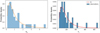 |
Fig. 1 Distribution of the low-frequency parameters used for the simulations with PSRPOPPY. Left: spectral index. Right: spectral turnover frequency. |
2 Estimation of the potential discoveries
2.1 Population synthesis
Realising a pulsar survey at low frequencies below 100 MHz allows us to probe a parameter space different from that of the majority of the other pulsar surveys carried out at higher frequencies. Also, an estimation of the potential pulsars to discover with the NPBS has been made using population synthesis.
The synthesis was performed using PSRPOPPY (Bates et al. 2014). According to the pulsar’s models, it generates a population of pulsars in the galaxy. Then, according to the given survey’s parameter, each pulsar’s flux is determined at the survey’s frequency. When the flux is greater than the sensitivity of the survey, the pulsar is marked as detected.
To generate the initial population, pulsars are created until a given number of discoveries by a reference survey is reached. Once the initial population is fixed, each pulsar is tested for a series of surveys, resulting in a number of detections and a number of discoveries for each survey.
For our modelling, we have chosen to generate our initial population using the most prolific survey, the PMPS (Manchester et al. 2001), considering the generated population as complete when the number of discoveries of the PMPS is reached. The periods of the population were modelled using the model of Lorimer et al. (2006) for a pulse width of 6%. The spatial distributions in Galactic radii and heights were defined from the model of Lorimer et al. (2006). The luminosity of the pulsars was determined following the model of Faucher-Giguère & Kaspi (2006). The interaction with the ISM is modelled using the model NE2001 (Cordes & Lazio 2003) to calculate the DM and using the model of Bhat et al. (2004) with the frequency dependence of −3.86 for the scatter broadening.
Discoveries previous to the NPBS have been modelled using the three parts of the HTRU survey (Keith et al. 2010), the Arecibo drift-scan survey (Deneva et al. 2013), the PALFA survey (Lazarus et al. 2015), the GHRSS survey, the GBNCC survey (McEwen et al. 2020), and the LOTAAS survey (Sanidas et al. 2019). LOTAAS is the most recent one and the closest to the NenuFAR frequencies, leading to a proper base for our simulation. However, contrary to the previous surveys, it was not included in PSRPOPPY, and we created a survey file for LOTAAS based to information provided by Sanidas et al. (2019).
The distributions and parameters listed above are the standard parameters of PSRPOPPY. However, this software was developed for modelling detections for higher frequency surveys than the NPBS. Consequently, it does not take the low-frequency spectral turnover into account, calculating the flux using a simple power-law. For this reason, we have adapted PSRPOPPY to the low frequencies by including the possibility of spectra with a double power-law. Thus, the generated pulsars follow either a simple power-law spectrum or a double power-law spectrum similarly described by the definition of Bilous et al. (2020) such as
 (2)
(2)
Here, S0 designates the reference flux at 1.4 GHz, νo the reference frequency (i.e. 1.4 GHz), and νt is the frequency of the spectral turnover. Two spectral indices are required: the high-frequency index αhi and the low-frequency index αlo.
For αhi, we used the distribution of Lorimer et al. (1995) which is the default model of PSRPOPPY. For αlo, a distribution has been fitted using the spectral indices below the turnover measured by Bilous et al. (2020). The distribution of the measured αlo is shown in the left panel of Fig. 1, and was fitted using a log-normal law such as
 (3)
(3)
The best fit was obtained for σ = 0.873 and µ = −0.208, corresponding to a mean low-frequency spectral index of 1.19 distributed with a standard deviation of 1.27.
In the same way, the distribution of the turnover frequency νt in the right panel of Fig. 1 was obtained from those measured by Bilous et al. (2020) and fitted with a log-normal law. The best fit was obtained for σ = 0.698 and µ = 5.030, corresponding to a mean frequency of 195 MHz distributed with a standard deviation of 155 MHz.
According to the results of Bilous et al. (2020), a spectral turnover does not seem to be present for all pulsars. An additional parameter was thus included, defining the fraction of pulsars with a turnover. For those with a turnover, αlo and νt were determined, and the flux was computed using the double powerlaw in Eq. (2). For generating our population, we have chosen a fraction of 50%.
The results of detection and discoveries are dependent on the initial population, leading to differences between simulations with various populations. Furthermore, PSRPOPPY also simulates the scintillation effect by increasing or decreasing the S/N of a pulsar. The scintillation has a random impact on the measured flux of a pulsar. Consequently, different runs of the same simulations (i.e. with the same simulated pulsar population) obtain different results for the number of detected pulsars.
Accordingly, multiple populations and simulations have been carried out to obtain average values of detections and discoveries. Thereby, 250 populations have been generated and for each of them, the simulation of the NPBS has been realised 250 times. The distributions of the number of detections and discoveries resulting from the 62 500 simulations are shown in Fig. 2. For both, an average number and an uncertainty representing one standard deviation were determined using a normal law fit. With this, based on PSRPOPPY, we can expect the NPBS to detect between 61 and 79 known pulsars and discover between 0 and 4 new pulsars. However, additional effects have to be taken into account before a final estimate can be obtained; these are discussed in the following section.
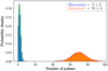 |
Fig. 2 Distribution of the numbers of discoveries and detections obtained by simulations with PSRPOPPY. The blue distribution on the left represents the number of discovered pulsars and the distribution in orange is the number of known pulsars detected for all the simulations. |
2.2 Widening of the emission cone
The results of PSRPOPPY are strongly dependent on the initial population, essentially generated according to the high- frequency discoveries (typically at 1.4 GHz). However, the discoveries of the recent surveys at lower frequencies show a larger fraction of slow pulsars than the ATNF pulsar catalogue. Surveys at lower frequencies are less sensitive in the directions of the Galactic plane because of a higher scattering compared to previous higher-frequency surveys. As mentioned by McEwen et al. (2020), the discovery distribution of low-frequency surveys is consequently shifted towards high Galactic latitudes, where pulsars are typically older and then slower. Furthermore, as mentioned by van der Wateren et al. (2023), the population accessible at a low frequency seems to be different from that observed at high frequency. A possible explanation for this is the widening of the emission cone at low frequencies (Tan et al. 2018). According to the RFM model, low frequencies are emitted at higher altitudes, where the emission cone is larger.
However, PSRPOPPY estimates the width of the emission cone using a relation without any frequency dependence (see Bates et al. 2014, for more details). As a consequence, one can expect a higher number of discoveries than predicted by PSRPOPPY.
The radius of the emission cone, ρ, can be described as a function of the period of the pulsar and the emission height (Lorimer & Kramer 2012). Fitting peaks separation, the emission height is modelled by Kijak & Gil (2003) as a function of the period P, period derivative Ṗ, and observing frequency ν. Combining the two equations, the radius ρ of the emission cone (in radians) can be described by the following relation:
 (4)
(4)
According to Emmering & Chevalier (1989), the related average fraction of sky covered by a pulsar’s beam, fcoν, is given by the equation:
 (5)
(5)
The orientation of the rotation axis of the pulsar relative to Earth is random. Then, the position of Earth is randomly localised in the sky sphere around the pulsar, following thereby a uniform distribution of the localisations on the sphere. Thus, this average sky coverage can be considered as the average probability that the emission at the observing frequency ν of a pulsar with a given period P and a given period derivative Ṗ crosses Earth.
For a given population of pulsars having similar characteristics, the initial population can be estimated by Ndet(ν0) / fcoν (ν0), where Ndet (ν0) is the number of pulsars detected at a reference frequency ν0. The average number of pulsars detected at another frequency ν can be then determined using the corresponding probability fcoν (ν).
However, especially at the NenuFAR frequencies, a strong constraint for the detection of pulsars is the pulse broadening caused by the scattering. According to Bhat et al. (2004), the scattering characteristic time τs can be related to the DM and the observing frequency. This scatter DM-dependent broadening leads to a maximum DM value, above which pulsars are unlikely to be detectable.
For the purpose of this model, the DM limit was defined as the DM corresponding to a scatter broadening (at the central frequency) equal to the pulsar period at 10% of the maximum amplitude. Because τs scales as ν−4, a pulse width equal to the period at the central frequency means that the pulsar is totally undetectable in a substantial fraction of the bandwidth (up to half of the bandwidth for a weak pulsar). Using the exponential equation of the pulse amplitude as a function of the scattering timescale, the scattering timescale can be related to the pulsar period. Then, based on the second-order polynomial in log(DM) of Bhat et al. (2004, Sect. 5.2), the based-10 logarithm of the DM limit log DMs can be calculated using the positive root (corresponding to a DM > 1 pc cm−3) such as
 (6)
(6)
Assuming the DM distribution of the detected pulsars is similar for all the observing frequencies1, the fraction of pulsars detectable at a given frequency can be estimated by the cumulative distribution fraction of the normalised DM distribution p(DM):
 (7)
(7)
For a given population of pulsars having the same characteristics, the final average number of discoveries Ndisc at the frequency ν (with ν < ν0) can be estimated as
 (8)
(8)
The last term in Eq. (8) represents the difference between detections (i.e. pulsars already known at higher frequencies), and new discoveries.
In the following, we classify the currently known pulsars into five populations, representing five regions of the P − Ṗ diagram: the millisecond pulsars (MSPs), the young pulsars such as the Crab pulsar, the normal pulsars, the high energy pulsars such as magnetars, and the slow pulsars. These populations were selected based on limits in the period, period derivative, and spin-down energy loss rate Ė. According to the detections of LOFAR (Sanidas et al. 2019; Bilous et al. 2020) and the NenuFAR pulsar census (Bondonneau et al., in prep.), only the normal pulsars and slow pulsars are expected to be detected by the NPBS.
For MSPs, selected such as pulsars with P < 60 ms and Ṗ < 10−16 s s−1, the combination of their short periods with the strong scatter broadening below 100 MHz results in a low probability to detect this type of pulsar with the NPBS. For a typical MSP, the DM limit DMs at 58 MHz is just 19.75 pc cm−3. Furthermore, the light cylinder of MSPs is considerably smaller than for other pulsars, resulting in an emission closer to the surface of the neutron star, even closer than prediced by the RFM (Kijak & Gil 1998). Therefore, although the RFM seems to hold for MSPs, the model for the emission altitude as a function of the period used here, and the subsequent widening of the cone, seems to be not valid for this type of pulsar.
For young pulsars, selected such as pulsars with P < 2 s, Ṗ > 10−16 s s−1, and Ė < 3 × 1026 J s−1, their surrounding generally generates a strong and variable scatter broadening. Although the DM limit for a typical young pulsar is 64.47 pc cm−3, such a DM represents only 6% of all the known young pulsars in the ATNF pulsar catalogue. Moreover, because of the particular surroundings of this type of pulsar, the average scattering characteristic time of this class of pulsar is likely longer than those provided by the relation of Bhat et al. (2004). Consequently, that leads to a low probability of detecting them with the NPBS.
Although they have long periods of several seconds, high- energy pulsars such as magnetars are difficult to detect in radio. Indeed, according to the McGill catalogue2 (Olausen & Kaspi 2014), there are merely six magnetars with persistent radio emission. Moreover, the majority is localised in the Galactic plane, resulting in large DM values and therefore strong scatter broadening. The calculation of the DMs at 58 MHz for this class provides a DM limit of 120.62 pc cm−3. However, in the set of high-energy pulsars, selected such as pulsars with P > 2 s and Ṗ > 5 × 10⁻¹³ s s−1, the one with the lowest DM in the ATNF catalogue has a DM of 178 pc cm−3 . Accordingly, we can presume this class of pulsars cannot be detected by the NPBS.
The first interesting class for the NPBS is that of normal pulsars defined such as pulsars with a period ranging from 60 ms to 2 s and Ė < 3 × 1026 J s−1. The second class is constituted by the slow pulsars defined such as pulsars with a period longer than 2 s and Ṗ < 5 × 10⁻¹³ s s−1.
For these two classes, the calculation of the radius of the emission cone and the subsequent values have been realised based on the median of the period 〈P〉 and the median of the period derivative 〈Ṗ〉 of the population (see Table 1). The scattering factor fsca has been calculated using a fit of the DM distribution of the respective population. Finally, uncertainties have been determined based on the median absolute deviations σ(P) and σ(Ṗ) of the period and period derivative distributions of each class. Thereby, the lower and upper edges of the associated uncertainty have been computed by comparing the minimum and maximum value of Ndisc for the four pairs (Pmin, Ṗmin), (Pmax, Ṗmin), (Pmin, Ṗmax), (Pmax, Ṗmax), where Pmin = 〈P〉 − σ(P), Pmax = 〈P〉 + σ(P), etc.
The vast majority of pulsar surveys were realised at frequencies higher than 300 MHz. For our purposes, the most relevant survey to compare with is LOTAAS. It is one of the most recent surveys, observing at frequencies lower than 300 MHz, and has detected and discovered a significant number of pulsars in the Northern Hemisphere. For this model, we have assumed that LOTAAS has detected all the pulsars that are above 100 MHz in the Northern Hemisphere. This is motivated by the high sensitivity of the LOFAR telescope and the relatively long integration time of the survey. With this, we have determined the potential average number of discoveries at a reference frequency of 135 MHz (the central frequency of the LOTAAS survey) and compared it to a frequency of 58 MHz (the central frequency of the NPBS).
For both classes of pulsars of interest, the DM limit DMs at 58 MHz is larger than the maximum DM of the NPBS (see Sect. 5.3). As a consequence, the scattering factors fsca at 58 MHz were calculated for the maximum DM of 70 pc cm−3 . At the reference frequency of 135 MHz, the LOTAAS survey searched for DM up to 546.3 pc cm−3, which is considerably larger than the two DM limits DMs . Hence, corresponding scattering factors at 135 MHz were determined using these two DM limits (164 and 215 pc cm−3).
The base pulsar population was provided by version 1.64 of the ATNF pulsar catalogue. The population parameters for each class were determined relative to the entire pulsar population satisfying the selection criteria. However, the majority of the pulsars are localised in the Southern Hemisphere. As a consequence, for each class, the base number of pulsars already detected Ndet (ν0) in Eq. (8) was determined by the number of pulsars satisfying the selection criteria and localised in the Northern Hemisphere (i.e. only those with a declination greater than 0°).
Applying Eq. (8), an average number between 21 and 23 normal pulsars and two slow pulsars could be potentially discovered at 58 MHz. These numbers have to be normalised by the observed sky area before a direct comparison with the result of PSRPOPPY; this is done in Sect. 2.4.
It should be noted that the numbers provided in this section do not take the difference in telescope sensitivity into account (in other words, all pulsars geometrically detectable are assumed to be detected). Also, the increasing flux of the pulsars and sky background towards low frequencies as well as the potential spectral turnover are equally not taken into account. As a consequence, these values rather represent a maximum potential number of discoveries in the case of similar flux and sensitivity. Still, it is clear that while the estimated number of pulsar discoveries at a low frequency suffers from spectral turnover and a high sky background, some additional discoveries can be expected due to the widening of the emission cone.
Modelling parameters of the emission cone widening and expected number of discoveries.
2.3 Steep-spectrum pulsars
Without any widening of the emission cone of the pulsars, low- frequency discoveries could be realised thanks to the increase of their flux density towards low frequencies. In this case, certain pulsars could have a sufficient flux to be detected only by low- frequency surveys (even with a lower-sensitivity telescope). For a discovery below 100 MHz, this behaviour is expected for pulsars presenting a steep spectrum with a spectral index greater than most of the currently known pulsar population (and no low-frequency turnover).
Simulations with PSRPOPPY are based on a population created to provide a realistic but limited number of pulsars detectable from Earth. At the opposite, Monte-Carlo simulations can be carried out to generate a large number of mock pulsars, allowing us to determine the most likely spectral indices of potential discoveries. For this work, spectral characteristics have been defined for 109 modelled pulsars. We performed calculations to identify the population of mock pulsars that are detectable by the NPBS on the one hand, but not detectable by the LOTAAS survey on the other hand. Simulations consisted of computing the flux of a modelled pulsar at 58 MHz (the central frequency of the NPBS, see Sect. 3.3) based on its flux density at 135 MHz (the central frequency of LOTAAS) following Eq. (2).
Using a reference frequency of 135 MHz for the reference flux has an advantage compared to the population synthesis carried out by PSRPOPPY, which is based on a luminosity distribution defined at 1.4 GHz (Faucher-Giguère & Kaspi 2006). Using the minimum sensitivity of LOTAAS and the NPBS, the limit spectral index (for a simple power-law spectrum) required for detection by the NPBS without being detected by LOTAAS can be estimated by
 (9)
(9)
Using F(ν) = 1.2 mJy as the minimum flux density of LOTAAS (Sanidas et al. 2019) at a central frequency νref = 135 MHz, and F = 10 mJy as the minimum sensitivity of the NPBS (see Sect. 7.2) at the central frequency of 58 MHz (see Sect. 3.3), the absolute value of the spectral index has to be greater than 2.51 for a pulsar to be solely discovered by the NPBS. Such a pulsar would have a flux density of just 3 µJy at 1.4 GHz. Such a flux is close to the minimum sensitivity of 1 µJy for the GPPS survey performed with the telescope FAST (Han et al. 2021). However, the luminosity distribution underlying PSRPOPPY is constrained in order to reproduce the measured flux density distribution at 1.4 GHz. As a consequence, it is unlikely to generate pulsars with a flux lower than 3 µJy. The use of a luminosity distribution at 1.4 GHz could thus introduce a bias relative to the possibility of discovery for a survey at a very low frequency. Accordingly, the simulations presented in the following are performed based on a flux density at 135 MHz rather than 1.4 GHz. This allows us to take into account pulsars not detectable at 1.4 GHz and thus only visible at low frequencies.
At NenuFAR frequencies, the sky temperature is the dominant contribution to the system temperature. Also, with a difference of a factor of about 50 between ‘hot’ and ‘cold’ regions, the position of a pulsar relative to the Galactic plane significantly modifies the sensitivity of the NPBS (see Sect. 7.2). Hence, the value of the lowest spectral index is dependent on the position. Figure 3 shows the sky map of the lowest spectral index necessary to solely detect a pulsar with the NPBS. The mean typical pulsar spectrum has a mean negative slope of absolute value 1.6 (Jankowski et al. 2018). Close to the Galactic plane, the required spectral index reaches very high absolute values, leading to a very low probability of discovering a pulsar at these locations. In the coldest parts of the sky, in particular on the left of Fig. 3, the spectral index needs to have an absolute value of at least about 2.5. Such pulsars exist, but are rare (e.g. they represent only ~2% of the population studies by Jankowski et al. 2018). Accordingly, potential discoveries should present spectra significantly steeper than those of the current pulsar population.
In the simple case of pulsars with spectra described by a simple power-law F = F135 ⋅ (ν/135 MHz)−α, the flux density can be determined based on four parameters: a single spectral index α (identical for all frequencies), a flux density at 135 MHz F135 , and the coordinates in the Galactic frame ɡl and ɡb. The spectral index was defined according to the distribution of the absolute values of spectral indices from Bilous et al. (2016) with a log-normal distribution of mean 1.42 and standard deviation 0.41. For a pulsar not detected by LOTAAS, its flux density at 135 MHz can be located between 0 and the minimum sensitivity of LOTAAS of 1.2 mJy. Because such pulsars are unknown, we do not know the distribution of their flux at 135 MHz. The flux at 135 MHz was thus defined using a uniform distribution between 0 and 1.2 mJy. Because of the strong dependency of the sensitivity of the NPBS, a sky position has to be set for each model. A Galactic longitude and latitude were defined using the model of Lorimer et al. (2006) for the radial and height distributions. Based on this position, the sky temperature was calculated using the sky map of Haslam et al. (1982) and the sensitivity at 58 MHz was determined with the radiometer equation (Dewey et al. 1985).
Figure 4 presents the posterior distributions of the four parameters, corresponding to the models with flux at 58 MHz greater than the sensitivity of the NPBS at the coordinates (ɡl, ɡb). As expected, the larger the flux at 135 MHz, the higher the probability of detecting the pulsar with the NPBS. The prior distribution of spectral indices has a mean of 1.6 with a most likely value approximately of 1.8 (in absolute value, see Fig. 6 of Jankowski et al. 2018). However, the posterior distribution can be fitted with a log-normal distribution of mean 3.40 with a standard deviation of 0.53 and a most likely value of 3.18. Hence, the likely pulsars detectable by the NPBS have a spectral index significantly larger, corresponding to the tail of the prior lognormal distribution. A pulsar with a spectral index of 3.40 and a flux density of 1.2 mJy at 135 MHz (i.e. undetected by LOTAAS) would have a flux density at 1.4 GHz of about 0.42 µJy. Such a flux density is indeed smaller than the minimum sensitivity of about 1 µJy for the GPPS survey of FAST (Han et al. 2021). Pulsars with such steep-spectra emitting at low-frequency could be thus solely detectable below 100 MHz.
Concerning the spatial distribution, the likely detectable pulsars are localised close to the Galactic Centre, but excluding this region itself. Because the temperature of the Galactic centre is greater than 104 K, it is indeed unexpected to detect pulsars in this area except for very bright pulsars. The most substantial probability localised around the centre rather than totally outside seems to be consistent with the fact that pulsars are essentially localised within the galaxy.
The present simulation does not take the diverse effects produced by the ISM into account. The closer the pulsar is to the Galactic centre, the more significant is the DM and the scatter broadening. Therefore, including the ISM effects, the spatial distribution should be more spread.
In the case of pulsars with spectra following a broken powerlaw  , the simulation is more complex. Because the spectrum is not monotonic, even very steep-spectrum pulsars can be undetectable at the NenuFAR frequencies. It is, therefore, necessary to add two parameters to the previous model: a second spectral index αl describing the low-frequency part of the spectrum and the frequency of the spectral turnover νt . The four other parameters were generated similarly to the case of the simple power-law, where the previous spectral index α corresponds to the high-frequency spectral index αh for the broken power-law case. The two added parameters were defined using the fitting relations determined for the PSRPOPPY simulations (see Fig. 1 and Sect. 2.1), which were based on the data of Bilous et al. (2020).
Figure 5 shows the posterior distributions for the six parameters of the simulations with a spectral turnover. For the flux density at 135 MHz and the spatial distribution, the distributions are similar to the simple power-law case. Also, as for the simple power-law case, the distribution of the high-frequency spectral indices corresponds to the tail of the prior distribution. Nevertheless, as expected, the distribution is shifted towards slightly larger values, following a log-normal distribution of a mean of 3.66 and a standard deviation of 0.60. For the low-frequency spectral index, the posterior distribution follows a log-normal distribution of a mean of 1.29 and a standard deviation of 1.23. The posterior distribution is very close to the prior distribution of a mean of 1.19 and a standard deviation of 1.27.
Finally, different pulsars have different turnover frequencies. Figure 1 shows that the most likely value for the turnover frequency is close to 100 MHz, and its average is around 200 MHz. Pulsars with a lower turnover are more likely to be discovered by the NPBS. For a turnover frequency below 58 MHz, we are in the limit case of the simple power-law spectrum, requiring smaller spectral indices to be detected by the NPBS. In the case of pulsars with spectra following a broken power-law, the most likely pulsars expected to be discovered by the NPBS have a spectral index of 3.4 at high frequency, a spectral index of 0.5 at a low frequency, and a turnover frequency close to or below 58 MHz.
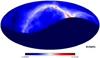 |
Fig. 3 Sky map in ecliptic coordinates of the lowest spectral index required to discover a pulsar with the NPBS compared to the reference survey of LOTAAS. |
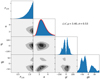 |
Fig. 4 Posterior distributions for simulations using a simple power-law. Parameters are: the spectral index α, the flux at 135 MHz Flot (the central frequency of LOTAAS), and ɡl and ɡb correspond to the Galactic longitude and latitude. |
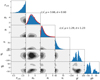 |
Fig. 5 Posterior distributions for simulations using a broken power-law. Parameters are: the high-frequency spectral index αh , the low-frequency spectral index αl, the spectral turnover frequency νt, the flux at 135 MHz Flot (the central frequency of LOTAAS), and ɡl and ɡb correspond to the Galactic longitude and latitude. |
2.4 Estimate of NPBS discoveries
Using the three simulations (Sects. 2.1–2.3), a rough estimation of the number of potential discoveries by the NPBS may be realised. According to the population synthesis including the low-frequency spectral turnover, two new pulsars are expected to be discovered. The population synthesis is based on the currently known pulsar population, without potential steep-spectrum pulsars which would mostly be detectable at low frequencies; it also does not take into account the (statistical) widening of the emission cone at low frequencies. Hence, this expectation of two pulsars should be considered as a lower limit.
On the opposite side, the expectation of 23 new pulsars obtained by the widening of the emission cone (assuming RFM) does not take into account the survey sensitivity, the observed fraction of the sky, or detailed characteristics of the survey (from observing setup, search methods,…). It can be thereby considered rather as a maximum number of discoveries. To compare to the lower limit, we have taken the observed sky fraction into account. At NenuFAR frequencies, we are mostly sensitive to nearby pulsars, and can thus roughly assume a homogeneous sky distribution of the pulsars. The NPBS covers the sky >+39° of declination, that is, 37% of the northern sky. We can thus expect the NPBS to discover 8 normal pulsars and one slow one. A future extension of the NPBS to 0° of declination would increase these numbers to 21 normal pulsars and two slow ones.
Finally, Sect. 2.3 provides us constraints on the potential discovered pulsar parameters, especially on the high-frequency spectral index and flux at 135 MHz. The population synthesis generates its pulsar population following the current spectral index and flux distributions. However, the posterior distribution of the high-frequency spectral index in Figs. 4 and 5 corresponds to the tail of the entire prior distribution. Consequently, merely a small number of steep-spectrum pulsars can be generated. Also, logically, the current flux prior distribution does not permit for the generation of a large number of pulsars with a low flux at frequencies between 100 and 150 MHz, which is the requirement to get pulsars not detected above 100 MHz and detectable with NenuFAR.
The consequence is that if there are no more pulsars with steep-spectrum mainly emitting at low frequencies than expected by the current distributions, the number of two discoveries provided by the population synthesis is a good estimation. Conversely, if there exists a larger number of such pulsars, the estimation of two discoveries might be increased by a factor impossible to evaluate now. In the same way, the estimation obtained using the widening of the emission cone is based on the current number of pulsars (in the ATNF catalogue), which do not contain such a pulsar population. Hence, if it exists, this estimation might be equally increased.
To support the hypothesis of such a population, van der Wateren et al. (2023) indicate LOTAAS discoveries presented on average spectra steeper than those of the population studied by Jankowski et al. (2018), which is used in the simulations above. One can deduce that if low-frequency surveys find a very small number of new pulsars, strong constraints could be evaluated on: the existence of a population of steep-spectrum pulsars emitting at low frequencies; the widening of the emission cone because of the RFM.
3 Observations
3.1 The radio telescope NenuFAR
NenuFAR3 is a new phased array telescope located at the Nançay Radio Observatory (ORN). It currently comprises 80 mini-arrays of 19 antennas each, spread over a disk-shaped area with a diameter of about 400 meters. For beam-formed observations, the telescope will reach its nominal effective area (96 mini-arrays of 19 antennas, that is, a total of 1824 antennas) during 2024.
NenuFAR can observe the sky from 10 MHz (just above the ionospheric cutoff) to 85 MHz (corresponding to the lower edge of the FM band). To observe, an analogue beam is formed, corresponding to the sum of the signals of all the antennas of an MA. The signals of the different MAs are then digitally summed to form digital beams contained within the analogue beam, and with a considerably smaller size. All beam-formed observations of NenuFAR currently use the backend UnDySPuTeD (Bondonneau et al. 2021), which allows to arrange a total processed bandwidth of 150 MHz into four digital beams of 37.5 MHz each. These four beams can be steered independently, provided they remain within the analogue beam of about 8° of FWHM at 85 MHz defined by the mini-arrays (see Bondonneau et al. 2021, for details). More details on NenuFAR can be found in Zarka et al. (2020) and the forthcoming NenuFAR instrument paper (Zarka et al., in prep.).
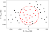 |
Fig. 6 Map of NenuFAR showing the 56 mini-arrays available in 2020. Dashed red line: circle of 210 m diameter defining the sub-array used for the NPBS. Red points: the 25 mini-arrays used for the NPBS. Black points: mini-arrays not used for the NPBS. Two mini-arrays within the red circle were excluded due to high RFI levels. |
3.2 Selection of the sub-array
In 2020, at the time of the definition of the NPBS, NenuFAR still was in its ‘Early Science Phase’. At that time, NenuFAR was constituted of 56 mini-arrays located in an ellipse of about 200 × 400 meters (see Fig. 6). The beam shape is a function of the projected area of the telescope in the sky. The ellipticity of the whole NenuFAR array would therefore result in an elliptic beam. Moreover, neither the major nor the minor axis of the NenuFAR area was aligned with the east-west axis. Consequently, the elliptic beam has an angle relative to the azimuth and elevation axes dependent on the azimuth and elevation of the source. With such a beam, it is very difficult to do a regular and optimised tiling of the sky. We have removed the dependence relative to the azimuth by defining a circular beam at the zenith. Although the size is still dependent on the elevation, the shape is always aligned, allowing for an optimized tiling.
In order to ensure a circular beam at the zenith, the telescope must have a circular shape on the ground, requiring the selection of a circular sub-array having the greatest possible effective area or gain. To determine the optimal configuration, the beam at the zenith was modelled for 7930 different configurations using the python programme NENUPY4 (Loh & Girard 2020), which is a dedicated tool developed to model the NenuFAR beam. Configurations correspond to subarrays of MAs contained inside circles with different centroids localized on the NenuFAR area. For each centroid location, four diameters were tested: 200, 205, 210, and 220 m. For each configuration, the beam radius at the zenith was determined for every azimuth. Here, we define the beam radius as the radial distance where the gain is attenuated by −3 dB relative to the gain at the centre (i.e. the FWHM of the beam). The ellipticity of the beam was then calculated using the standard deviation of the radius at −3 dB around the zenith (with a value of 0 representing a circular beam). Finally, the global average gain of the beam was computed. Because of we do not know the location of a pulsar within the beam, the global gain was determined as the average gain of the beam inside the limit of −3 dB.
For each of the four diameters, the map of ellipticity was compared with the map of gain to identify the optimal centroids (i.e. we searched for a configuration having a circular shape and a high average gain). As shown in the map of NenuFAR (as it was in 2020) in Fig. 6, the final configuration is a selection of 25 mini-arrays (red points) distributed on a disk (the dashed red line) of 210 meters in diameter located at 0 m in the north-south axis relative and at +5 m in the east-west axis relative to the centroid of NenuFAR (computed with the then available 56 miniarrays). We can notice two subarrays located in the south of the circle which were not retained. These were removed from the list of MAs due to radio frequency interferences (RFIs) generated by two air-conditioning units situated near the southernmost MA.
3.3 Selection of the central frequency
NenuFAR can observe from 10 to 85 MHz, with a relatively flat bandpass between 25 and 75 MHz, resulting in a constant telescope sensitivity in this range (Zarka et al., in prep.). Consequently, observing one target with a bandwidth of 75 MHz is less efficient than observing two targets with a bandwidth of 37.5 MHz at the frequency where NenuFAR is most sensitive. For the NPBS, the bandwidth has therefore been fixed to 37.5 MHz, and a search for the best central frequency was performed.
One of the challenges of the NPBS is its large fractional bandwidth. The diameter of the beam, defined as the FWHM, is considerably smaller at the highest frequency than at the lowest frequency of the survey (approximately a factor of three between 25 and 75 MHz). As a result, the sky coverage is inhomogeneous, with the emergence of overlapping pointings at the lowest frequencies or/and of gaps between pointings at the highest frequencies. In order to obtain an optimised sky coverage for the entire bandwidth, the observing band has to be carefully chosen.
We have simulated different pointing grids as a function of two parameters. The first one is the central frequency. Given that the bandwidth must be placed in the range of 25–80 MHz, twelve central frequencies linearly spaced between 40 and 62 MHz have been tested (finer steps have been used in a second iteration). The second parameter is the overlap rate corresponding to the fraction of the radius of the beam that overlaps with the adjacent beam at the central frequency (see Sect. 3.5). For each central frequency, overlap rates between 0 and 1 have been tested, with a step size of 0.05 (finer steps have been used in a second iteration).
We have simulated one pointing grid for each combination of these two parameters. Two criteria were used: the first criterion was to have a fraction less than 2.5% of unobserved survey sky (i.e. outside the FWHM of all beams) over 80% of the bandwidth; the second criterion was to have a fraction of unobserved sky of less than 12.5% at the highest frequency of the NPBS.
For each simulated grid, the fraction of sky coverage was measured for 21 frequencies linearly spaced in the bandwidth. Based on the results, we have chosen a central frequency of 58.0 MHz with an overlap rate of 0.63 to define the pointing grid of the NPBS. This central frequency is close to the maximum allowed by the bandwidth, and thus also reduces the problems of dispersive smearing and scattering to its minimum.
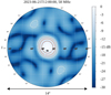 |
Fig. 7 Digital beam of NenuFAR in the configuration of the NPBS modelled at the zenith for a frequency of 58 MHz. Contours represent the gain attenuation of −3 (corresponding to the FWHM of the digital beam), −6, −9, and −12 dB, respectively. White contours defining the two sidelobes around the main lobe (as well as the outer contours of the main lobe) correspond to the gain attenuation of −12 dB. |
3.4 The pointing grid
The sensitivity of NenuFAR is proportional to its projected area as seen from the observed source, and consequently to the source elevation. In order to maximise the sensitivity, we required that each pointing is observed during its meridian transit, corresponding to the moment of maximum elevation.
At the meridian transit, there is a direct relation between the declination and the elevation of the pointing. The tiling of the sky along the declination axis can be thereby done successively, that is, starting from 90°, and adding beams at lower declination ring by ring, taking into account the elevation-dependent beam size. For each declination value on the pointing grid, pointings are then uniformly distributed along the right ascension axis.
This first run of the NPBS was planned with the aim to observe as much of the northern sky, starting from the north celestial pole and going as low as possible in declination with a total of 960 hours of available observing time. With this, the final pointing grid is composed of 7692 pointings divided into 51 ‘rings’ of pointings at a fixed value of declination. This allows covering the northern sky from the north celestial pole down to a minimum declination of 38.7°.
At the central frequency of 58 MHz, the NPBS pointings have a constant diameter of 1.44° in azimuth, an average diameter of 1.49° in elevation, and an average beam surface of 1.69 deg2. In elevation, the beam diameter varies from 1.44° for a declination of 42.8° (the zenith for NenuFAR) to 2.07° at 38.7°. These variations correspond to a surface between 1.62 deg2 for the smallest beam and 2.50 deg2 for the largest one. A model of the digital beam used for the NPBS computed at the central frequency around the zenith is shown in Fig. 7.
With respect to frequency, the angular beam diameter at the zenith varies from 2.10° at 39 MHz to 1.04° at 76 MHz, corresponding to a beam surface of 3.40 deg2 at 39 MHz and 1.05 deg2 at 76 MHz. The pointings have an average angular separation of 0.98°, resulting in an average sky coverage of 98.4% at 58 MHz, and 90.2% at the maximum frequency of 76 MHz. The general characteristics of the observational setup and pointing grid used for the NPBS are summarised in Table 2.
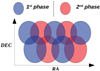 |
Fig. 8 Scheme presenting the principle of the two phases of the NPBS. Blue ellipses: pointings observed during the first phase of the NPBS. Red ellipses: pointing observed during the second phase of the NPBS. |
General characteristics of the NPBS pointing grid.
3.5 Scheduling of observations
To define the required observing time per pointing, we start from the time used by the NenuFAR pulsar census, which led to the first NenuFAR pulsar catalogue (Bondonneau et al., in prep.). For this census, all known pulsars in the sky observable by NenuFAR have been observed (over 600 pulsars with DM ≤ 100 pc cm−3), with an elevation-dependent observing time. In this census, the minimum observing time was set to 25 minutes. 184 non-recycled pulsars have been detected in the range of 10–85 MHz, 100 of which had never been seen before in this frequency range. This census serves as the reference point for all NenuFAR pulsar observations, including the present blind survey which aims to the detection of new, undiscovered pulsars. Hence, for the NPBS, we have required a minimum duration of 25 minutes.
Up to four digital beams (or pointings) of 37.5 MHz can be computed in real-time by the backends (see Sect. 3.1). Also, these four digital beams must be contained inside the analogue beam of NenuFAR whose minimum FWHM at 85 MHz is 8°. Hence, to avoid a significant loss in sensitivity, it is required that the digital beams are located around the centre of the analogue beam and spaced by less than 5° to avoid placing a digital pointing on the edge of it. For each observation of the NPBS, a group of (up to) four contiguous pointings is selected, all having their meridian transit at the middle of the observation, plus or minus 8 minutes. The analogue beam is set at the average sky position of the corresponding pointings. With four pointings per observation and a limited total available time for this first run of 960 hours, the maximum duration of the observations is of 30 minutes. Finally, because there are a few minutes of overhead required to re-point the beams of NenuFAR, the duration was set to 27 minutes.
In order to maximise the sensitivity to weak signals and increase the likelihood of detection, the time slots for observations have been chosen in a way to minimise the influence of RFIs. Following the analysis of the RFI situation for NenuFAR (Bondonneau et al. 2021), we have restricted NPBS observations to only take place during nighttime, more precisely between 21 h and 6 h UTC.
Because the grid has been defined using an overlap between neighbour pointings, we have chosen to divide the observing programme into two phases. As shown in Fig. 8, the first phase consists of observing every second pointing, allowing for observing more than half the targeted sky in less than half the total time. The second phase consists of filling in the sky coverage by observing the remaining pointings.
The observations of phase one have started in August 2020. The left panel of Fig. 9 presents the evolution of the observation of phase one, month by month, up to 31st July 2021 (corresponding to the end of the main observing programme for phase one). Observations of phase one are almost complete since May 2022 with merely a group of eight pointings which have to be repeated due to excessive RFI at the time of the observation (Summer 2022 and Summer 2023) due to thunderstorms.
The observations of phase two started in July 2021 and, as presented in the right panel of Fig. 9, the main observing programme is finished since August 2022 with about 97% of the pointings observed. The observation of the remaining pointings is still ongoing. As of the 1st of September 2023, 20 pointings need to be observed.
In total, 7 664 pointings have already been observed, representing 99.6% of the grid of the NPBS (Fig. 9). The remaining pointings of phases one and two will be observed during the first semester of 2024.
4 Pre-processing
4.1 Frequency and time resolution
In a survey, the DM of not-yet-discovered pulsars is not known a priori. In order to apply coherent dedispersion (Hankins & Rickett 1975) in order to correct for the intra-channel smearing (see Sect. 1), one would have to do so either during the observation (which is computationally not feasible), or one would have to store the raw voltage data (which would lead to data unreasonable data volumes). To be able to manage the data volumes of the NPBS, the observations are pre-reduced before the final analysis, and we have to resort to incoherent dedispersion. However, at NenuFAR frequencies, the dispersion is substantial and rapidly increases towards low frequencies, resulting in a dispersive delay seven times longer at the lowest frequency of 39 MHz compared to the highest one of 76 MHz. Therefore, the dispersive smearing of a pulse within a frequency channel is not negligible. For a given DM, observing frequency ν and channel bandwidth Δv, it can be expressed as follows:
 (10)
(10)
Figure 10 shows the intra-channel dispersion smearing as a function of the channel bandwidth between 0.5 kHz and the standard frequency resolution of NenuFAR of 195.3125 kHz. The smearing is computed at the lowest frequency of the NPBS of 39 MHz for five values of DM: 1, 20 (according to the ATNF catalogue5 Manchester et al. 2005, there are 197 known pulsars with a DM below this value), 50 (759 known pulsars), 70 (1037 known pulsars), and 100 pc cm−3 (1342 known pulsars). For a standard pulsar observation of NenuFAR, that is, using a frequency resolution of 195.3125 kHz (Bondonneau et al. 2021), this results in an intra-channel dispersion smearing of about 27 ms in the lowest channel already for a DM of 1 pc cm−3 , and the smearing exceeds one second for a DM of 50 pc cm−3 . Consequently, it is necessary to use a finer frequency resolution for the NPBS.
To do this, the pointings of the NPBS have been observed using a specific observation mode called ‘dynamic spectrum’. In this observing mode, the backend still receives the standard data stream sent by the beamformer, that is, a frequency band of 37.5 MHz divided into 192 channels with a frequency resolution of 195.3125 kHz and a time resolution of 5.12 µs. In each frequency subband, channelisation is then performed by the backend using an FFT on these data. For the NPBS, we have chosen to increase the frequency resolution by a factor of 128 in order to finally divide the band of 37.5 MHz into 24 576 channels with a channel bandwidth of 1.529 kHz each. With this, intra-channel dispersion is reduced but still not completely negligible (see dashed black lines in Fig. 10), with a smearing of approximately 20 ms for a DM of 100 pc cm−3.
As smearing does not allow us to resolve fine structures, there is no need to keep an exceedingly high time resolution in our data. We have, therefore, chosen to down-sample the data by a factor of 16 (in addition to the FFT length of 128) using an averaging by blocks of 16 initial time samples to get a time resolution of 10.486 ms. In view of the 7692 pointings required for the NPBS, this reduction in time resolution allows for saving a significant amount of disk space.
As a result, for high DM pulsars (DM > 50 pc cm−3), observable profile features are limited by the intra-channel DM smearing. For observations of lower DM pulsars (DM < 50 pc cm−3), the intra-channel broadening is smaller than the sampling time, and the smallest profile features are limited by the time resolution of the survey.
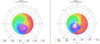 |
Fig. 9 Stereographic projection of the observed sky month by month. Left: observations of phase one from August 2020 in red to July 2021 in purple. Right: observations of phase two from July 2021 in red to August 2022 in purple. Grey areas represent sky areas that remain to be observed. |
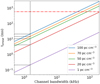 |
Fig. 10 Intra-channel dispersion smearing at 39 MHz as a function of frequency resolution (ranging from 0.5 to 195 kHz). The five coloured lines correspond to five different DM values: (from the bottom to the top) 1, 20, 50, 70, and 100 pc cm−3 . The red dashed-dotted line corresponds to the median of the periods of all the non-MSP pulsars according to the ATNF catalogue (Manchester et al. 2005). The black dotted line corresponds to the frequency resolution of 1.529 kHz used for the NPBS and the associated smearing for the five DM values. |
4.2 Data characteristics and formats
The data are first recorded in a type of file specific to this observing mode called ‘dynamic spectra’, with the full polarisation information in floating point values of 32 bits. Compared to a raw ‘waveform’ observation of NenuFAR, this increases the number of frequency channels by a factor of 128. At the same time, the time resolution is decreased by a factor of 2048. Together, this allows us to reduce the size of each file by a factor of 16. As a result, for each pointing, we obtain a file of 56 GB, corresponding to a total disk space of about 430 TB.
However, the size of these spectra files is still too large, and the full polarisation information is not necessary in the context of a survey. Hence, the spectra files are treated as intermediate files. The 32-bit floating full Stokes data are converted to total intensity 8-bit integer. In every channel, estimations of the median value and the rms are performed over 1.7s (7s after April 2022) using 3 successive steps, removing samples outside the ±3 rms range for the latter two. Boundaries for the 8-bit integer conversion are then chosen to be ±3 rms around the median. As a result of this conversion, the data size is reduced by another factor of 16, leading to a file size of 3.5 GB. For the whole survey, this amounts to 27 TB of observed data.
These reduced datasets are written out in standard FILTERBANK format, which can be used as input for the PRESTO software. PRESTO (Ransom 2001)6 was specifically developed for efficient pulsar and transient searches and has already obtained a substantial number of discoveries of pulsars in several previous surveys. The search pipeline used for the NPBS is also based on the software PRESTO, as will be described in Sect. 5.
5 Data processing
5.1 Flattening
To point a sky direction, every mini-array of NenuFAR generates an analogue beam using physical delay lines. Thus, the pointing follows a pre-defined grid (see Zarka et al. 2020 for more details) and has to be repointed every six minutes to follow a source. In a second step, the phasing of the MAs is realised by a digital phasing to generate the digital beam (see Sect. 3.5). This phasing is updated every 10 seconds to follow the source. These two stages of tracking adjustments create discontinuities in the time series appearing as periodic jumps in the baseline. Figure 11 shows a part of the frequency-integrated time series of an observation of the NPBS. The plot is zoomed around a tracking adjustment of the analogue beam. The tracking adjustment of the analogue pointing appears as a sudden decrease, followed by a logarithmic recovery caused by the electronic start of the relays in every sub-array. Within this logarithmic shape, one can identify smaller discontinuities every 1.7 seconds created during the generation of the ‘spectra’ files (see Sect. 4.2).
These baseline variations lead to an increase in the standard deviation and a modification of the median value of the time series. However, the RFI mitigation performed in the next step (see Sect. 5.2) is based on diverse statistical comparisons of chunks of time or frequency. As a consequence, the presence of these jumps decreases the efficiency of the RFI mitigation, and some small-amplitude RFIs will remain undetected. Additionally, for weak pulsars, overly large changes in the statistics could result in normalised amplitude lower than the detection thresholds. In order to correct (or at least to partly absorb) for these different jumps in amplitude before RFI removal and pulsar detection, a first step of flattening of the data must be realised in time and frequency.
The aim is to improve the data statistics and the major RFIs are then searched in time and frequency. In order to be sure to have a bandpass totally flat, the process starts with its normalisation (i.e. flattening along the frequency axis). For each frequency channel, the entire time series of the observation is normalised, allowing to already set to the median all the channels entirely saturated by an RFI. Firstly, in the normalised bandpass, all time samples in a channel with a deviation greater than 3σ are set to the median of the bandpass. Secondly, in the entire time series integrated in frequency, all channels of a time sample which deviate more than 3σ from the median of the time series are set to the median of the time series.
For the flattening of the time series, the positions of the jumps caused by the tracking adjustments of the analogue beam are searched in the frequency-integrated time series. Then, for each channel, in each block of six minutes, a running average is computed by a convolution with a Gaussian window. Compared to a simple running average by block, the convolution with a Gaussian has the advantage of reducing the edge effects by maximising the weights of data around the central point. The initial (non-convolved) time series of the channel is then flattened by subtracting this running average.
During the generation of the spectra file (see Sect. 4.2), scales and offsets are computed for time blocks of 1.7 s (7s for observations after April 2022) for every channel. This normalisation by block results in a residual slope due to the initial slope of the logarithmic shape of the baseline. As a consequence, the Gaussian used for the smoothing of the discontinuities must be considerably smaller than these blocks of 1.7 s to avoid corrupting the average. On the opposite side, it has not to be overly small to avoid erasing pulses. After some tests for different widths for the Gaussian window curve, we have chosen a window with an FWHM of 356 ms (corresponding to 34 time samples). This window size allows us to reduce the corruption of the average by the baseline changes introduced by the pointing of the telescope.
According to the ATNF catalogue, there are merely four pulsars with a pulse width at 50% of peak greater than the FWHM of this Gaussian. Nonetheless, to avoid potentially smoothing extremely wide pulses, the size of the window was set to five times the FWHM of the Gaussian window function, corresponding to 1.845 s. With this, the Gaussian window should be sufficiently large so that the average is not solely computed on the on-pulse of a pulsar.
The efficiency of the flattening scheme was validated by test observations. In June 2020, preliminary test observations were made by observing 24 pulsars using the observational setup of the NPBS, and the search pipeline was applied. From this set of pulsars, J1627+1419 was the faintest detection. Using the original data (i.e. without any flattening), it was detected in the dispersed time series (see Sect. 5.3) only for two DMs with a final significance calculated by ACCELSIFT.PY (see Sect. 5.5) of 9.10σ. Using the flattening step, it was found in 22 DM values around its DM of 32.17 pc cm−3 with a final significance of 9.20σ. While the significance results are close, the number of DM values is equally an important criterion in the detection pipeline. The sifting step requires a signal for at least two consecutive DM values (see Sect. 5.5). Without flattening, the detection only for two DMs close to the correct DM means that a slightly weaker pulsar would have remained undetected. With flattening, the detection of the signal of J1627+1419 for DMs at ±0.1 pc cm−3 around the true value means that a weaker pulsar should continue to appear in several DMs, and thus remain detectable.
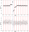 |
Fig. 11 Comparison of the frequency-integrated time series of an observation of the NPBS before and after the flattening step. Top panel: part of the original time series with the tracking adjustment of the analogue beam of NenuFAR just before 720 s (blue dotted line). Bottom panel: same part of the time series after the flattening step. Red dashed lines indicate the positions of the short discontinuities every 1.7 s generated during the data conversion into an 8-bit filterbank. |
5.2 RFI mitigation
During the flattening step, only the strongest RFIs were removed. Now that the data are flattened, we need to perform a more precise RFI search. This step uses the programme RFIFIND of PRESTO, which is based on the statistical comparison between different subsets of data: global data, frequency channel, time integration (all channels in a specific time sample) and time blocks corresponding to a time sub-integration within a channel. For each of these, the median, the standard deviation, and the maximum of the Fourier power are computed and compared to determine bad parts of the data.
The flagging of data considered as RFIs is carried out by flagging the time blocks. For the NPBS, the duration of time blocks was set to 671 ms. Such a duration is longer than the width of almost all the pulsars (according to the ATNF catalogue, only five pulsars have a width at 10% of the maximum amplitude >600 ms), such that the ON-pulse region does not strongly modify the statistics within the block. As is usual for RFIFIND, a time block is rejected if its maximum Fourier power is larger than the summed FFT power level corresponding to a Gaussian significance of 3σ. A time block is equally flagged if its median or standard deviation deviates more than 3σ from the median or standard deviation of the channel, integration, or global data. Furthermore, channels with more than 30% of bad sub-integrations, as well as sub-integrations with more than 30% of bad channels, are rejected.
We also remove ‘birdies’, corresponding to periodic signals appearing in the time series, but which are not of astrophysical origin. As is typical for RFI, birdies are not dispersed (i.e. they have a DM of 0 pc cm−3). The identification of birdies is realised by computing the FFT on the frequency-integrated time series of the full observation. The FFT is realised with the programme REALFFT of PRESTO. All Fourier frequencies with an amplitude above 5σ are considered as birdies and are listed in a file. This file will be used to ignore the Fourier frequencies of these birdies during the search for periodicities (see Sect. 5.4).
For every observation, typically about 12% of data are flagged, particularly above 70 MHz due to military and police gendarmerie transmissions.
5.3 Dedispersion
The search for pulsars used for the NPBS is based on the search for periodic signals in the time series integrated in frequency. Consequently, it is required to search for the DM in order to increase the S/N of a potential pulsar signal. Because the DM of a potential pulsar is unknown, we need to dedisperse data for different trial DM values.
The dedispersion step is the longest of the processing pipeline. As a consequence, this step has to be optimised as much as possible. A dedispersion plan (DD plan hereafter) is therefore produced to determine the proper parameters of time and frequency resolution as a function of the DM. For example, when the smearing is larger than the time sampling, the data are downsampled. Also, when the smearing is less than the time sampling, frequency channels are grouped together in subbands. These optimisations allow us to reduce the data size and considerably speed up processing.
Usually, the DD plan of a survey is computed using the ‘diagonal DM’ method. This method determines the downsampling factor and the subband bandwidth by calculating the diagonal DM. At this DM, the associated dispersive time delay corresponds to a number of time samples equal to the number of frequency channels. Above the diagonal DM, the downsampling factor is doubled, and the next diagonal DM is computed. Also, the size of the subband is calculated relative to the DM step, corresponding to a dispersive delay of one time sample.
However, this method is based on the assumption of a quasi- linear dispersive delay across the observing bandwidth and the DM step is calculated for the central frequency of the observation. Using this assumption, the smearing is considered to be approximately constant for all frequencies. This assumption is valid at high frequencies. At the frequencies of the NPBS, however, the dispersive delay between two adjacent channels differs by a factor of 7.5 between the top and bottom of the band.
Using the diagonal DM method, the DM step of the NPBS should be set to 6.7.10−3 pc cm−3 , and the first diagonal DM is 161 pc cm−3 . For such a DM, the intra-channel dispersion delay is equal to about 10 ms, requiring performing the dedispersion channel by channel. Ultimately, using the standard method, the dedispersion must be carried out for almost 25 000 trial DMs without any optimisation to reach 161 pc cm−3 . This causes two problems. Firstly, the computing time would be overly large. Secondly, using the precise dispersion relation rather than the linear approximation in Eq. (10), the dispersive smearing at 161 pc cm−3 is actually 33 ms for the lowest channel, considerably more than the value calculated in the diagonal DM method. As a consequence, we have calculated another DD plan for the NPBS, which is tailored to the requirements of the low-frequency regime.
5.3.1 DM range
To define our DD plan, we have to determine the range of the trial DMs and the DM step. The DM range was constrained by the broadening of a pulse due to the scattering (i.e. we require τsc < P). The evolution of the scatter broadening as a function of the DM can be calculated based on the empirical relation of (Bhat et al. 2004):
 (11)
(11)
Although this relation comes from a fit of data having a relatively large dispersion, it provides an estimation of the average broadening. Equation (11) allows us to evaluate the maximum DM above which the majority of the pulsars suffer strong scatter broadening. According to Eq. (11), the average broadening reaches almost one second for a DM of 70 pc cm−3 at 39 MHz. In Fig. 12, scatter broadening at the lowest frequency of 39.25 MHz is plotted as a function of the DM. The horizontal blue line at 609 ms indicates the median period of all the non-MSPs in the ATNF catalogue. We can therefore assume that more than 50% of the pulsars should be completely smeared above 70 pc cm−3 , at least at the bottom of the band.
This DM limit has been confirmed by the results of the Nen- uFAR pulsar census (Bondonneau et al., in prep.). Indeed, of all the observed pulsars, merely two have been detected above 70 pc cm−37. Searching for DMs larger than 70 pc cm−3 requires a significant increase in the computing time, but the probability of detecting a pulsar is low. The maximum DM searched in the NPBS has therefore been set to 70 pc cm−3.
Concerning the lowest trial DM, there is no pulsar below 2.38 pc cm−3 in the ATNF catalogue. Even LOTAAS, which is one of the latest surveys and was realised at frequencies close to NenuFAR, has not discovered pulsars with extremely low DMs (only three out of 73 pulsars have a DM < 10 pc cm−3, with DM values of 3.05, 6.61, and 8.49 pc cm−3, Sanidas et al. 2019). Consequently, there is no reason to expect potential pulsars discovered by NenuFAR with a DM lower than 2 pc cm−3 . As a tradeoff between ‘expecting the unexpected’ and the wish to avoid wasting computing resources, the DD plan was started from a DM of 1 pc cm−3.
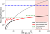 |
Fig. 12 Dispersive and scattering smearing time as a function of the DM. The black line represents the intra-channel dispersive smearing. The red lines correspond to the intra-subband dispersive smearing. The dashed green lines indicate the used time sampling. On the top, the dotted black line shows the average scatter broadening, and the blue line indicates the median of the period of all the non-MSPs in the ATNF catalogue. The pink area marks the DMs not searched for in the NPBS. |
5.3.2 DM step
The second limit value to determine was the DM step. Using the precise dispersion relation in Eq. (1) rather than the linear approximation, the ideal DM step would be 5.27.10−3 pc cm−3. However, reaching 70 pc cm−3 would require 13 280 trial DMs, which represents a substantial computing time greater than ten hours per pointing. We have tested whether the DM step could be increased. For this we used the pulsar B2334+61 (J2337+6151), which was observed during a test phase using the observational setup of the NPBS; and this pulsar was one of the faintest pulsars redetected during this phase test.
The search for B2334+61 was carried out using several DM steps between 5.27.10−3 and 0.1 pc cm−3. The pulsar was detected until 0.01 pc cm−3 . As a result, the DM step used for the NPBS has been set to 0.01 pc cm−3, representing only two times the minimum DM step but still allowing to reduce the computing time by a factor of two.
For most surveys, the DM step increases with increasing DM. However, because of the high sensitivity to the DM below 100 MHz, this DM step of 0.01 pc cm−3 was considered the largest reasonable DM step for the NPBS. Accordingly, a fixed DM step of 0.01 pc cm−3 is used for the whole DD plan.
5.3.3 Definition of the DD plan
The dedispersion of data is realised using PREPSUBBAND from PRESTO. It permits us to perform efficient dedispersion by grouping trial DMs having identical parameters of downsampling, number of subbands, and DM step.
Because there is a significant difference in the smearing time between the top and bottom of the bandwidth, the downsampling and the number of channels to group in a subband have to be computed for the lowest frequency channel. Based on the precise dispersion relation, the downsampling factor ds can be calculated for a given DM using:
 (12)
(12)
Here, ν0 represents the lowest frequency of 39.25 MHz, and tsamp is the initial time sampling of 10.485 ms. Inversing the relation, one finds that a value of ds = 2 should be used for DMs above 50.06 pc cm−3 .
Also, using the same relation, we can determine the DM where the use of subbands is possible. For a subband width of two channels, the intra-subband smearing is longer than the initial time sampling for DMs above 25.03 pc cm−3 . We can thus define three regimes: the low-DM regime (below ~25 pc cm−3 , where we can rebin in the frequency dimension, the mid-DM regime (between ~25 and ~50 pc cm−3 ), where no rebinning is possible, and the high-DM regime (above ~50 pc cm−3), where we can rebin in the time dimension.
The number of channels nc to group in a subband was determined as the number of channels starting from the lowest channel with a dispersive smearing less or equal to the used time sampling ds ⋅ tsamp . It was thus calculated following the relation:
![Mathematical equation: ${n_c} = {{{\upsilon _0}} \over {\Delta \upsilon }} \cdot \left( {{{\left[ {1 - {{ds \cdot {t_{samp}} \cdot \upsilon _0^2} \over {{\cal D} \cdot DM}}} \right]}^{ - 1/2}} - 1} \right).$](/articles/aa/full_html/2025/01/aa46654-23/aa46654-23-eq16.png) (13)
(13)
However, following this, the number of channels (and then the number of subbands) would need to change seven times for DMs lower than 8 pc cm−3 . This would lead to small groups of a few trial DMs at low DM and large groups of several hundreds of trial DMs at high DM. Also, because the subbands are smaller, the low DMs are faster to dedisperse than the high DMs. Consequently, the dedispersion carried out by PREPSUBBAND would be not homogeneous.
For each group of trial DMs, PREPSUBBAND dedisperses the data taking the minimum DM, the DM step, and the number of trial DMs as input parameters. In order to optimise the computing time, the dedispersion was realised with a multiprocessing scheme working on groups of 431 trial DMs simultaneously, leading to changes of processing parameters (ds and Nsubb) at slightly different DM values when compared to those calculated above.
The final DD plan is presented in Table 3. Each line corresponds to a group of trial DMs dedispersed using the same downsampling factor ds and number of subbands Nsubb. The last column indicates the intra-subband dispersive smearing in the lowest subband for the largest DM of the range. In total, 6896 trial DMs are tested from 1 to 69.96 pc cm−3, with dedis-persion performed channel by channel in the range of 22.55–69.96 pc cm−3. In Fig. 12, the dispersive and scatter smearing times are plotted as a function of the DM (solid and dotted black lines). These lines correspond to the maximum smearing computed in the lowest frequency channel. Also, for every line of the DD plan, the pulse broadening due to the intra-subband dispersion is shown in red (corresponding to the maximum dispersive smearing in the lowest frequency subband).
Although the optimisation is not perfect with respect to the number of subbands for each integration value, the computing time is managed efficiently by starting the processing of a new dataset once a sufficient number of CPUs becomes available. Using this DD plan and a multiprocessing structure, the dedispersion represents 71% of the total computing time per pointing with an average CPU load of 89% of the processing node.
Dedispersion plan used for the NPBS.
5.4 Periodicity search
The dedispersion step provides a time series integrated with observing frequency per DM. It allows us to search for periodic signals such as those expected for regular pulsars (as opposed to rotating radio transients – RRATs – or nulling pulsars, which require a different type of processing, see Sect. 5.8). For each dedispersed time series, the FFT is computed using REALFFT of PRESTO and the birdies (see Sect. 5.2) are zapped using ZAPBIRDS of PRESTO too.
For each produced FFT power spectrum, we use ACCELSEARCH to identify the Fourier frequencies whose significance exceeds a given threshold. The significance is calculated as the Gaussian equivalent of the chi-square probability for the power level detected at this frequency to be caused by noise. Because most of the pulsar spectra seem to decrease below 100 MHz, we expect pulsars with low S/N when compared to higher frequency surveys. Hence, the threshold was set to 2σ. A small error in the DM causes a decrease in the S/N of the pulsar in the time series. Nevertheless, whether the S/N at the ideal DM is sufficiently high, the signal can be detected in the neighbour DMs with a lower significance. As a result, although 2σ corresponds to a rather low Gaussian probability, it permits us to identify a potential pulsar signal in several neighbour DMs. This property is important for the subsequent step of the sifting (see Sect. 5.5).
Because of our coarse sampling time of 10.485 ms, short-period pulsars, such as millisecond pulsars, are very difficult or even impossible to detect. As a result, only Fourier frequencies corresponding to a period greater than 30 ms are retained. Although 30 ms only represents a few time samples, this allows us to potentially detect short-period pulsars with a small scatter broadening.
At the opposite end, until recently, the slowest known pulsars were X-ray pulsars featuring periods slightly above 11s (Dib & Kaspi 2014). However, since then, the LOTAAS survey has discovered the pulsar J0250+5854. With a period of 23.5 s, this was the slowest known pulsar at the time of its discovery (Tan et al. 2018). Moreover, based on the results of the LOTAAS survey, we expect slow pulsars (i.e. with a period ≥ 1 s, Sanidas et al. 2019) to be over-represented in low-frequency pulsar surveys compared to the known population. Thereby, we extended the pulsar search up to pulse periods of 30 s8.
Because of the low period resolution at low Fourier frequencies, an FFT-based search is not perfectly suitable for searching for slow pulsars. To overcome this, we plan to later implement another search method based on a fast-folding algorithm (Morello et al. 2020). Because it is based on direct folding rather than a Fourier transform, there is no loss in period sensitivity, providing better results for long periods.
To increase the sensitivity of the search for periodic signals, ACCELSEARCH uses the incoherent harmonic summing method (Taylor & Huguenin 1969). The method consists of stretching the Fourier transform by a factor of two, and then adding the stretched series to the initial series. This way, the first harmonic is added to the fundamental frequency, allowing it to increase its amplitude. The process can then be iterated. The amplitude of the fundamental period is increased while there are harmonics still detectable at higher Fourier frequencies. Nevertheless, it is to be noticed that the sensitivity can decrease for pulsars with a large duty cycle when too many harmonics are summed (see Ransom 2001, for more details). However, the duty cycles of potential discoveries are unknown.
Moreover, a type of expected pulsars to discover is slow pulsars. In the FFT, their frequencies appear in the low Fourier frequencies where the period sensitivity is lower, that is, the difference between the periods corresponding to two consecutive Fourier frequencies is large. Hence, for slow pulsars, the initial significance of the fundamental harmonic can be relatively low and the harmonic summing can be useful. Consequently, we summed Fourier frequencies up to 32 harmonics.
In addition to the identification of major Fourier frequencies, ACCELSEARCH can also perform an acceleration search to find accelerated periodicities (Ransom et al. 2002). In the case of acceleration, a pulsar exhibits a periodic drift of its period over time, resulting in a broadening of the signal in the FFT.
These accelerated periodicities correspond indeed to pulsars moving in a binary system. However, this search for accelerated periodicities requires a significant amount of computing time. Furthermore, according to the ATNF catalogue, the population of known pulsars in a binary system having a period longer than 30 ms merely represents about 2% of the whole population. The search for accelerated periodicities is therefore not carried out and solely isolated pulsars are searched. Nonetheless, an acceleration search could be included in a future reprocessing of the survey data.
5.5 Sifting of the candidates
For each trial DM, ACCELSEARCH produces the list of FFT candidates found in the time series. Thus, the same FFT candidate may appear in several lists. To obtain a unique list of the candidates present in the pointing, all the candidate lists are compared and combined using the python script ACCEL_SIFT.PY of PRESTO. Taking some selecting parameters as input, it aims to identify the redundant FFT candidates to provide a shorter list of candidates.
Therefore, FFT candidates corresponding to different harmonic frequencies are removed, keeping solely the one with the highest significance as the fundamental period. Similarly, for FFT candidates with the same period appearing at different trial DMs are removed, keeping solely the one with the best significance.
Also, as mentioned in Sect. 5.4, a pulsar signal must appear in several neighbour DMs. The closer the trial DM is to the true value, the higher the S/N in the time series, resulting in a higher significance of the FFT candidate. To be considered as a potential pulsar signal, we require an FFT candidate to be detected at the same period in several consecutive DMs. On the entire bandwidth used by the NPBS, the error due to our DM step of 0.01 pc cm−3 (see Sect. 5.3) produces a time delay of one time sample. Thereby, in the case of faint pulsars, the S/N of the signal can rapidly decrease relative to the DM error. As a result, the number of consecutive DMs to see the FFT candidate is only set to the minimum value of two, and candidates solely appearing in one DM value are removed.
Finally, a list of plausible candidates is generated. For each candidate, its period and DM are those of the FFT candidate having the highest significance. Also, because the search for periodicities aims to detect a signal at several DMs, the threshold used for ACCELSEARCH for the significance was set to a low value of 2σ (see Sect. 5.4). However, for the sifting, the final selected candidates need to correspond to a low probability of being a noise. Consequently, only candidates with a significance greater than 5σ are retained for the folding step.
5.6 Folding of the candidates
The list of candidates generated by ACCEL_SIFT.PY only provides periods and DM values. Then, in order to check if the candidate is a potential pulsar signal, the data (after flattening and RFI cleaning) are dedispersed and folded taking the period and DM of the candidate as input parameters.
This step is carried out using PREPFOLD of PRESTO. In addition, PREPFOLD allows us to perform a fine search for three parameters: the DM, the period, and the period derivative. The DM and period searches are realised around the input-given values. The search for the period derivative is realised around 0 s s−1. Finally, more precise values of the period and DM are provided (with an approximative value of the period derivative), and a new significance is calculated by PREPFOLD based on the more accurately folded and dedispersed data. Also, a resulting figure is generated showing eight subplots: the integrated profile, the time-phase diagram, the frequency-phase diagram, the evolution of the χ2 as a function of the DM, the evolution of the χ2 as a function of the period, the evolution of the χ2 as a function of the period derivative, and the period-period derivative plane of the χ2.
The computing time required by PREPFOLD depends on the number of trial values for the fine searches. Also, the number of trial values depends on the number of bins (in time and frequency) to dedisperse and fold. The number of candidates selected by the sifting step is of the order of 100 candidates per pointing. Consequently, the input parameters were determined for each candidate individually in order to have proper fine searches while constraining the computing time.
For the folding and the dedispersion, data are divided into time sub-integrations and frequency subbands. The length of the sub-integration is determined to correspond to 50 periods of the candidate. Also, the number of sub-integrations is constrained to a range from 8 to 32. The maximum number is defined to limit the computing time. The minimum value is set to obtain a sufficient number of points for further analysis of the folded candidate.
The number of channels in a subband is calculated using a relation similar to Eq. (13). The difference is that here, the size of the frequency subband is determined such that the dispersive smearing is shorter than a quarter of the period of the candidate in the lowest subband. Because of the large number of candidates to dedisperse and fold, the use of subbands rather than channel by channel was chosen to save a significant amount of computing time. Furthermore, PREPFOLD was tested on test data of known pulsars. Although the dedispersion by channel might be more precise, results were not noticeably better than those using subbands, providing similar significances by PREPFOLD.
For the fine searches, the ranges of trial values were determined in order to obtain a sufficiently large plot of the evolution of the χ2 of the profile to clearly distinguish the peak and the baseline. Accordingly, the DM range was set to ± 1 pc cm−3 around the initial DM value and the period range to ± 0.2% of the initial period. For the entire observing duration of 30 min, such a period error produces a cumulative error of about 3.6 s. Although it is very large for a short-period potential pulsar, for one with a period of 30 s (the longest period searched), that represents merely about 12% of its period. In the same way, the DM error of ±1 pc cm−3 represents a dispersion smearing in the entire bandwidth of about 4 s, corresponding to 13% of a period of 30 s.
For the time resolution of the profile, the initial resolution of 10.485 ms was kept as much as possible. However, the number of samples in the profile is a parameter defining the number of trial periods and DMs to perform, and thus the computing time. Hence, the time sampling was increased in order to have a total number of trial values (for the period, period derivative, and DM) smaller than one billion.
5.7 Candidate classification
66% of the pointings of phase one of the NPBS observations (see Sect. 3.5) are processed, corresponding to a third of all. In this first third, 137 200 candidates were found by the search pipeline and then folded by PREPFOLD. This number of candidates is too large to be checked manually. A sorting algorithm has been developed in order to reject as many bad candidates as possible. This ordering is based on the comparison of the candidate’s data generated by PREPFOLD with pulsar models using Monte-Carlo simulations. It is performed in a subsequent stage following the processing, which reduces the number of candidates from 137 200 initial candidates to 5245 top candidates, which then have to be checked manually. The method is described in detail in Brionne (2023) and will be presented in a future publication.
List of the seven known pulsars redetected by the NPBS.
5.8 Single pulse search
In addition to the periodicity search, we also carry out a search for single pulses on each dedispersed time series. This different analysis could allow us to identify non-periodic orquasi-periodic transients such as RRATs, pulsars with nulling, or extremely slow pulsars which would be difficult to find in 27-minute observations using an FFT-based method.
The search is realised using the Python software SINGLE_PULSE_SEARCH.PY from PRESTO, modified to allow multiprocessing computing. To identify the single pulses in the dispersed time series, an S/N threshold of >5σ is used.
The analysis of single pulse search results will be analysed in parallel with the periodicity search results using a deep learning method. This analysis will be presented in a subsequent article.
6 Results
A validation stage of the search pipeline has been realised to evaluate the possibilities of detection of the NPBS. This stage was based on the results of the first pulsar catalogue of NenuFAR realised by the NenuFAR pulsar census (Bondonneau et al., in prep.). The validation consists of searching pulsars known to be detectable by NenuFAR (i.e. detected by the NenuFAR census) in the already processed pointings of the NPBS.
Compared to the NPBS, the pulsar census observations were carried out with a larger number of NenuFAR mini-arrays, using the precise coordinates from the ATNF catalogue, and with a different observing duration and bandwidth. Moreover, data were dedispersed and folded using the precise characteristics (period, DM, etc) of the NenuFAR ephemerides. Accordingly to these differences, except in the case of more favourable scintillation, the S/N obtained by the census must be larger than that of the NPBS. To estimate the S/N potentially expected by the NPBS, the S/N from the census has been corrected for the differences in bandwidth and duration. Also, because pointings are not pointed towards the pulsar (as opposed to the census), a correction for the loss in sensitivity due to the distance between the centre of the digital beam and the pulsar’s position is applied. The loss of S/N has thereby been estimated using a Gaussian approximation of the beam. The Gaussian allows us to model the main lobe of the digital beam, where the edge of the digital beam is localised at the FWHM of the Gaussian, corresponding therefore to a loss of 50% of the S/N at the centre. On average, the simple Gaussian approximation only deviates by 1.4% from the more complex beam model generated with NenuPy at the central frequency.
The NenuFAR pulsar census has detected 54 pulsars above 39° of declination. For each pulsar, because the currently processed data only belong to observations from phase one, the closest pointing of phase one was identified. For 24 of them, the closest pointing was processed, and the corresponding pulsar was searched in the list of candidates provided by PRESTO. Folded candidates with a DM closer than 1% of the DM of the searched pulsar are selected as good matching candidates. For these selected candidates, in order to identify harmonics, the ratio between the periods of the candidate and the pulsar is calculated. Finally, the folded candidates with a period ratio corresponding to a harmonic of the pulsar were manually checked.
Some pulsars are indeed closer to a pointing from phase two, resulting in a substantial loss of S/N compared to the census. In these cases, the detected flux is divided by more than a factor of two compared to the potential flux for a beam targeted at the pulsar, significantly reducing the probability of detection. The majority of the 24 pulsars searched are actually in this situation: Only 10 are located in a pointing from phase one and 14 in a pointing from phase two.
6.1 Known pulsars redetected
In all the folded candidates of the 24 pointings, 32 candidates finally match with the pulsar expected to be present in the pointing. These candidates correspond to diverse harmonics of seven bright pulsars, representing about 29% of the 24 pulsars. The seven redetections are shown in Figs. A.1–A.7. They are also listed in Table 4, providing a comparison between the characteristics of the pulsar according to the ATNF catalogue and those of the best-found folded candidate. The last four columns present the ideal S/N (S/N0 in the table), the angular separation from the centre of the digital beam, and the expected S/N due to the angular separation between the pulsar and the beam centre. The last column indicates the significance calculated by PREPFOLD after the folding of the candidate. Comparing the two last columns, one can note a good correlation between the expected S/N and the significance.
Of the initial list of 24 pulsars, the six pulsars with the highest expected S/N are well detected with the six highest significances. As for the seventh detected pulsar, B1811+40 (J1813+4013) is the faintest detection of the seven pulsars. Also, it was merely ordered at the 12th position in the initial list of pulsars. In addition, its angular separation of 0.757° from the beam centre indicates that the pulsar is outside the limit of the beam of −3 dB (see Sect. 3.2), meaning that the closest pointing is indeed a phase two pointing. We can therefore presume its detection is due to an increase of the flux due to scintillation during the NPBS observation compared to the census observation.
It should be noted that B0655+64 (J0700+6418) was detected at a different period compared to the one given in the ATNF catalogue. The best candidate found by ACCELESEARCH corresponds indeed to the third harmonic, that is, the harmonic with a period three times longer. Although the fundamental harmonic was also detected, the third one appeared with a larger Fourier power and was considered as the fundamental period by ACCELSEARCH. Nonetheless, after manual checking of the folded candidate, the shape of the integrated profile does correspond to that of the pulsar B0655+64 as obtained in the NenuFAR pulsar census.
6.2 Baseline variations
On the plot of the integrated profile of B0809+74 in Fig. A.3, one can see the baseline around the pulse is not flat. This behaviour can also be seen for B1112+50 (Fig. A.4), B1508+55 (Fig. A.5), and B1839+56 (Fig. A.7), but with a smaller amplitude. For the three other redetections, the baseline appears flat.
The variation with dips around the pulse can be explained by the flattening in time realised in Sect. 5.1. The flattening of the time series is carried out using a running average. Thus, for bright pulsars whose single pulses can be detected without folding, the value of the running average is increased at any point where a pulse appears in the window of the calculus. To reduce the edge effects caused by the discontinuities of the time series (see Sect. 5.1 for the details), the chosen window is Gaussian.
The flattening consists of subtracting the running average from the initial time series. Consequently, a dip will appear in the area around every single pulse. However, the amplitude of the dip is proportional to the amplitude of the pulse compared to the baseline. Dips can therefore only appear for the brightest pulsars. According to Table 4, B0809+74 is indeed the strongest redetected pulsar. Also, the three pulsars without any dips are the three less bright of the redetections.
Ultimately, the baseline variations only occur for the brightest pulsars with single pulses of large amplitude. Also, when the ON-pulse is shorter than the window size of 1.845 s, the running average stays sufficiently close to the value of the OFF-pulse to not erase the single pulses. However, according to the ATNF pulsar catalogue, the pulsar with the widest pulse at 10% of the maximum amplitude is J1503+2111 with a width of 1.272 s (Posselt et al. 2021). As a consequence, except for the case of a bright pulsar with an uncommon very wide pulse, faint pulsars are not affected and the pulses of bright pulsars are still detectable by the search process.
Known pulsars not detected during the validation stage.
6.3 Non-detections
17 pulsars potentially present in a processed pointing have been not detected. They are listed in Table 5, indicating their characteristics (from the ATNF catalogue), their angular separation from the centre of the closest digital beam, and their expected S/N. Two of these are impossible to detect because of a period shorter than our sampling time. Also, two others have a period of approximately 40 ms. Although this is longer than the NPBS sampling time, they must be very difficult to detect. In addition, these two pulsars have extremely low expected S/N of 2.4 and 1.0. Of the 13 remaining pulsars, eight have an expected S/N ≤ 3.8. It is lower than 4.8 which is the expected S/N of the faintest known pulsar detected: B1811+40 (see Table 4). Hence, we can assume they are below our detection limit.
Finally, five not detected known pulsars should have an S/N greater than 4.8. However, two of them, namely J1343+6634 and J0742+4334 are clearly outside the digital beam. This leaves three pulsars for which we might have expected a detection in the NPBS.
These remaining pulsars are B0917+63 (J0921+6254), J1426+52 and J1647+6608 with expected S/Ns respectively of 5.3, 5.2, and 6.1. Although B0917+63 is located on the edge of its digital beam, they could theoretically be detected. However, in addition to the distance from the centre of the digital beam, there are other differences between a standard pulsar observation and an observation in search mode which are not taken into account in the determination of the expected S/N. In the case of the Nen-uFAR pulsar census, the S/N is computed from an observation processed with a coherent intra-channel dedispersion and folding of the pulsar using a precise ephemeris. In the case of the NPBS, although our data should be insensitive to the intra-channel dispersion because of the chosen time and frequency resolutions (see Sect. 4.1), the folding is realised using a less precise folding technique. More importantly, this folding is carried out on data with a coarse time sampling of about 10 ms, resulting in a less precise profile compared to a standard pulsar observation.
Finally, another effect (independent of the observation setup and of the processing technique) can explain the difference in S/N compared to the expected S/N. The S/N can vary due to refractive scintillation, which is related to the movement of the line-of-sight with respect to scattering screens at large scales. The resulting increase or decrease of the S/N is a function of the sky position, that is different for each pulsar, and of time. As a consequence, one can suppose the non-detection of these three pulsars compared to B1811+40 can be attributed either to a decrease in their flux at the time of the observation or, on the contrary, to an increase in the flux of B1811+40 (compared to its observation in the pulsar census) during its NPBS observation.
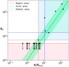 |
Fig. 13 Significance provided by PREPFOLD relative to the corresponding expected S/N. The green area indicates the values of supposed sure detectability by the NPBS. The light blue area marks values for which the detection is possible depending on scintillation. The red area represents the values for which a pulsar candidate is rejected by the search pipeline (Sσ < 5σ). The green diagonal contour represents the slope 1 between the significance and the expected S/N, with an error bar of factor 2. |
7 Discussion
Although there are no discoveries, the known pulsars detected and not detected provide us information about the capacities of detection of the NPBS. Using this, it is possible to derive an estimate of the detection limits of the NPBS in terms of significance, S/N, DM, or period.
7.1 Estimation of the detection limits
Based on the expected S/N for the seven detections (column seven in Table 4), a first estimation of the lowest S/N required to be detected by the search pipeline can be determined. Also, using the corresponding significances computed by PREPFOLD (column eight in Table 4), the lowest significance where a pulsar signal must appear can be estimated.
Figure 13 shows the significance Sσ provided by PREPFOLD as a function of their expected S/N. The seven detections are represented by the black squares. Also, the 17 non-detections are indicated by upper limits in significance. Because they are not detected, the significance given by PREPFOLD is unknown. However, the non-detection means that the Fourier power of the pulsar is lower than the threshold of 5σ required for the sifting step (see Sect. 5.5). Thus, as a first approximation, we can assume that these pulsars have a significance between 0 and 5σ.
The faintest known pulsar detected is B1811+40 and it can be used to determine the detection limits. Thereby, the lowest significance obtained by a pulsar signal must be greater or equal to 6.9σ. Also, the NPBS could detect only pulsars having an S/N greater or equal to 4.8.
However, five pulsars are not detected even though their S/N is larger than 4.8; these two limit values thus cannot be considered as absolute limits. Scintillation seems to be the most likely explanation of the detection or not of pulsars with expected S/N around a value of 5. In Fig. 13, the grey lines indicate the minimum value of S/N and significance, and the light blue area marks the area for which the detection is possible but depends on the scintillation at the time of the observation.
The largest expected S/N of the non-detections is 6.1 (J 1647+6608 in Table 5). All pulsars with an expected S/N greater than this value have been detected. The detected pulsar with the lowest S/N greater than 6.1 is B1112+50 (with S/N = 11.1). Then, we can suppose all pulsars having a S/N greater or equal to 11.1 could be detected. In the same way, except B1811+40, the pulsar with the lowest significance is B0655+64. We can equally therefore assume that a detectable pulsar signal must obtained, after folding by PREPFOLD, a significance greater or equal to 14.1σ. This area of supposed sure detectability is indicated by the green area at the top right of the graph. This area is delimited by the two blue lines corresponding to the expected S/N of B1112+50 and the significance of B0655+64.
Finally, the red area at the bottom of Fig. 13 indicates the rejection area below 5σ. According to the threshold of 5σ used for the sifting of the FFT candidates (see Sect. 5.5), all pulsar signals with a significance less than 5σ are then rejected. The significances plotted in Fig. 13 are those provided after the folding of the filterbank file by PREPFOLD. It is, in principle, possible for an FFT candidate with a significance provided by ACCELSEARCH greater than 5σ to have a smaller final significance after folding. Nevertheless, for a pulsar signal, the folding performed by PREPFOLD, including a fine search of the period, DM, and period derivative, needs to increase the signal. It is therefore unlikely a pulsar signal has a significance (after folding) below 5σ.
7.2 Flux density limits and the sensitivity of the NPBS
Using the radiometer equation (Dewey et al. 1985) with the observing parameters provided in Table 2, two minimum flux densities can be roughly estimated based on the two limits in expected S/N (i.e. 4.8 and 11.1). At NenuFAR frequencies, the sky temperature is considerably larger than the telescope temperature, leading to the system temperature being almost equal to the sky temperature. According to the sky temperature map of Haslam et al. (1982), calculated at the central frequency of the NPBS of 58 MHz with an average spectral index of −2.6 (Lawson et al. 1987), the sky temperature varies by a factor of 50 from about 3 000 K in the coldest sky regions to 155 000 K in the direction of the Galactic centre.
Figure 14 shows two sky maps of the minimum flux density required for pulsar detection. Based on these sky estimations, each map is computed for a typical duty cycle of 0.1 and a gain of 1.55 K Jy−1. Thereby, depending on its location, a pulsar needs to have a flux at 58 MHz from 14.11 mJy in the coldest regions to 5220 mJy in the hottest regions to be surely detected (i.e. to obtain an S/N greater than 11.1). Also, depending on scintillation during the observation, a pulsar can potentially be detected whether its flux is greater than a value ranging from 6.10 mJy in the coldest regions to 2260 mJy in the hottest regions.
Except for two pulsars, one can notice on the maps that all the searched pulsars are off the Galactic plane in rather cold regions. The two pulsars localised close to the plane are B0450+55 (which is detected) and J0518+5125 (not detected) with Galactic latitudes of 7.5° and 7.9°. Nevertheless, they are far from the Galactic centre with Galactic longitudes of 152 and 158°. The regions for both are actually relatively cool with temperatures of about 6600 and 6000 K, which is in the lower part of the temperature range from 3000 to 155 000 K. Also, in the region around B0450+55, the minimum flux density is evaluated at 45 mJy, and it was detected in the LOFAR-LBA pulsar census (Bilous et al. 2020) with a mean flux of 110 ± 60 mJy between 42 and 76 MHz. On the contrary, J0518+5125 was not observed as part of the two LOFAR LBA pulsar studies (Bilous et al. 2020; Bondonneau et al. 2020). It was, however, marginally detected by NenuFAR (see Bondonneau et al., in prep.), consistent with the non-detection in the NPBS.
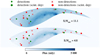 |
Fig. 14 Maps of the NPBS flux sensitivity for the sky above 39° of declination in the ecliptic frame. Top: flux map corresponding to the minimum expected S/N for sure detection. Bottom: flux map corresponding to the minimum expected S/N for detection depending on the scintillation effect. Green diamonds represent the detected known pulsars and red crosses the not detected known pulsars. Pulsars marked by a circle correspond to those with an expected S/N between 4.8 and 11.1. |
7.3 Detection of binary pulsars
One of the seven detections, B0655+64 has the particularity to be a binary pulsar with an orbital period of 24.68807286(2) h (Jones & Lyne 1988). Also, it is the only one for which the best candidate found by ACCELSEARCH does not correspond to the fundamental period, but to a harmonic.
In order to evaluate whether the binarity can disturb the detection, an acceleration search was performed using ACCELSEARCH searching periodicities with a drift up to ten Fourier frequency bins. Similarly to the standard periodicity search, B0655+64 is not detected for a period corresponding to its fundamental period. It is indeed detected for a longer period of 978.61 ms, corresponding to the harmonic five. We can conclude from the detection of B0655+64 that, although there is not any acceleration search, the NPBS can potentially detect some binary pulsars, provided that they have a sufficiently long enough orbital period.
7.4 Detectable periods
From our seven redetections, the fastest-spinning pulsar is B0655+64 with a spin period of 195 ms. Although the final candidate found by ACCELSEARCH corresponds to the harmonic three, the fundamental period is well detected. The FFT candidate corresponding to the fundamental period is detected with a significance computed by ACCELSEARCH of 7.7σ. It is thus greater than the limit of 6.9σ (see Sect. 7.1), resulting in the possibility of detecting a potential pulsar of 195 ms.
Furthermore, of the 32 folded candidates corresponding to a known pulsar, many of them are harmonics with a period shorter than 195 ms. The folded candidate with the shortest period has a period of 38.98 ms and corresponds to the harmonic 20 of the pulsar B1508+55 (J1509+5531). This folded candidate is clearly detected with a significance of 11.6σ given by PREPFOLD.
On the opposite side, the pulsar with the longest period is B1112+50 with a period of 1.65644 s. Nonetheless, as in the case of the short periods, many folded candidates corresponding to harmonics of longer periods have been found. The folded candidate with the longest period is the harmonic 14:3 of B1508+55 with a period of 3.44709 s. Also, this candidate was easily detected by the search pipeline, PREPFOLD providing a final significance of 60.70σ. Consequently, from these different detections, we can estimate the range of detectable periods is at least from 40 ms to ~3.5 s.
7.5 Highest detectable DM
The detected pulsar with the highest DM is B1811 +40 with a DM of 41.557 pc cm−3. It should be noted that B1811+40 is weakly scattered at the NenuFAR frequencies (Bondonneau et al., in prep.). According to the detection realised by the census, the scatter broadening increases the pulse width to approximately 10% of its period. From this detection, we can estimate that pulsars with DM values lower than 42 pc cm−3 can be detected.
However, it should be noted this DM limit, as well as the range of periods, is determined based on a small set of detection of merely seven pulsars. Moreover, in the set of the 24 pulsars detected by the census, B1811+40 is the pulsar with the highest DM. As a result, the DMs between 41 and 70 pc cm−3 could not be tested. We expect to refine these values of DM and period as soon as further data will be processed.
8 Summary and conclusion
The NPBS is an all-sky survey using NenuFAR, aiming to discover new pulsars at low frequencies in the range of 10–85 MHz. Contrary to previous surveys at higher frequencies, we expect to especially find pulsars with steep spectra or pulsars localised in unusual parts of the P − Ṗ diagram such as slow pulsars close to the pulsar death line. The difficulty of low-frequency surveys is to deal with high dispersion, strong scattering, and significant long-term scintillation of the measured pulsar flux. Moreover, it seems that most of the pulsars possess a spectral turnover at a low frequency, reducing their flux density. Nevertheless, certain pulsars could be solely detectable at very low frequencies due to a potential widening of the emission cone or birefringence of the emission within the pulsar magnetosphere.
To evaluate the potential discoveries of a low-frequency survey such as the NPBS, three different types of simulations have been carried out. Firstly, a population synthesis using PSRPOPPY has been realised. In order to adapt to low frequencies, the possibility of spectral turnover has been included, and expected discoveries were determined by adding the LOTAAS survey to the series of previous surveys. The simulation finally gives us 70 ± 9 detections and 2 ± 2 discoveries for the NPBS.
Secondly, the modelling of the emission cone size relative to the observing frequency, the period and the period derivative of the pulsar has been realised based on the RFM. Including the constraint of scattering, we can expect to discover up to 8 pulsars localised in the centre part of the P − Ṗ diagram, and one slow pulsar localised in the right part of the P − Ṗ diagram, for the observations of the first stage of the NPBS (declination above 38.7°).
The last simulation is a Monte-Carlo simulation of pulsar spectra with and without spectral turnover. Using the LOTAAS survey parameters, the most probable discoveries of the NPBS should be: (a) pulsars without any spectral turnover and a spectral index around 3.2; (b) pulsars with a turnover frequency lower than ~60 MHz, and spectral indices around 3.4 at high-frequency and 0.5 at low-frequency.
The population synthesis has the advantage of generating a realistic base population. However, it is based on discoveries from higher frequency surveys, which do not necessarily have the same characteristics as at lower frequency. On the opposite, the modelling of the widening of the emission cone allows for adapting to low frequencies. However, the number of potential discoveries is provided in the case of similar pulsar flux and survey sensitivity between the studied and reference surveys. These two approaches could be merged to obtain frequency variations according to a model of emission cone. For the Monte-Carlo simulation of spectra, the advantage is to extend the pulsar population, reaching the less probable parts of the parameter space. Nevertheless, the modelled population may be not realistic. The population synthesis could be thus combined with the Monte-Carlo approach to probe the parameter space by varying the parameter distributions and models.
The NPBS aims to observe the entire sky visible by NenuFAR, that is, above −23° of declination. The observing programme presented in this work is indeed the first stage. The northern sky between 38.7° of declination and the northern polar cap is observed using a grid of 7692 pointings spaced by 0.98° with a diameter of approximately 1.47°. The average beam surface is 1.69 deg2, allowing us to observe 98.4% of the targeted sky with a minimum covering of 90.2% at the highest frequency. Each pointing is observed during nighttime with a duration of 27 minutes with a time sampling of 10.485 ms. The observation is performed using a bandwidth of 37.5 MHz around the central frequency of 58 MHz and a high-frequency resolution of 1.52 kHz, allowing to limit the impact of intra-channel dispersion.
The observations of the NPBS as described above started in August 2020, and are expected to be completed during 2024. Future extensions (to increase the sky coverage to declination ranges below 39°) are planned in the next years.
Data are reduced to the total intensity and processed using a search pipeline based on the software PRESTO, with some adaptations to the constraints of NenuFAR and low frequencies. Regular pointing adjustments of NenuFAR create discontinuities of the time series, disturbing the RFI mitigation. A first step for flattening the time series using a running average by Gaussian convolution combined with rough mitigation of the major RFIs is carried out beforehand of the standard RFI mitigation flagging signals >3σ. Because of the significant intra-channel dispersion at the NenuFAR frequencies, a dedispersion plan based on the exact dispersion within the lowest frequency channel has been defined rather than using the usual diagonal DM method. The search for DM is realised between 1 and 70 pc cm−3 using a fixed DM step of 0.01 pc cm−3. Because of our coarse sampling time and the low probability of detecting non-recycled binary pulsars, periodicities are searched without any acceleration for signals >5σ from 30 ms to 30 s.
Following this first processing, further reprocessing is planned in order to extend the parameter space of the survey: DM searches for very low DMs below 1 pc cm−3and for higher DMs; performing an acceleration search to search for binaries; a single pulse analysis using deep learning. Also, we expect the NPBS to be particularly well adapted to detect slow pulsars and plan to implement a fast-folding algorithm.
Currently, 66% of the pointings from phase one are processed, representing 1/3 of the whole survey, and 137 200 pulsars candidates have been found. 24 known pulsars located in the processed data and detected by the NenuFAR pulsar census have been searched, leading to the detection of seven of them, including one binary pulsar (B0655+64). Six of these detections are indeed the six brightest pulsars expected to be detected by the NPBS. The last detection of B1811+40 is probably due to an increasing flux caused by the refractive scintillation. For most of the non-detected pulsars, a non-detection was indeed expected: four pulsars have very short periods; three are located outside the telescope beam; the others have a low expected S/N. Comparing to the seven detections and according to their previous detection by the census, J1426+52 and J1647+6608 should be detectable although they are faint. We can assume that their non-detections are due to a decrease in their flux caused by the refractive scintillation.
From these detections, the thresholds to detect a pulsar are of 14.1σ in significance provided by PRESTO and 11.1 in expected S/N (corrected S/N of the census). A second couple of lower thresholds can be defined to estimate a potential detection region, where actual detection would depend on the scintillation at the time of the observation. This region is delimited by a significance of 6.9σ and an expected S/N of 4.8. For the coldest regions of the sky, these expected S/N correspond to minimum flux densities of 6.10 mJy (depending on scintillation) and 14.11 mJy. On the opposite, in the hottest regions, the minimum fluxes are 2.26 Jy and 5.22 Jy. According to the parameters of the re-detections, the NPBS is able to detect periods at least from 40 ms to 3.5 s, and DMs at least up to 42 pc cm−3.
The ranges of detectability are derived from a small sample of 24 pulsars and will likely have to be adjusted once a large number of pointings will be processed, increasing the number of potential re-detections. The processing of pointings from phase two might allow an increase of the sample to 54 pulsars. Moreover, because of the high overlap between adjacent pointings, the observations of phase two are almost the same as those of phase one, shifted by half of a beam. Hence, a substantial number of the currently undetected pulsars could be finally detected either because of a location closer to the centre of a beam or because of a positive impact of the scintillation. Furthermore, the addition of a fast-folding algorithm should increase the range of periods able to be reached by detecting slow pulsars. Also, because one can expect slow pulsars to have smaller duty cycles, they might be less sensitive to scatter broadening, potentially leading to an increase in the DM range.
Acknowledgements
This paper is based on data obtained using the NenuFAR radio telescope. The development of NenuFAR has been supported by personnel and funding from: Observatoire Radioastronomique de Nançay (ORN), CNRS-INSU, Observatoire de Paris-PSL, Université d’Orléans, Observatoire des Sciences de l’Univers en Région Centre, Région Centre-Val de Loire, DIM-ACAV and DIM-ACAV+ of Région Île-de-France, Agence Nationale de la Recherche. We acknowledge the use of the Nançay Data centre computing facility (CDN – Centre de Données de Nançay). The CDN is hosted by the Observatoire Radioastronomique de Nançay in partnership with Observatoire de Paris, Université d’Orléans, OSUC and the CNRS. The CDN is supported by the Région Centre Val de Loire, département du Cher. The Nançay Radio Observatory is operated by the Paris Observatory, associated with the French Centre National de la Recherche Scientifique (CNRS). I.P.K. acknowledges the support of Collège de France by means of ‘PAUSE – Solidarité Ukraine’ and of NAS of Ukraine by a Grant of the NAS of Ukraine for Research Laboratories/Groups of Young Scientists of the NAS of Ukraine (2022-2023, project code ‘Spalakh’). We thank the anonymous referee for their useful comments which helped to improve this article.
Appendix A Result plots of the detected pulsars
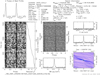 |
Fig. A.1 Result plot of the redetection of B0450+55. |
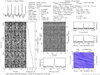 |
Fig. A.2 Result plot of the redetection of B0655+64 (harmonic corresponding to three times the fundamental period). |
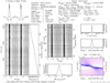 |
Fig. A.3 Result plot of the redetection of B0809+74. |
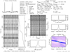 |
Fig. A.4 Result plot of the redetection of B1112+50. |
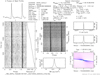 |
Fig. A.5 Result plot of the redetection of B1508+55. |
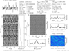 |
Fig. A.6 Result plot of the redetection of B1811+40. |
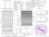 |
Fig. A.7 Result plot of the redetection of B1839+56. |
References
- Bates, S. D., Lorimer, D. R., Rane, A., & Swiggum, J. 2014, MNRAS, 439, 2893 [NASA ADS] [CrossRef] [Google Scholar]
- Bhat, N. D. R., Cordes, J. M., Camilo, F., Nice, D. J., & Lorimer, D. R. 2004, ApJ, 605, 759 [CrossRef] [Google Scholar]
- Bilous, A. V., Kondratiev, V. I., Kramer, M., et al. 2016, A&A, 591, A134 [NASA ADS] [CrossRef] [EDP Sciences] [Google Scholar]
- Bilous, A. V., Bondonneau, L., Kondratiev, V. I., et al. 2020, A&A, 635, A75 [NASA ADS] [CrossRef] [EDP Sciences] [Google Scholar]
- Bondonneau, L., Grießmeier, J.-M., Theureau, G., et al. 2020, A&A, 635, A76 [NASA ADS] [CrossRef] [EDP Sciences] [Google Scholar]
- Bondonneau, L., Grießmeier, J. M., Theureau, G., et al. 2021, A&A, 652, A34 [NASA ADS] [CrossRef] [EDP Sciences] [Google Scholar]
- Brionne, M. 2023, PhD thesis, Université Orléans, France [Google Scholar]
- Caleb, M., Heywood, I., Rajwade, K., et al. 2022, Nat. Astron., 6, 828 [NASA ADS] [CrossRef] [Google Scholar]
- Chen, J. L., & Wang, H. G. 2014, ApJS, 215, 11 [NASA ADS] [CrossRef] [Google Scholar]
- Cole, T. W., & Pilkington, J. D. H. 1968, Nature, 219, 574 [NASA ADS] [CrossRef] [Google Scholar]
- Cordes, J. M. 2002, ASP Conf. Ser., 278, 227 [NASA ADS] [Google Scholar]
- Cordes, J. M., & Lazio, T. J. W. 2003, arXiv e-prints [arXiv:astro-ph/0207156] [Google Scholar]
- Della Monica, R., De Martino, I., & De Laurentis, M. 2023, MNRAS, 524, 3782 [NASA ADS] [CrossRef] [Google Scholar]
- Deneva, J. S., Stovall, K., McLaughlin, M. A., et al. 2013, ApJ, 775, 51 [NASA ADS] [CrossRef] [Google Scholar]
- de Oliveira-Costa, A., Tegmark, M., Gaensler, B. M., et al. 2008, MNRAS, 388, 247 [NASA ADS] [CrossRef] [Google Scholar]
- Desvignes, G., Kramer, M., Lee, K., et al. 2019, Science, 365, 1013 [Google Scholar]
- Dewey, R. J., Taylor, J. H., Weisberg, J. M., & Stokes, G. H. 1985, ApJ, 294, L25 [NASA ADS] [CrossRef] [Google Scholar]
- Dib, R., & Kaspi, V. M. 2014, ApJ, 784, 37 [NASA ADS] [CrossRef] [Google Scholar]
- Ellingson, S. W., Clarke, T. E., Cohen, A., et al. 2009, IEEE Proceedings, 97, 1421 [NASA ADS] [CrossRef] [Google Scholar]
- Emmering, R. T., & Chevalier, R. A. 1989, ApJ, 345, 931 [Google Scholar]
- Faucher-Giguère, C.-A., & Kaspi, V. M. 2006, ApJ, 643, 332 [CrossRef] [Google Scholar]
- Geyer, M., Karastergiou, A., Kondratiev, V. I., et al. 2017, MNRAS, 470, 4659 [Google Scholar]
- Gold, T. 1968, Nature, 218, 731 [NASA ADS] [CrossRef] [Google Scholar]
- Goldreich, P., & Julian, W. H. 1969, ApJ, 157, 869 [Google Scholar]
- Grießmeier, J. M., Smith, D. A., Theureau, G., et al. 2021, A&A, 654, A43 [NASA ADS] [CrossRef] [EDP Sciences] [Google Scholar]
- Han, J. L., Wang, C., Wang, P. F., et al. 2021, Res. Astron. Astrophys., 21, 107 [CrossRef] [Google Scholar]
- Hankins, T. H., & Rickett, B. J. 1975, Methods Comput. Phys., 14, 55 [Google Scholar]
- Haslam, C. G. T., Salter, C. J., Stoffel, H., & Wilson, W. E. 1982, A&AS, 47, 1 [NASA ADS] [Google Scholar]
- Hewish, A., Bell, S. J., Pilkington, J. D. H., Scott, P. F., & Collins, R. A. 1968, Nature, 217, 709 [NASA ADS] [CrossRef] [Google Scholar]
- Jankowski, F., van Straten, W., Keane, E. F., et al. 2018, MNRAS, 473, 4436 [Google Scholar]
- Jones, A. W., & Lyne, A. G. 1988, MNRAS, 232, 473 [NASA ADS] [Google Scholar]
- Keith, M. J., Jameson, A., van Straten, W., et al. 2010, MNRAS, 409, 619 [Google Scholar]
- Kijak, J., & Gil, J. 1998, MNRAS, 299, 855 [NASA ADS] [CrossRef] [Google Scholar]
- Kijak, J., & Gil, J. 2003, A&A, 397, 969 [NASA ADS] [CrossRef] [EDP Sciences] [Google Scholar]
- Krishnakumar, M. A., Maan, Y., Joshi, B. C., & Manoharan, P. K. 2019, ApJ, 878, 130 [NASA ADS] [CrossRef] [Google Scholar]
- Kulkarni, S. R. 2020, arXiv e-prints [arXiv:2007.02886] [Google Scholar]
- Lawson, K. D., Mayer, C. J., Osborne, J. L., & Parkinson, M. L. 1987, MNRAS, 225, 307 [Google Scholar]
- Lazarus, P., Brazier, A., Hessels, J. W. T., et al. 2015, ApJ, 812, 81 [NASA ADS] [CrossRef] [Google Scholar]
- Liu, Y. H., Ng, C. Y., & Dodson, R. 2023, ApJ, 945, 82 [NASA ADS] [CrossRef] [Google Scholar]
- Loh, A., & Girard, J. N. 2020, AlanLoh/nenupy: nenupy 1.1.0 [Google Scholar]
- Lorimer, D. R., & Kramer, M. 2012, Handbook of Pulsar Astronomy (Cambridge: Cambridge University Press) [Google Scholar]
- Lorimer, D. R., Yates, J. A., Lyne, A. G., & Gould, D. M. 1995, MNRAS, 273, 411 [NASA ADS] [CrossRef] [Google Scholar]
- Lorimer, D. R., Faulkner, A. J., Lyne, A. G., et al. 2006, MNRAS, 372, 777 [NASA ADS] [CrossRef] [Google Scholar]
- Manchester, R. N., Lyne, A. G., Taylor, J. H., et al. 1978, MNRAS, 185, 409 [NASA ADS] [CrossRef] [Google Scholar]
- Manchester, R. N., Lyne, A. G., Camilo, F., et al. 2001, MNRAS, 328, 17 [NASA ADS] [CrossRef] [Google Scholar]
- Manchester, R. N., Hobbs, G. B., Teoh, A., & Hobbs, M. 2005, AJ, 129, 1993 [Google Scholar]
- Manchester, R. N., Kramer, M., Stairs, I. H., et al. 2010, ApJ, 710, 1694 [NASA ADS] [CrossRef] [Google Scholar]
- Maron, O., Kijak, J., Kramer, M., & Wielebinski, R. 2000, A&AS, 147, 195 [NASA ADS] [CrossRef] [EDP Sciences] [Google Scholar]
- McEwen, A. E., Spiewak, R., Swiggum, J. K., et al. 2020, ApJ, 892, 76 [NASA ADS] [CrossRef] [Google Scholar]
- Miller, M. C., Lamb, F. K., Dittmann, A. J., et al. 2019, ApJ, 887, L24 [Google Scholar]
- Morello, V., Barr, E. D., Stappers, B. W., Keane, E. F., & Lyne, A. G. 2020, MNRAS, 497, 4654 [NASA ADS] [CrossRef] [Google Scholar]
- Olausen, S. A., & Kaspi, V. M. 2014, ApJS, 212, 6 [Google Scholar]
- Pacini, F. 1968, Nature, 219, 145 [NASA ADS] [CrossRef] [Google Scholar]
- Pétri, J. 2022, A&A, 666, A5 [Google Scholar]
- Pilia, M., Hessels, J. W. T., Stappers, B. W., et al. 2016, A&A, 586, A92 [NASA ADS] [CrossRef] [EDP Sciences] [Google Scholar]
- Pilkington, J. D. H., Hewish, A., Bell, S. J., & Cole, T. W. 1968, Nature, 218, 126 [NASA ADS] [CrossRef] [Google Scholar]
- Posselt, B., Karastergiou, A., Johnston, S., et al. 2021, MNRAS, 508, 4249 [NASA ADS] [CrossRef] [Google Scholar]
- Rankin, J. M. 1993, ApJ, 405, 285 [Google Scholar]
- Rankin, J. 2022, MNRAS, 514, 3202 [NASA ADS] [CrossRef] [Google Scholar]
- Ransom, S. M. 2001, PhD thesis, Harvard University, Massachusetts, USA [Google Scholar]
- Ransom, S. M., Eikenberry, S. S., & Middleditch, J. 2002, AJ, 124, 1788 [Google Scholar]
- Rickett, B. J. 1969, Nature, 221, 158 [NASA ADS] [CrossRef] [Google Scholar]
- Rickett, B. J., Coles, W. A., & Bourgois, G. 1984, A&A, 134, 390 [NASA ADS] [Google Scholar]
- Romani, R. W., Narayan, R., & Blandford, R. 1986, MNRAS, 220, 19 [NASA ADS] [Google Scholar]
- Sanidas, S., Cooper, S., Bassa, C. G., et al. 2019, A&A, 626, A104 [NASA ADS] [CrossRef] [EDP Sciences] [Google Scholar]
- Sieber, W. 1973, A&A, 28, 237 [NASA ADS] [Google Scholar]
- Tan, C. M., Bassa, C. G., Cooper, S., et al. 2018, ApJ, 866, 54 [NASA ADS] [CrossRef] [Google Scholar]
- Taylor, J. H., & Huguenin, G. R. 1969, Nature, 221, 816 [NASA ADS] [CrossRef] [Google Scholar]
- Thorsett, S. E. 1991, ApJ, 377, 263 [NASA ADS] [CrossRef] [Google Scholar]
- Tiburzi, C., Jackson, B. V., Cota, L., et al. 2023, Adv. Space Res., 72, 5287 [NASA ADS] [CrossRef] [Google Scholar]
- Tingay, S. J., Goeke, R., Bowman, J. D., et al. 2013, PASA, 30, e007 [Google Scholar]
- van der Wateren, E., Bassa, C. G., Cooper, S., et al. 2023, A&A, 669, A160 [NASA ADS] [CrossRef] [EDP Sciences] [Google Scholar]
- van Haarlem, M. P., Wise, M. W., Gunst, A. W., et al. 2013, A&A, 556, A2 [NASA ADS] [CrossRef] [EDP Sciences] [Google Scholar]
- Vasylieva, I. Y., Zakharenko, V. V., Konovalenko, A. A., et al. 2014, Radio Phys. Radio Astron., 19, 197 [NASA ADS] [CrossRef] [Google Scholar]
- Xilouris, K. M., Kramer, M., Jessner, A., Wielebinski, R., & Timofeev, M. 1996, A&A, 309, 481 [NASA ADS] [Google Scholar]
- Zakharenko, V. V., Sharykin, N. K., & Rudavin, E. R. 2005, Kinematika i Fizika Nebesnykh Tel Supplement, 5, 90 [NASA ADS] [Google Scholar]
- Zakharenko, V. V., Vasylieva, I. Y., Konovalenko, A. A., et al. 2013, MNRAS, 431, 3624 [NASA ADS] [CrossRef] [Google Scholar]
- Zarka, P., Denis, L., Tagger, M., et al. 2020, in URSI GASS 2020, Session J01 New Telescopes on the Frontier [Google Scholar]
- Zhu, Z., Li, A., Hu, J., & Shen, H. 2023, Phys. Rev. C, 108, 025809 [NASA ADS] [CrossRef] [Google Scholar]
This is not strictly true, especially below 100 MHz.
We also compared with the cutoff DM based on τsc scaling relations from Geyer et al. (2017) and Krishnakumar et al. (2019); the results are not consistent with the Census observations.
After the start of the NPBS, a pulsar with a period of 76 s has been discovered (J0901-4046, see Caleb et al. 2022). A search for such long periods in the NPBS data would require the use of a fast-folding algorithm, as described above.
All Tables
Modelling parameters of the emission cone widening and expected number of discoveries.
All Figures
|
Fig. 1 Distribution of the low-frequency parameters used for the simulations with PSRPOPPY. Left: spectral index. Right: spectral turnover frequency. |
| In the text | |
|
Fig. 2 Distribution of the numbers of discoveries and detections obtained by simulations with PSRPOPPY. The blue distribution on the left represents the number of discovered pulsars and the distribution in orange is the number of known pulsars detected for all the simulations. |
| In the text | |
|
Fig. 3 Sky map in ecliptic coordinates of the lowest spectral index required to discover a pulsar with the NPBS compared to the reference survey of LOTAAS. |
| In the text | |
|
Fig. 4 Posterior distributions for simulations using a simple power-law. Parameters are: the spectral index α, the flux at 135 MHz Flot (the central frequency of LOTAAS), and ɡl and ɡb correspond to the Galactic longitude and latitude. |
| In the text | |
|
Fig. 5 Posterior distributions for simulations using a broken power-law. Parameters are: the high-frequency spectral index αh , the low-frequency spectral index αl, the spectral turnover frequency νt, the flux at 135 MHz Flot (the central frequency of LOTAAS), and ɡl and ɡb correspond to the Galactic longitude and latitude. |
| In the text | |
|
Fig. 6 Map of NenuFAR showing the 56 mini-arrays available in 2020. Dashed red line: circle of 210 m diameter defining the sub-array used for the NPBS. Red points: the 25 mini-arrays used for the NPBS. Black points: mini-arrays not used for the NPBS. Two mini-arrays within the red circle were excluded due to high RFI levels. |
| In the text | |
|
Fig. 7 Digital beam of NenuFAR in the configuration of the NPBS modelled at the zenith for a frequency of 58 MHz. Contours represent the gain attenuation of −3 (corresponding to the FWHM of the digital beam), −6, −9, and −12 dB, respectively. White contours defining the two sidelobes around the main lobe (as well as the outer contours of the main lobe) correspond to the gain attenuation of −12 dB. |
| In the text | |
|
Fig. 8 Scheme presenting the principle of the two phases of the NPBS. Blue ellipses: pointings observed during the first phase of the NPBS. Red ellipses: pointing observed during the second phase of the NPBS. |
| In the text | |
|
Fig. 9 Stereographic projection of the observed sky month by month. Left: observations of phase one from August 2020 in red to July 2021 in purple. Right: observations of phase two from July 2021 in red to August 2022 in purple. Grey areas represent sky areas that remain to be observed. |
| In the text | |
|
Fig. 10 Intra-channel dispersion smearing at 39 MHz as a function of frequency resolution (ranging from 0.5 to 195 kHz). The five coloured lines correspond to five different DM values: (from the bottom to the top) 1, 20, 50, 70, and 100 pc cm−3 . The red dashed-dotted line corresponds to the median of the periods of all the non-MSP pulsars according to the ATNF catalogue (Manchester et al. 2005). The black dotted line corresponds to the frequency resolution of 1.529 kHz used for the NPBS and the associated smearing for the five DM values. |
| In the text | |
|
Fig. 11 Comparison of the frequency-integrated time series of an observation of the NPBS before and after the flattening step. Top panel: part of the original time series with the tracking adjustment of the analogue beam of NenuFAR just before 720 s (blue dotted line). Bottom panel: same part of the time series after the flattening step. Red dashed lines indicate the positions of the short discontinuities every 1.7 s generated during the data conversion into an 8-bit filterbank. |
| In the text | |
|
Fig. 12 Dispersive and scattering smearing time as a function of the DM. The black line represents the intra-channel dispersive smearing. The red lines correspond to the intra-subband dispersive smearing. The dashed green lines indicate the used time sampling. On the top, the dotted black line shows the average scatter broadening, and the blue line indicates the median of the period of all the non-MSPs in the ATNF catalogue. The pink area marks the DMs not searched for in the NPBS. |
| In the text | |
|
Fig. 13 Significance provided by PREPFOLD relative to the corresponding expected S/N. The green area indicates the values of supposed sure detectability by the NPBS. The light blue area marks values for which the detection is possible depending on scintillation. The red area represents the values for which a pulsar candidate is rejected by the search pipeline (Sσ < 5σ). The green diagonal contour represents the slope 1 between the significance and the expected S/N, with an error bar of factor 2. |
| In the text | |
|
Fig. 14 Maps of the NPBS flux sensitivity for the sky above 39° of declination in the ecliptic frame. Top: flux map corresponding to the minimum expected S/N for sure detection. Bottom: flux map corresponding to the minimum expected S/N for detection depending on the scintillation effect. Green diamonds represent the detected known pulsars and red crosses the not detected known pulsars. Pulsars marked by a circle correspond to those with an expected S/N between 4.8 and 11.1. |
| In the text | |
|
Fig. A.1 Result plot of the redetection of B0450+55. |
| In the text | |
|
Fig. A.2 Result plot of the redetection of B0655+64 (harmonic corresponding to three times the fundamental period). |
| In the text | |
|
Fig. A.3 Result plot of the redetection of B0809+74. |
| In the text | |
|
Fig. A.4 Result plot of the redetection of B1112+50. |
| In the text | |
|
Fig. A.5 Result plot of the redetection of B1508+55. |
| In the text | |
|
Fig. A.6 Result plot of the redetection of B1811+40. |
| In the text | |
|
Fig. A.7 Result plot of the redetection of B1839+56. |
| In the text | |
Current usage metrics show cumulative count of Article Views (full-text article views including HTML views, PDF and ePub downloads, according to the available data) and Abstracts Views on Vision4Press platform.
Data correspond to usage on the plateform after 2015. The current usage metrics is available 48-96 hours after online publication and is updated daily on week days.
Initial download of the metrics may take a while.