| Issue |
A&A
Volume 669, January 2023
|
|
|---|---|---|
| Article Number | A160 | |
| Number of page(s) | 16 | |
| Section | Galactic structure, stellar clusters and populations | |
| DOI | https://doi.org/10.1051/0004-6361/202245122 | |
| Published online | 26 January 2023 | |
The LOFAR Tied-Array All-Sky Survey: Timing of 35 radio pulsars and an overview of the properties of the LOFAR pulsar discoveries
1
ASTRON, Netherlands Institute for Radio Astronomy, Oude Hoogeveensedijk 4, 7991 PD Dwingeloo, The Netherlands
e-mail: This email address is being protected from spambots. You need JavaScript enabled to view it.
2
Department of Astrophysics/IMAPP, Radboud University Nijmegen, PO Box 9010 6500 GL Nijmegen, The Netherlands
3
Jodrell Bank Centre for Astrophysics, Department of Physics and Astronomy, University of Manchester, Manchester M13 9PL, UK
4
LPC2E – Université d’Orléans/CNRS, 3A avenue de la Recherche Scientifique, 45071 Orléans, France
5
ORN, Observatoire de Paris, Université PSL, Univ. Orléans, CNRS, 18330 Nançay, France
6
Anton Pannekoek Institute for Astronomy, University of Amsterdam, Science Park 904, 1098 XH Amsterdam, The Netherlands
7
Department of Physics, Massachusetts Institute of Technology, 77 Massachusetts Ave, Cambridge, MA 02139, USA
8
MIT Kavli Institute for Astrophysics and Space Research, Massachusetts Institute of Technology, 77 Massachusetts Ave, Cambridge, MA 02139, USA
9
Department of Physics, McGill University, 3600 Rue University, Montréal, QC H3A 2T8, Canada
10
McGill Space Institute, McGill University, 3550 Rue University, Montréal, QC H3A 2A7, Canada
11
INAF – Cagliari Astronomical Observatory, Via della Scienza 5, 09047 Selargius, CA, Italy
12
Max-Planck-Institut für Radioastronomie, Auf dem Hügel 69, 53121 Bonn, Germany
13
Fakultät für Physik, Universität Bielefeld, Postfach 100131, 33501 Bielefeld, Germany
14
Department of Space, Earth and Environment, Chalmers University of Technology, Onsala Space Observatory, 439 92 Onsala, Sweden
15
Max-Planck-Institut für Astrophysik, Karl-Schwarzschild-Str. 1, 85741 Garching, Germany
16
Ruhr University Bochum, Faculty of Physics and Astronomy, Astronomical Institute, 44780 Bochum, Germany
17
Oxford Astrophysics, Denys Wilkinson Building, Keble Road, Oxford OX1 3RH, UK
18
Manly Astrophysics, 15/41-42 East Esplanade, Manly, NSW 2095, Australia
19
SKA Observatory, Jodrell Bank, Lower Withington, Macclesfield SK11 9FT, UK
20
Department of Physics and Astronomy, University of the Western Cape, Bellville, Cape Town 7535, South Africa
21
Leibniz-Institut für Astrophysik Potsdam (AIP), An der Sternwarte 16, 14482 Potsdam, Germany
Received:
3
October
2022
Accepted:
18
November
2022
Abstract
The LOFAR Tied-Array All-Sky Survey (LOTAAS) is the most sensitive untargeted radio pulsar survey performed at low radio frequencies (119−151 MHz) to date and has discovered 76 new radio pulsars, including the 23.5-s pulsar J0250+5854, which up until recently was the slowest spinning radio pulsar known. In this paper, we report on the timing solutions of 35 pulsars discovered by LOTAAS, which include a nulling pulsar and a mildly recycled pulsar, and thereby complete the full timing analysis of the LOTAAS pulsar discoveries. We give an overview of the findings from the full LOTAAS sample of 76 pulsars, discussing their pulse profiles, radio spectra, and timing parameters. We found that the pulse profiles of some of the pulsars show profile variations in time or frequency, and while some pulsars show signs of scattering, a large majority display no pulse broadening. The LOTAAS discoveries have on average steeper radio spectra and longer spin periods (1.4×), as well as lower spin-down rates (3.1×) compared to the known pulsar population. We discuss the cause of these differences and attribute them to a combination of selection effects of the LOTAAS survey as well as previous pulsar surveys, though we cannot rule out that older pulsars tend to have steeper radio spectra.
Key words: pulsars: general
© The Authors 2023
 Open Access article, published by EDP Sciences, under the terms of the Creative Commons Attribution License (https://creativecommons.org/licenses/by/4.0), which permits unrestricted use, distribution, and reproduction in any medium, provided the original work is properly cited.
This article is published in open access under the Subscribe-to-Open model. This email address is being protected from spambots. You need JavaScript enabled to view it. to support open access publication.
1. Introduction
Radio pulsars are uniquely useful sources to study the Galactic neutron star population because their radio emission holds information about their rotation and relative motion, as well as signal propagation. These properties, which are mostly unknown for other types of neutron stars, can be used to derive parameters that are essential to describe the population, such as the characteristic age, the magnetic field, and the spin-down energy (Lorimer & Kramer 2012). Models for population synthesis rely on information about the currently known population. So far, the ATNF Pulsar Catalogue1 (version 1.67, Manchester et al. 2005), consists of 3320 pulsars (Manchester et al. 2005), which is expected to be only a small proportion of the full Galactic pulsar population (Keane et al. 2015). Surveys searching for new pulsars and exploring new parameter spaces are therefore necessary to get a complete picture of the full Galactic neutron star population. Recent discoveries resulting from radio pulsar surveys include the double pulsar (Burgay et al. 2003; Lyne et al. 2004; Kramer et al. 2021), the fastest and heaviest Galactic neutron star (Bassa et al. 2017; Romani et al. 2022), and unusually long-period radio sources (Hurley-Walker et al. 2022; Caleb et al. 2022).
A large proportion of pulsars have been discovered in surveys at observing frequencies around 1.4 GHz and by predominantly surveying the Galactic plane. Examples of such surveys include the Parkes multi-beam pulsar survey (Manchester et al. 2001) and the PALFA survey (Cordes et al. 2006; Lazarus et al. 2015). More recently, there have been several wide-area pulsar surveys at lower observing frequencies, including the Green Bank North Celestial Cap (GBNCC) survey, observing at 350 MHz (Stovall et al. 2014); AO327, a survey with Arecibo at 327 MHz (Deneva et al. 2013); the Giant Metrewave Radio Telescope (GMRT) High Resolution Southern Sky Survey at 322 MHz (Bhattacharyya et al. 2016); and the Pushchino Multibeam Pulsar Search (PUMPS) at 111 MHz (Tyul’bashev et al. 2022). As the currently known pulsar population is a reflection of the surveys in which they were found, searching at different frequencies may reveal new pulsar populations.
Pulsars, which were originally discovered at the low observing frequency of 81.5 MHz (Hewish et al. 1968), generally have steep radio spectra (Sν ∝ ν−1.57 ± 0.62; Jankowski et al. 2018) and hence are brighter at lower frequencies. Therefore, there may be many pulsars only observable at lower frequencies that have not been discovered yet. Pulsar surveys at low observing frequencies, however, are challenging because these observations are more severely affected by dispersion and interstellar scattering, which scale with frequency ν as ν−2 and ν−4, respectively. Additionally, because of the ν−2.6 sky temperature spectrum (e.g. Price 2021), low frequency observations also suffer more from high sky temperatures. For these reasons, pulsar surveys at low frequencies are less sensitive to pulsars in the Galactic plane, where dispersion, scattering, and sky temperatures are all higher compared to higher Galactic latitudes.
The purpose of the LOFAR Tied-Array All-Sky Survey (LOTAAS) was to search for radio pulsars and fast transients at very low observing frequencies. This untargeted all-sky survey of the northern hemisphere operated at frequencies between 119 and 151 MHz with long 1-h integration times per pointing (Sanidas et al. 2019). Full timing solutions and spectra of 41 pulsars discovered by LOTAAS have been presented by Tan et al. (2018, 2020), Michilli et al. (2020) and include the 23.5-s pulsar J0250+5854, which up until recently was the slowest spinning radio pulsar known. Other discoveries were a mildly recycled binary pulsar and a rotating radio transient (RRAT; McLaughlin et al. 2006).
By investigating the pulsars discovered by LOTAAS at very low observing frequencies, we gain a unique insight into a new parameter space of the pulsar population. In this paper, we report on the properties of 32 pulsars discovered by LOTAAS (Sanidas et al. 2019) and two pulsars discovered by its pilot survey, the LOFAR Tied-Array Survey (LOTAS; Coenen et al. 2014). We also included PSR J1958+2214, which was discovered as PSR J1958+21 as part of the LOTAAS survey after the publication of the overview paper by Sanidas et al. (2019). In Sect. 2, we combine the LOFAR observations with observations from other telescopes to perform a multi-frequency analysis, thereby obtaining the full timing solutions of all 35 pulsars. The pulse profiles at different frequencies were inspected for signs of interstellar scattering and profile variation. Additionally, we calculated flux densities and performed spectral analysis to constrain the spectral index. As this paper completes the full timing analysis of all pulsars discovered by LOTAAS, we also give an overview of the findings of all LOTAAS pulsar discoveries in Sect. 3 and discuss their properties compared to the known pulsar population in Sect. 4.
2. Observations and analysis
2.1. Observations
Timing observations of the LOTAAS pulsars were obtained with the LOFAR Core; the International LOFAR stations in Germany, France, Sweden, and the United Kingdom; the Lovell telescope at Jodrell Bank Observatory (JBO) in the United Kingdom; and the Nançay Radio Telescope (NRT) in France. For each pulsar, we used the best-known celestial position, spin period, and dispersion measure (DM) from their discovery or follow-up gridding observations (Coenen et al. 2014; Sanidas et al. 2019) to point the telescopes and obtain timing observations.
For the LOFAR Core observations, the high-band antennas (HBAs) from the 24 Core stations were digitally beamformed with the COBALT correlator/beamformer (Broekema et al. 2018) to create a single tied-array beam pointing towards the pulsar (see Stappers et al. 2011 for a description of LOFAR’s beamformed modes). Nyquist sampled, dual polarisation complex voltages were recorded for 400 sub-bands of 0.1953125 MHz each, covering observing frequencies from 110 to 188 MHz. The complex voltages were coherently dedispersed and folded using DSPSR (van Straten & Bailes 2011) through the LOFAR pulsar pipeline (Kondratiev et al. 2016) in order to produce folded pulse profiles in the PSRFITS format for 10-s sub-integrations and 0.1953125 MHz channels. We used CLFD (Morello et al. 2019) to automatically remove the majority of the radio frequency interference (RFI). Remaining residual RFI was removed manually with the PSRZAP tool from the PSRCHIVE software suite (Hotan et al. 2004).
The observations from the LOFAR stations of the German LOng Wavelength consortium (GLOW) were processed following the procedure described in Donner et al. (2020). For the observations of the French LOFAR station FR606, voltage data were recorded between 102.34 and 197.46 MHz in sub-bands of 0.1953125 MHz and processed with a pipeline based on DSPSR producing folded pulse profiles in the PSRFITS format for 10-s sub-integrations. Frequencies below 109.96 MHz and above 187.89 MHz were discarded. RFI was automatically removed using COASTGUARD (Lazarus et al. 2016), which was followed by a manual inspection and RFI removal where needed. The pre-processing of the observations from the Swedish LOFAR station SE607 was done similarly to the FR606 procedure, with the additional steps of removing data between 181 and 186 MHz and injecting improved ephemeris before cleaning the observations. The UK LOFAR station at Chilbolton (UK608) uses the ARTEMIS2 backend (Karastergiou et al. 2015). Observations typically lasted one hour in duration, spanned 48 MHz, centred at 162 MHz, and divided into channels of approximately 12.2 kHz. The data were folded with a pipeline based on DSPSR, and further analysis was done using PSRCHIVE. The majority of RFI was automatically removed using CLFD, and the remainder was removed manually with PSRZAP.
Observations with the LOFAR Core were obtained at an approximately monthly cadence, while the International LOFAR stations observed at an approximately weekly or semi-weekly cadence. Integration times of the LOFAR Core observations were between 10 and 20 min, while the lower-collecting-area International LOFAR stations observed between 1 and 4 h.
At higher observing frequencies, the majority of the LOTAAS pulsars were observed with the Lovell telescope at 334 MHz and 1532 MHz to constrain their spectra. For the pulsars detected at 1532 MHz, further timing observations were obtained at a weekly to monthly cadence. These observations were obtained using the Digital Filterbank (DFB) with observed bandwidths of 64 MHz at 334 MHz and 384 MHz at 1532 MHz. The integration times were between a few minutes and one hour, depending on the pulsar brightness. The Nançay Radio Telescope observed at 1484 MHz with the NUPPI backend (Guillemot et al. 2016). The integration times were between a few minutes and an hour with a bandwidth of 512 MHz. As only a few JBO observations at 334 MHz and a few NRT observations were obtained per pulsar, these observations were not used for timing but only for determining flux densities and pulse widths. An overview of all observations is provided in Table 1.
Overview of the radio observations.
2.2. Pulsar timing
For each pulsar, we sought to obtain a phase-coherent timing solution that accounts for all rotations of the pulsar over the observing time span and allows for prediction of the arrival time of pulses as a function of time and observing frequency. As nearly all pulsars described in this work, except PSR J0828+5304, are isolated, the timing models required fitting for the astrometric position (right ascension αJ2000 and declination δJ2000), the spin period P, the spin period derivative Ṗ, and the dispersion measure DM, which we assumed to be constant.
We used an iterative procedure to obtain phase-coherent timing solutions using tools from PSRCHIVE and TEMPO2 (Hobbs et al. 2006). First, to obtain phase coherence over the observing time span, we started with the LOFAR Core observations folded and dedispersed at the discovery parameters (Coenen et al. 2014; Sanidas et al. 2019), as these have the highest signal-to-noise and generally the longest timing baselines. For each pulsar, we selected the highest signal-to-noise observation, averaged it in time and frequency, and modelled the resulting profile as the sum of several von Mises functions (with different positions, heights, and widths) using the PAAS tool to obtain an analytical template profile. Times-of-arrival (TOAs) were determined by cross-correlating the fully time- and frequency-averaged pulse profiles from LOFAR Core observations against the analytical template profile with PAT using the Fourier domain with Markov chain Monte Carlo algorithm (Taylor 1992).
Due to the uncertainties in the discovery spin period and celestial position, the uncertainty in the predicted TOA between consecutive LOFAR Core observations was generally much larger than the spin period, making it a priori not possible to phase-connect consecutive observations. Instead, we used the algorithm described in Michilli et al. (2020), which folds the TOAs with TEMPO2 over a range of spin periods around the discovery spin period and keeps the celestial position and DM fixed to the discovery values and the spin period derivative to zero. The resulting residual plots were inspected manually to identify spin periods that yielded phase coherence over part of the timing baseline. These spin periods were used to extend phase coherence over the entire timing baseline by iteratively fitting for and improving the spin period, the spin period derivative, and the celestial position.
This approach yielded phase-coherent timing solutions for the majority of the isolated pulsars. For four pulsars (PSRs J1745+4254, J1910+5655, J2053+1718, and J2306+3124), the algorithm had to be repeated for a range of celestial positions before finding phase coherence. In the case of the faint pulsar J1814+2224, neither approach yielded partial phase coherence. So, we used the Lovell observations at 1532 MHz, which were obtained at a cadence of a few days during 2014, to find the initial phase-coherent timing solution, which was then improved and extended by using the LOFAR Core observations.
For the binary pulsar J0828+5304, we also included parameters describing the binary orbit: the orbital period Pb, the projected semi-major axis of the orbit x, the time of ascending node passage Tasc, and the Laplace-Lagrange parameters η = e sin ω and κ = e cos ω, with e as the eccentricity and ω as the longitude of periastron. The Laplace-Lagrange parameters are from the ELL1 binary model (Lange et al. 2001), which models orbits with small eccentricities. We used 13 LOFAR Core observations obtained over the course of one orbital period of about 5.9 days to first obtain phase coherence over one orbit. Initial values for P, Pb, x, and Tasc (assuming a circular orbit) were obtained by fitting a sinusoid to spin period measurements determined with PDMP. Using the resulting initial values, a brute force search over all four parameters was used to fit TOAs over the same time span against a timing model with a circular orbit in order to find values for P, Pb, x, and Tasc that yielded phase coherence and minimal residuals over a single orbit. Once found, the timing solution was manually extended to all observations by including the celestial position and spin period derivative when fitting the TOAs with TEMPO2.
Once we had obtained initial phase-coherent timing solutions for all pulsars, the observations from all telescopes were refolded using the new timing parameters, and new template profiles were constructed for each telescope by fully averaging profiles from all observations in time and frequency and fitting von Mises functions to the averaged profiles. For each pulsar observed with different telescopes, the templates were aligned using the PAS tool. In the case of PSR J1529+4050, its pulse profile displays two components. Of the two, the leading component diminishes towards higher frequencies. For this reason, the templates at 334 and 1532 MHz were aligned against the second component of the template at 149 MHz. To measure DM, all observations were averaged to two frequency channels from which TOAs were calculated. The LOFAR Core observations had centre frequencies of 129 and 166 MHz; the GLOW observations were at 136 and 170 MHz; the Chilbolton observations were at 150 and 174 MHz; the FR606 and SE607 observations were at 129 and 167 MHz; and the JBO observations were at 1447 and 1630 MHz. The resulting TOAs were fitted for all timing parameters. Phase offsets were included in the timing solutions to take into account any remaining time delays between template profiles from different instruments. We note that for PSR J0811+3729, which displays nulls (see Sect. 3.2), only sub-integrations that show emission were used to construct templates and calculate TOAs.
The resulting timing solutions, now with updated DM values, were used to refold and re-dedisperse the observations, which were again fully averaged in time and frequency to determine TOAs. These TOAs were fitted for all timing parameters except DM in order to obtain the timing models provided in Tables 2 and 3 and the timing residuals shown in Fig. 1. After inspection of the timing residuals of all pulsars, we also included parameters describing the proper motion of PSRs J0828+5304 and J2053+1718, as this improved the χ2 value of their fit and yielded significant detections of proper motion (see Sect. 3.1). All timing solutions were referenced to the Solar System barycentre with the DE436 Solar System ephemeris (Folkner & Park 2016) and the Terrestrial Time standard (BIPM2011; Petit 2010) using barycentric coordinate time (TCB).
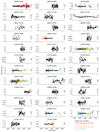 |
Fig. 1. Residuals from the timing model in Table 2 for all 35 pulsars. The different colours represent different instruments as indicated in the bottom-right corner. The black bars on the right side of each panel show the scale of the proportion of the spin period. |
Pulsar timing solutions.
Binary parameters for PSR J0828+5304.
2.3. Pulse profiles
The profiles at different frequencies were aligned by applying the model in Table 2 and then rotated such that the highest peak of the LOFAR pulse profile was located at a phase ϕ = 0.25. The averaged pulse profiles from the pulsars presented in this paper are shown in Fig. 2. Most pulse profiles were modelled with one, two, or three von Mises functions. Nearly all pulsars display a profile with a single main pulse, except for PSRs J0613+3731 and J0828+5304. The PSR J0613+3731 shows a very faint interpulse in the FR606 data, which is only just visible in the LOFAR Core data and is at a phase Δϕ = 0.4 from the main pulse. The binary pulsar J0828+5304 displays a clear interpulse at Δϕ = 0.5 of the main pulse.
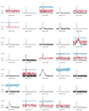 |
Fig. 2. Pulse profiles averaged over all observations of the pulsars at 149 MHz (black), 334 MHz (red), and 1532 MHz (blue) with bandwidths of 78, 64, and 384 MHz. The profiles were aligned by applying the model in Table 2. Then, all profiles were rotated such that the highest peak of the LOFAR pulse profile is located at phase ϕ = 0.25. The pulse profiles at 149 MHz have 1024 phase bins, while the profiles at 334 and 1532 MHz were rebinned from 512 and 1024 to 256 and 512 phase bins, respectively. |
We calculated full pulse widths at 10% (W10) and 50% (W50) of the peak intensity of the fully frequency- and time-averaged profiles at 149 MHz, 334 MHz, and 1484 or 1532 MHz, if available. Pulse widths were determined using tools from PSRSALSA (Weltevrede 2016), which models the profiles with analytical templates composed of one or more von Mises functions and calculates pulse widths from the added components. For the observations used for timing, we applied the templates that were created to calculate TOAs, while for all other observations, new templates were constructed. Uncertainties on the pulse widths were determined by generating a width distribution composed of simulated pulse profiles with randomly added noise from the off-pulse region of the added profiles and then calculating the standard deviation of the simulated width distribution. The pulse widths and duty cycles can be found in Table 4.
Pulse widths and duty cycles at 10% and 50% of the pulse amplitude at different frequencies.
2.4. Flux densities and spectral analysis
Mean flux densities were determined from the LOFAR Core, Lovell, and NRT observations. Observations from LOFAR were fully averaged in time and split into two sub-bands with centre frequencies of 129 and 166 MHz. For each pulsar, all observations at these frequencies were combined, and flux densities were calculated using the radiometer equation in the method used by Kondratiev et al. (2016). Combined with sky temperatures taken from Price (2021), this approach modelled the LOFAR beam, the system temperature, and the beamformer coherence. We found that, on average, between 5 and 10% of the dipoles in the LOFAR HBAs were not in operation, reducing the effective area (Kondratiev et al. 2016). We used a conservative estimate of 5% of broken antennas for all flux density calculations as to not overestimate the flux densities of the pulsars. For observations where 10% of the dipoles were not operational, the effect would be an underestimation of the flux density, which is much lower than the uncertainty from other factors. We assumed a systematic uncertainty due to RFI, scintillation, and fluctuating tied-array beam gain and system temperatures of 50%, as suggested in Kondratiev et al. (2016).
We note that we did not attempt to correct the LOFAR flux densities for positional offsets of the pulsars with respect to the centre of the LOFAR Core tied-array beam. Positional offsets are introduced by ionospheric effects, which can introduce random displacements of ∼1′ compared to the  full width half maximum (FWHM) of the tied-array beam during observations. More importantly, however, there are systematic offsets between the final timing position and the position determined from gridding and used to obtain the timing observations. For six pulsars, the gridding positions place them outside of the FWHM of the tied-array beam. While a squared sinc function was used to correct flux densities of known pulsars in Sanidas et al. (2019), this approach was not suitable in our case, as the FWHM of a tied-array beam from the LOFAR Core stations is smaller than that from the stations on the LOFAR Superterp by a factor of six. Hence, the LOFAR flux densities should be treated as indicative and should not be used for detailed studies. We expect that accurate flux densities of the LOTAAS pulsars will become available with the continued data releases from the LOFAR continuum imaging survey (Shimwell et al. 2017).
For PSRs J0059+6956, J0305+1123, J0813+2202, J0828+5304, J0935+3312, J1427+5211, J1953+3014, J1958+5650, and J2123+3624, the observing position was updated part way through the observing time span, resulting in smaller positional offsets for the later observations. Only the later observations with improved gridding position were used to determine flux densities for these pulsars.
From the Lovell observations, we obtained flux densities at 334 and 1532 MHz. For each pulsar, the observations were fully averaged in time and frequency and combined using PSRADD. Flux densities were calculated from the radiometer equation using a gain of 0.8 K Jy−1 for both centre frequencies. We applied an elevation-dependent system temperature to take into account spillover and sky temperatures from Price (2021). The NRT observations were calibrated using a noise diode that injected white noise into the receiver to allow for the transfer of the flux scale using observations of flux calibrators. To estimate the uncertainty of the flux density measurements σS in the Lovell and NRT observations, we applied a simplified version of the method used in Jankowski et al. (2018):  , with S as the measured flux density for each pulsar and N as the number of observations, which assumed a systematic uncertainty of 20% and a typical modulation index due to scintillation of 30%. In the case of non-detections in the Lovell and NRT observations, upper limits were determined by averaging all observations and calculating the 3σ limit of the root-mean-square (rms) noise of the pulse profile.
For the 29 pulsars whose timing positions fall within the FWHM of the LOFAR Core tied-array beam, we used Bayesian methods to model the radio spectra from both the flux density measurements and the upper limits. We used EMCEE (Foreman-Mackey et al. 2013) to maximise the likelihood function for detections and non-detections, as described by Laskar et al. (2014, Eqs. (1)–(3)). We assumed that the radio spectra could be modelled with a single power law, Sν = S0(ν/ν0)α, where Sν are the observed mean flux densities or upper limits at their respective observing frequencies ν and α as the spectral index for a flux density S0 at reference frequency ν0 = 149 MHz. Flat priors were assumed in S0 and for −9 < α < 3. We note that the simplification of a single power law may not be valid for all pulsars, as some pulsars may have spectra that are better described by a broken power law (e.g. Bilous et al. 2016; Jankowski et al. 2018).
3. Results
3.1. Timing
The timing residuals shown in Fig. 1 using the timing models from Tables 2 and 3 are generally noise-like (i.e. uncorrelated and around the same level as the TOA uncertainties) for the majority of pulsars. The residuals of PSRs J0139+5621, J0613+3731, and J2306+3124 display time-dependent trends, while the timing residuals of PSRs J0811+3729, J0928+3039, J1722+3519, and J1910+5655 show non-Gaussian noise, resulting in timing solutions with high reduced χ2 values.
In the case of PSR J0139+5621, the residuals of the LOFAR observations obtained after the observational gap between May 2018 and June 2019 show a downward trend, indicating the possibility of a glitch, a sudden increase in the spin frequency, which is often followed by a recovery towards the pre-glitch frequency (Radhakrishnan & Manchester 1969; Reichley & Downs 1969). By fitting the spin-frequency ν with the TOAs before and after MJD 58257 separately, we obtained a fractional glitch size Δν/ν of 3.3 × 10⁻¹⁰, which is near the lower values of the observed range of glitch sizes of 10−11 and 10−5 (Espinoza et al. 2011; Yu et al. 2013; Basu et al. 2022). As glitches are predominantly seen in younger pulsars and since PSR J0139+5621 is the youngest pulsar in our sample, with a characteristic age τc of 3.6 × 10⁵ yr (see the last paragraph of this section for further explanations on τc), we consider it likely that a glitch occurred in PSR J0139+5621.
We considered the possibility that the long-term trends seen in the residuals for PSRs J0613+3731 and J2306+3124 could be due to magnetic dipole braking. This would yield a measurable second spin-frequency derivative  for spin-frequency ν and spin-frequency derivative
  with n = 3. However, fitting for
  in the timing solutions of PSRs J0613+3731 and J2306+3124 yields unrealistically large values for |n|, indicating that the observed trends are likely due to timing noise, which is seen in the majority of normal pulsars timed over long time spans (e.g. Hobbs et al. 2010).
We found that the noise in the timing residuals of PSRs J0811+3729, J0928+3039, J1722+3519, and J1910+5655 is caused by nulling and pulse-to-pulse profile variations that do not average out over the length of the observation, see Fig. 3. We discuss some of these pulsars in Sect. 3.2.
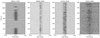 |
Fig. 3. Pulse profile variations with time for four pulsars at 149 MHz. The figures display multiple rotations per sub-integration. A portion of the full rotation is shown here, and the profiles have been rotated such that the highest peak is centred at phase ϕ = 0.25 or ϕ = 0.5. The flux scale was normalised for each pulsar separately. White bars indicate where RFI was removed from the data. |
For the majority of the pulsars, the offset between the timing position and the gridded position used to obtain the timing observations (Table 5) fall within the  half width at half maximum (HWHM) of the tied-array beams with the LOFAR Core. For PSR J0305+1123, the position used to obtain the observations was updated in November 2017, resulting in higher signal-to-noise detections and more precise TOAs (Fig. 1). Of the six outliers (PSRs J0317+1328, J1814+2224, J1958+2214, J2006+2205, J2057+2128, and J2306+3124), nearly all have offsets below
  . The only exception is PSR J1958+2214, which is offset by
  and located in the far side lobes of the LOFAR Core tied-array beam. The origin of this large offset was traced back to the LOTAAS survey observation in which PSR J1958+2214 was discovered, which showed several high signal-to-noise detections at widely separated tied-array beams. These odd side lobe detections were noted at the time of observation, and the choice was made to perform follow-up gridding observations using more narrow tied-array beams towards the detections of two neighbouring tied-array beams in the centre of the hexagonal grid of 61 LOFAR Superterp tied-array beams. Ultimately, the actual position of PSR J1958+2214 turned out to be consistent with one of the detections in the outer ring of the hexagonal grid.
Significant measurements of proper motion were obtained for PSRs J0828+5304 and J2053+1718. The proper motion of PSR J0828+5304 is μα cos δ = 4.8 ± 1.8 mas yr−1 and μδ = −14 ± 3 mas yr−1, yielding transverse velocities of 63 and 110 km s−1 for the 0.9 and 1.6 kpc distances predicted by the NE2001 (Cordes & Lazio 2002) and YMW16 (Yao et al. 2017) Galactic electron density models. For PSR J2053+1718, with μα cos δ = −31 ± 5 mas yr−1 and μδ = 15 ± 9 mas yr−1, the transverse velocities are 315 and 344 km s−1 at the NE2001 distance of 1.9 kpc and the YMW16 distance of 2.1 kpc. The pulsar PSR J2053+1718 was first discovered by Arecibo (Ray et al. 1996), and a timing solution for the pulsar has recently been published by Brinkman et al. (2018). They obtained significantly lower transverse velocities of 63 and 69 km s−1 for the NE2001 and YMW16 distances over a longer timing baseline. As Brinkman et al. (2018) reports DM variations on the order of 5 × 10⁻³ pc cm−3, we attribute the larger LOTAAS proper motion measurement, as well as the high reduced χ2 of the LOTAAS timing solution, to unmodelled DM variations affecting the arrival time measurements. Based on the short spin period and low magnetic field, Brinkman et al. (2018) propose that PSR J2053+1718 may be a disrupted recycled pulsar, that is a pulsar which was spun up in a binary system with a massive stellar companion that became disrupted and unbound when the companion went supernova. This origin could explain the low magnetic field of the system, which is typically seen in double neutron star systems (DNSs; see Tauris et al. 2017 for a review on DNSs).
The period and period derivative from the timing models were used to calculate the characteristic age τc, the surface magnetic field strength B, and the intrinsic spin-down energy Ė (see the rightmost columns in Table 5). For obtaining these estimates, we assumed a canonical neutron star with a radius of 10 km and a moment of inertia of 1045 g cm2. Furthermore, we assumed that the initial spin is negligible and that magnetic dipole radiation is responsible for the spin-down throughout the pulsar’s lifetime (see Lorimer & Kramer 2012 for details).
3.2. Pulse profile variations
The pulse profiles of some of the LOTAAS pulsars show profile variations in time or frequency. Figures 3 and 4 highlight these variations.
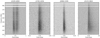 |
Fig. 4. Pulse profile variations with frequency of four pulsars between the frequencies 110 and 188 MHz. A portion of the full rotation is shown here, and the profiles have been rotated such that the highest peak is centred at phase ϕ = 0.25 or ϕ = 0.5. The flux scale was normalised for each pulsar separately. White bars indicate where RFI was removed from the data. |
The pulsar PSR J0811+3729 is the most extreme case due to its display of nulling, a relatively common phenomenon where the pulsed emission temporarily ceases. In other pulsars, nulls have been observed to last between a single pulsar rotation up to several weeks (e.g. Kramer et al. 2006; Young et al. 2015; Basu et al. 2017). In the absence of observations with single pulse integrations, we analysed the energy distributions of the 5-s sub-integrations where each sub-integration covers just over four individual pulses. For each sub-integration, we determined whether pulsed emission was present by applying the criteria from Wang et al. (2020), which compare the emission in the on-pulse region with the standard deviation of the emission in the off-pulse region. We found that for the total observation length of PSR J0811+3729 of 14.4 h, 80.1% of 5-s sub-integrations were in a null state. The mean length of a null state was 105 s, with the longest null lasting a full observation period of 20 min. The average time between nulls was approximately 29 s, and the longest time the pulsar was in an emission state was 5.67 min.
For PSR J0928+3039, the 5-s sub-integrations covered 3.43 individual pulses and, as shown in a representative observation in Fig. 3, these revealed strong variability on timescales of tens of seconds. The strong variations appear to occur primarily in the leading half of the profile. Pulsed emission was also absent for occasional sub-integrations, indicating that this pulsar may be nulling for a few rotations at a time. No evidence for drifting sub-pulses was visible, but completely ruling out the possiblity would require observations of individual pulses.
The profile of PSR J1722+3519 at 149 MHz shows two narrow components whose amplitude varies between observations, resulting in the additional noise seen in the timing residuals. In most observations, the leading component of the averaged pulse profile has half the amplitude of the trailing component, but in some observations, both components have comparable amplitudes. The 5-s sub-integrations (6.08 individual pulses) reveal that these variations in the averaged profiles are caused by pulse-to-pulse variations between the individual pulse components. To understand the profile variability of PSR J1722+3519, a one-hour observation where individual pulses were recorded was obtained and analysed. This observation revealed a highly variable intensity of the two profile peaks with a relatively long timescale of ∼100 pulse periods. A fluctuation spectrum analysis using the methods described in Weltevrede (2016) confirmed the presence of this modulation timescale. For many pulsars, periodic intensity modulation can be associated with drifting sub-pulses (e.g. Song et al. 2022). However, for PSR J1722+3519, only evidence for amplitude modulation is found. Given the long timescale of the modulation, even longer observations would be beneficial to revealing any associated phase variations. Another possible explanation for the profile variation and the large rms residuals is short timescale mode switching, as seen in Stairs et al. (2019) for example.
In the case of PSR J1910+5655, 14.63 individual pulses were averaged into the 5-s sub-integrations, which still show significant variability between sub-integrations. The relatively low signal-to-noise of the profile in the 5-s sub-integrations combined with the averaging of many pulses per sub-integration and the single wide component (21% duty cycle) make it difficult to classify these variations.
The pulse profile of PSR J1529+4050 displays multiple components at 149 MHz, and in the LOFAR band between 110 and 188 MHz, the leading component decreases in brightness with increasing frequency compared to the trailing component (Fig. 4). At 334 MHz and 1532 MHz, only the trailing component remains (Fig. 2), indicating that the leading component has significantly steeper spectra compared to the trailing component. In a study comparing the pulse profiles of a hundred pulsars observed by the LOFAR HBAs as well as the Lovell telescope at L-band, Pilia et al. (2016) found pulse profiles with more profile components at HBA frequencies compared to L-band frequencies to be less common than the other way around. More components at HBA frequencies may be explained by the presence of a wider pulsar beam at lower frequencies (Cordes 1978), resulting in more components coming into view. Pilia et al. (2016) note a slight indication that pulsars with more components at HBA frequencies than at L-band frequencies may be older and have a longer period. With a characteristic age of 2.8 × 10⁹ yr, PSR J1529+4050 is the fourth oldest pulsar in our sample.
3.3. Pulse widths
Figure 5 shows the pulse widths at 50% of the peak profile intensity of all LOTAAS discoveries, combining the W50 values from this paper with those reported in Michilli et al. (2020), Tan et al. (2018, 2020). Because the W50 of PSRs J0250+5854 and J1658+3630 were reported at slightly different observing frequencies, we used the W50 value at a frequency nearest to the frequencies used in this section. We found that, on average, the pulse widths are somewhat wider at 149 MHz than at the higher frequencies, with a mean W50 at 149 MHz of 29 ms and a standard deviation of 33 ms, compared to 24 ± 20 ms and 27 ± 28 ms at 334 and 1532 MHz, respectively.
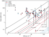 |
Fig. 5. The relations between pulse broadening and DM as found by Bhat et al. (2004; dashed lines) and Geyer et al. (2017; solid lines) at 149, 334, and 1532 MHz in black, red, and blue, respectively. The functions from Geyer et al. (2017) are shown with scattering indices between −4 and −2, while the function from Bhat et al. (2004) is displayed with the best fitting index of −3.68. Shown as dots, circles, and squares are the W50 pulse widths from this study, as well as from the previous LOTAAS reports of Tan et al. (2018, 2020), Michilli et al. (2020) at different frequencies. These measurements represent upper limits on pulse broadening due to interstellar scattering. Pulse widths from the same pulsar at different frequencies are connected with grey vertical lines. The pulsars discussed in Sect. 3.3 are marked with arrows. The pulse widths of eight pulsars at 149 MHz from Michilli et al. (2020) and Tan et al. (2020), which may be affected by scattering, are marked with grey circles. |
The intrinsic profile of pulsars becomes broadened by the effects of interstellar scattering, resulting in exponential tails at the trailing edge of the pulse profiles. Four pulsars from the sample reported here, PSRs J1745+4254, J2006+2205, J2123+3624, and J2306+3124, show these effects in the pulse profiles at 149, 334, and/or 1484 or 1532 MHz (see Figs. 2 and 4), suggesting that they may be scatter broadened. These pulsars are shown in Fig. 5, as are eight pulsars that Michilli et al. (2020) and Tan et al. (2020) reported as showing signs of scatter broadening. All of these pulsars are at DMs above 20 pc cm−3, which is expected since scatter broadening is caused by material in the interstellar medium and is hence roughly correlated with the DM.
Figure 5 also displays the scatter broadening predictions at 149, 334, and 1532 MHz from the empirical relations between scattering and DM found by Bhat et al. (2004) and Geyer et al. (2017). Most pulse widths displayed in Fig. 5 are around the same order of magnitude as the scatter broadening predicted by Bhat et al. (2004) and Geyer et al. (2017) for the typical scattering indices of αS ∼ −4 or −4.4 (for scattering timescales τν ∝ ναS) from the thin screen approximation (Williamson 1972). Hence, the scattering relations predict that the pulse profiles of the majority of the pulsars in our sample should be affected by interstellar scattering. However, most pulse profiles in Fig. 2, as well as the pulse profiles from the previous LOTAAS timing papers, do not show signs of scattering, suggesting that there is a less steep frequency scaling (αS > −4) or that the scattering timescales may be smaller than predicted by Bhat et al. (2004) and Geyer et al. (2017).
To test this, we modelled the frequency dependence of the LOFAR pulse profiles of the pulsars that show exponentially trailing edges, PSRs J1745+4254, J2006+2205, J2123+3624, and J2306+3124, with the wideband pulsar timing code PULSEPORTRAITURE by Pennucci (2019), which simultaneously measures TOAs, DM, and scattering by fitting frequency dependent templates. With this method, we constrained a scattering time τS and scattering index αS for these four pulsars by modelling the intrinsic profile as a single Gaussian function and the pulse broadening as a one-sided exponential function. We fitted this model to an averaged pulse profile combining all LOFAR observations, which were fully averaged in time and partially averaged in frequency to 100 frequency channels.
We found that the LOFAR profile of PSR J1745+4254 is best modelled with a large scattering index of αS = −1.10 ± 0.12 and a scattering timescale of τS = 5.49 ± 8 ms. Similarly, PSR J2006+2205 has a large scattering index of αS = −2.18 ± 15 for τS = 15.8 ± 3 ms, while PSR J2123+3624 has a more typical scattering index of αS = −3.55 ± 9 for τS = 89.6 ± 1.0 ms. We note that the profile of PSR J2306+3124 displays a similar exponential tail at both 149 MHz and 1532 MHz, with no discernible frequency evolution between the observing bands, indicating its intrinsic profile may have an exponential tail. The large scattering indices of PSRs J1745+4254 and J2006+2205 confirm that the effect of scatter broadening in the LOFAR pulse profiles is less pronounced compared to predictions from the typical −4 and −4.4 scattering index values, behaviour also reported in other pulsars at low observing frequencies (Geyer et al. 2017).
3.4. Spectral index
Table 5 displays the flux densities and the spectral indices, and Fig. 6 shows the mean flux densities and the spectral power laws. For the 29 pulsars investigated, we obtained a mean spectral index of α = −2.8 ± 1.5, with the uncertainty representing the standard deviation, which is consistent with the values of α = −2.4 ± 0.9 and α = −1.9 ± 0.5 from Michilli et al. (2020) and Tan et al. (2020), respectively, despite slightly different treatments of the flux calibration and spectral fitting. Of the pulsars with spectral index measurements, PSR J2336−0152 displays a notably steep spectrum with a spectral index of −5 ± 2 due to the large difference between the measured flux densities at 129 and 166 MHz. However, these flux densities have large uncertainties and a much flatter spectrum is also consistent with our results. We highlight that a simple power law may be insufficient to describe the spectra of some pulsars.
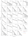 |
Fig. 6. Mean flux densities (dots and circles) and upper limits for flux densities (triangles) as reported in Table 5 for the 29 pulsars whose timing positions fall within the FWHM of the LOFAR Core tied-array beam. Filled dots and triangles are flux density measurements for which five or more observations were available, while empty circles and triangles are measurements from less than five observations. The black lines represent fitted spectral indices, which are the mean values for the spectral index α and the flux density on the reference frequency of 149 MHz S0 from the EMCEE samples. The shaded regions represent the uncertainty on α and S0 propagated to flux densities between 90 and 2100 MHz. For the spectral index fit, only flux density measurements with five or more observations were used. |
3.5. PSR J0828+5304
PSR J0828+5304 is a binary millisecond pulsar with a spin period of 13.52 ms at a DM of 23.103 pc cm−3. Table 3 provides the binary parameters of this pulsar. The orbital period of Pb = 5.899 d and the projected semi-major axis of x = 13.147 lt-s yield a mass function of 0.07 M⊙, constraining the binary companion mass to 0.65 M⊙ for an edge-on orbit, or 0.79 M⊙ for a median orbital inclination of 60°, assuming the pulsar has a canonical mass of 1.4 M⊙. With this companion mass and spin period, PSR J0828+5304 can be classified as an intermediate-mass binary pulsar (van Kerkwijk et al. 2005) where the neutron star is partially recycled due to unstable mass transfer from a binary companion that will leave a CO or ONeMg-core white dwarf (Tauris et al. 2012). The Laplace-Lagrange parameters of the ELL1 binary model for nearly circular orbits yield an orbital eccentricity of 2.5(7)×10−6, in line with predictions from tidal orbital circularisation (Phinney 1992; Phinney & Kulkarni 1994).
No optical counterpart is present at the pulsar timing position of PSR J0828+5304 in the Pan-STARSS1 survey (PS1; Chambers et al. 2016); the nearest catalogued PS1 source is 24″ offset. The nominal PS1 5σ detection limit of r-band magnitude r = 23.2 provides absolute magnitude limits of Mr > 12.2 for the 0.9 and 1.6 kpc distances estimated from the observed DM and the NE2001 (Cordes & Lazio 2002) and YMW16 (Yao et al. 2017) Galactic electron density models, respectively. At this limit, cooling models3 by Bergeron et al. (2011) and Tremblay et al. (2011) for 0.7 M⊙ white dwarfs with either hydrogen or helium atmospheres predict effective temperatures and white dwarf cooling ages of Teff < 12 000 K and τcool > 0.5 Gyr, ruling out young and hot white dwarf companions.
4. Discussion and conclusions
We presented the properties of 35 pulsars discovered with LOFAR as part of the LOTAAS (Sanidas et al. 2019) and LOFAR pilot surveys (Coenen et al. 2014). We expanded this sample with the properties of 41 LOFAR-discovered pulsars reported by Michilli et al. (2020), Tan et al. (2018, 2020), all of which were discovered by the LOTAAS survey. We excluded PSR J0815+4611, whose timing parameters were presented in Michilli et al. (2020), as it was discovered as a steep spectrum polarised point source in continuum images of the 3C 196 field (Jelić et al. 2015). Similarly, we excluded radio pulsars discovered with LOFAR and presented by Pleunis et al. (2017), Bassa et al. (2017, 2018), and Sobey et al. (2022), as these pulsars were discovered through the use of coherent dedispersion and by targeting the locations of Fermiγ-ray sources or polarised point sources from the LOFAR imaging survey (Shimwell et al. 2017) and will have different survey selection effects compared to LOTAAS.
The spectral properties of the LOTAAS sample have a mean spectral index, assuming power law spectra of the form Sν ∝ να, of α = −2.5 with a standard deviation of 1.2 (for 66 pulsars), see Fig. 7. On average, these spectra are steeper compared to the sample studied by Jankowski et al. (2018), which has α = −1.57 ± 0.62 for 441 radio pulsars at radio frequencies between 728 and 3100 MHz. They are also steeper than the single power law spectral fits by Bilous et al. (2016), which have α = −1.4 ± 0.7 for 124 pulsars, with observations from the LOFAR band between 110 and 188 MHz, the same band used for the LOTAAS timing observations presented in this paper.
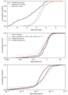 |
Fig. 7. Cumulative distributions of the spectral index, the spin period, and the period derivative of the pulsars discovered by the LOTAAS survey (black). The upper plot displays spectral indices from Jankowski et al. (2018; blue) and Bilous et al. (2016; orange). We emphasise that due to the uncertainties in the flux calibration of the LOTAAS obervations, the LOTAAS spectral indices should not be used for detailed studies. The lower plots show the LOTAAS redetections (red), the known pulsar population (grey), and a subset of the known pulsar population limited to P > 0.02 s and DM < 200 pc cm−3 (blue). |
The steeper radio spectra of LOTAAS-discovered pulsars are readily explained as a selection effect, as pulsars with flatter spectra will already have been discovered by earlier pulsar surveys at higher frequencies. In particular, the LOTAAS survey overlaps with the GBNCC survey of the northern sky using the Green Bank telescope (Stovall et al. 2014), which started in 2009 and reaches a sensitivity of 1.1 mJy at 350 MHz; the AO327 survey with Arecibo, reaching 0.4 mJy at 327 MHz for declinations between −1° and 28° and which started survey observations in 2011 (Deneva et al. 2013); and PUMPS with the Large Phased Array at Pushchino, which started in 2014, with sensitivities up to 0.1 mJy at 111 MHz for declinations between −9° and 42° (Tyul’bashev et al. 2022). Of the 311 known radio pulsars redetected with LOTAAS, 47 were earlier discoveries from the GBNCC survey and six were from the AO327 survey (Sanidas et al. 2019), indicating that these pulsars would have been new discoveries for LOTAAS in the absence of the GBNCC and AO327 surveys. Similarly, the pulsars discovered with LOTAAS and detected at 334 MHz with the Lovell telescope have 334 MHz flux densities near the sensitivity limits of the GBNCC and AO327 surveys, indicating the LOTAAS-discovered pulsars were likely below the detection thresholds of the GBNCC and AO327 surveys.
The timing solutions of the LOTAAS pulsars show that they have, on average, longer spin periods and lower spin period derivatives in comparison to the known population of radio pulsars. These findings confirm the results from Sanidas et al. (2019), who already noted the LOTAAS-discoverd spin periods as being longer than those from the known population. To compare the LOTAAS spin periods and spin period derivatives with those of the known pulsar population, we constructed three pulsar samples: (I) the LOTAAS discoveries; (II) known pulsars that were redetected in the LOTAAS survey, and (III) known radio pulsars that were not detected in LOTAAS and that have P > 0.02 s and DM < 200 pc cm−3, to take into account some of the selection biases of LOTAAS, namely the increased sensitivity towards slower pulsars and decreased sensitivity for pulsars at high DM (Sanidas et al. 2019). We queried the ATNF pulsar catalogue4 (version 1.67, Manchester et al. 2005) for the properties of the known pulsars in order to construct samples II and III, where we excluded pulsars that were associated with globular clusters. For sample II, the redetected pulsars presented in Sanidas et al. (2019), spin period, and spin period derivatives were available for 253 out of the 311 pulsars, while sample III consists of 891 pulsars.
Figure 7 shows the cumulative distributions of the spin period and spin period derivatives of the three samples, as well as the entire known pulsar population. Using two-sample Kolmogorov–Smirnov (KS) tests, we found that the probability that the spin periods and spin period derivatives of sample I, the LOTAAS discoveries, are drawn from the selection-bias-corrected known pulsar population (sample III) is low, at p = 0.73% and 0.039%, respectively. As these probabilities are p < 1%, we can reject the null hypothesis that the samples were drawn from the same underlying distribution. For comparison, the probability that the known pulsars redetected by LOTAAS, sample II, are drawn from sample III is significantly higher, p = 33% for the spin period distribution and 30% for the spin period derivative distribution.
Assuming that the spin period P and spin period derivative Ṗ distributions from Fig. 7 both follow a log-normal distribution, we found log10P = −0.040 ± 0.421 and log10 Ṗ = −15.43 ± 1.10 for the median spin period (P in s) and spin period derivatives (Ṗ in s s−1) of the LOTAAS discoveries (sample I), compared to log10P = −0.20 ± 0.43 and log10 Ṗ = −14.94 ± 1.18 for the known pulsar population with P > 0.02 s and DM < 200 pc cm−3 (sample III). Hence, the LOTAAS-discovered pulsars have spin periods and spin-down rates that are, on average, a factor 1.4 longer and a factor 3.1 lower, respectively, compared to the known pulsar population.
When plotted in a P − Ṗ-diagram, Fig. 8, the LOTAAS discoveries have higher characteristic ages τc and lower spin-down luminosities Ė and are generally located closer to the pulsar deathlines where pulsar emission ceases (e.g. Chen & Ruderman 1993; Zhang et al. 2000). The cause of these offsets in spin period and spin period derivative is not immediately obvious, though Sanidas et al. (2019) remarked that the 3600 s integration times of LOTAAS, which is significantly longer than those of many other pulsar surveys, will increase its sensitivity towards longer period pulsars.
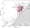 |
Fig. 8. P − Ṗ diagram of the pulsars discovered (black dots) and redetected (red circles) by the LOTAAS survey and the known pulsar population (grey dots). The grey dotted and dashed diagonals represent the characteristic ages and the spin-down luminosities, respectively. The solid lines are deathlines from Chen & Ruderman (1993) and Zhang et al. (2000). |
The offsets may also be related to the low observing frequency of the LOTAAS survey compared to previous surveys, making LOTAAS more sensitive to pulsars with steeper radio spectra. Jankowski et al. (2018) found strong correlations of the spectral index α with the spin-down luminosity Ė, magnetic field at the light cylinder BLC, the spin frequency derivative  , and the characteristic age τc. They found the maximum Spearman correlation coefficient between α values of 276 pulsars and a parameterisation of their spin frequency ν and
  in the form of
  for values that have b/a = 0.55. Converting this parameterisation from ν and
  to P and Ṗ using
  , we found that the b/a = 0.55 correlation corresponds to r/q = −0.26 (as r/q = ( − a/b − 2)−1). This indicates that for 1 dex in P, Ṗ decreases by 0.26 dex in the P − Ṗ diagram of Fig. 8 and that pulsars with steeper radio spectra generally have longer spin periods and lower spin period derivatives.
Longer spin periods and lower spin period derivatives are also seen for pulsars recently discovered with the GBNCC survey (Lynch et al. 2018), as well as those from the SUPERB survey (Spiewak et al. 2020) with Parkes. While the GBNCC survey observing at 350 MHz will also be biased towards pulsars with steeper radio spectra, the SUPERB survey, observing at 1382 MHz (Keane et al. 2018) will not, as the majority of pulsars making up the known pulsar population were discovered at those observing frequencies (Edwards et al. 2001; Manchester et al. 2001; Cordes et al. 2006; Keith et al. 2010). For the GBNCC survey, population synthesis modelling by McEwen et al. (2020) revealed that this bias is introduced through the GBNCC’s reduced sensitivity towards pulsars at low Galactic latitudes, due to increased sky temperatures and scattering and the fact that young radio pulsars have not had enough time to move away from their birthplaces in the Galactic plane (Faucher-Giguère & Kaspi 2006). Hence, the GBNCC survey is biased towards finding pulsars at higher Galactic latitudes, which are predominantly older pulsars. This is also the case for the SUPERB survey discoveries, as it specifically targets higher Galactic latitudes (|b|> 15°; Keane et al. 2018), as well as LOTAAS, which has worse sensitivity in the Galactic plane compared to the GBNCC survey due to increased sky temperatures and the effects of scattering.
We consider it likely that all three effects combined (i.e. sensitivity to longer spin periods, steeper radio spectra, and the reduced sensitivity towards young pulsars in the Galactic plane) play a role in discovering pulsars with longer spin periods and lower spin-down rates. However, we cannot rule out that older pulsars have, on average, steeper radio spectra. Pulsar population synthesis modelling would be required to estimate the impact of each of these effects separately and separate those from any intrinsic pulsar properties, such as a correlation between age and the steepness of the pulsars radio spectra. This task goes beyond the scope of this paper, as these simulations would benefit from using new and updated models of the Galactic electron distribution, the global sky temperature, and scattering (e.g. Yao et al. 2017; Price 2021; Geyer et al. 2017) to properly model the sensitivity for the low observing frequencies of the LOTAAS survey.
Advanced Radio Transient Event Monitor and Identification System.
http://www.astro.umontreal.ca/ergeron/CoolingModels
Acknowledgments
The paper is based (in part) on data obtained with the International LOFAR Telescope (ILT) under project codes LC1_003, LT3_001, LC4_004, LT5_003, LT5_004, LC9_021, LC9_041, LT10_015 and LT14_005. LOFAR (van Haarlem et al. 2013) is the Low Frequency Array designed and constructed by ASTRON. It has observing, data processing, and data storage facilities in several countries, that are owned by various parties (each with their own funding sources), and that are collectively operated by the ILT foundation under a joint scientific policy. The ILT resources have benefitted from the following recent major funding sources: CNRS-INSU, Observatoire de Paris and Université d’Orléans, France; BMBF, MIWF-NRW, MPG, Germany; Science Foundation Ireland (SFI), Department of Business, Enterprise and Innovation (DBEI), Ireland; NWO, The Netherlands; The Science and Technology Facilities Council, UK. We acknowledge the use of the Nançay Data Center computing facility (CDN – Centre de Données de Nançay). The CDN is hosted by the Nançay Radioastronomy Observatory (ORN) in partnership with Observatoire de Paris, Université d’Orléans, OSUC and the CNRS. The CDN is supported by the Région Centre-Val de Loire, département du Cher. The Nançay Radio Observatory is operated by the Paris Observatory, associated with the French Centre National de la Recherche Scientifique (CNRS). This research was made possible by support from the Dutch National Science Agenda, NWA Startimpuls – 400.17.608. C.G.B., J.W.T.H., V.I.K., and D.M. acknowledge support for this work from the European Research Council under the European Union’s Seventh Framework Programme (FP/2007-2013)/ERC Grant Agreement nr. 337062.
References
- Bassa, C. G., Pleunis, Z., Hessels, J. W. T., et al. 2017, ApJ, 846, L20 [NASA ADS] [CrossRef] [Google Scholar]
- Bassa, C. G., Pleunis, Z., Hessels, J. W. T., et al. 2018, in Pulsar Astrophysics the Next Fifty Years, eds. P. Weltevrede, B. B. P. Perera, L. L. Preston, & S. Sanidas, 337, 33 [NASA ADS] [Google Scholar]
- Basu, R., Mitra, D., & Melikidze, G. I. 2017, ApJ, 846, 109 [NASA ADS] [CrossRef] [Google Scholar]
- Basu, A., Shaw, B., Antonopoulou, D., et al. 2022, MNRAS, 510, 4049 [NASA ADS] [CrossRef] [Google Scholar]
- Bergeron, P., Wesemael, F., Dufour, P., et al. 2011, ApJ, 737, 28 [Google Scholar]
- Bhat, N. D. R., Cordes, J. M., Camilo, F., Nice, D. J., & Lorimer, D. R. 2004, ApJ, 605, 759 [CrossRef] [Google Scholar]
- Bhattacharyya, B., Cooper, S., Malenta, M., et al. 2016, ApJ, 817, 130 [NASA ADS] [CrossRef] [Google Scholar]
- Bilous, A. V., Kondratiev, V. I., Kramer, M., et al. 2016, A&A, 591, A134 [NASA ADS] [CrossRef] [EDP Sciences] [Google Scholar]
- Brinkman, C., Freire, P. C. C., Rankin, J., & Stovall, K. 2018, MNRAS, 474, 2012 [NASA ADS] [CrossRef] [Google Scholar]
- Broekema, P. C., Mol, J. J. D., Nijboer, R., et al. 2018, Astron. Comput., 23, 180 [NASA ADS] [CrossRef] [Google Scholar]
- Burgay, M., D’Amico, N., Possenti, A., et al. 2003, Nature, 426, 531 [NASA ADS] [CrossRef] [Google Scholar]
- Caleb, M., Heywood, I., Rajwade, K., et al. 2022, Nat. Astron., 6, 1 [Google Scholar]
- Chambers, K. C., Magnier, E. A., Metcalfe, N., et al. 2016, ArXiv e-prints [arXiv:1612.05560] [Google Scholar]
- Chen, K., & Ruderman, M. 1993, ApJ, 402, 264 [NASA ADS] [CrossRef] [Google Scholar]
- Coenen, T., van Leeuwen, J., Hessels, J. W. T., et al. 2014, A&A, 570, A60 [NASA ADS] [CrossRef] [EDP Sciences] [Google Scholar]
- Cordes, J. M. 1978, ApJ, 222, 1006 [NASA ADS] [CrossRef] [Google Scholar]
- Cordes, J. M., & Lazio, T. J. W. 2002, ArXiv e-prints [arXiv:astro-ph/0207156] [Google Scholar]
- Cordes, J. M., Freire, P. C. C., Lorimer, D. R., et al. 2006, ApJ, 637, 446 [NASA ADS] [CrossRef] [Google Scholar]
- Deneva, J. S., Stovall, K., McLaughlin, M. A., et al. 2013, ApJ, 775, 51 [NASA ADS] [CrossRef] [Google Scholar]
- Donner, J. Y., Verbiest, J. P. W., Tiburzi, C., et al. 2020, A&A, 644, A153 [EDP Sciences] [Google Scholar]
- Edwards, R. T., Bailes, M., van Straten, W., & Britton, M. C. 2001, MNRAS, 326, 358 [NASA ADS] [CrossRef] [Google Scholar]
- Espinoza, C. M., Lyne, A. G., Stappers, B. W., & Kramer, M. 2011, MNRAS, 414, 1679 [NASA ADS] [CrossRef] [Google Scholar]
- Faucher-Giguère, C.-A., & Kaspi, V. M. 2006, ApJ, 643, 332 [CrossRef] [Google Scholar]
- Folkner, W. M., & Park, R. S. 2016, JPL Planetary and Lunar Ephemeris DE436, https://naif.jpl.nasa.gov/pub/naif/JUNO/kernels/spk/de436s.bsp.lbl [Google Scholar]
- Foreman-Mackey, D., Hogg, D. W., Lang, D., & Goodman, J. 2013, PASP, 125, 306 [Google Scholar]
- Geyer, M., Karastergiou, A., Kondratiev, V. I., et al. 2017, MNRAS, 470, 2659 [NASA ADS] [CrossRef] [Google Scholar]
- Guillemot, L., Smith, D. A., Laffon, H., et al. 2016, A&A, 587, A109 [NASA ADS] [CrossRef] [EDP Sciences] [Google Scholar]
- Hewish, A., Bell, S. J., Pilkington, J. D. H., Scott, P. F., & Collins, R. A. 1968, Nature, 217, 709 [NASA ADS] [CrossRef] [Google Scholar]
- Hobbs, G. B., Edwards, R. T., & Manchester, R. N. 2006, MNRAS, 369, 655 [Google Scholar]
- Hobbs, G., Lyne, A. G., & Kramer, M. 2010, MNRAS, 402, 1027 [NASA ADS] [CrossRef] [Google Scholar]
- Hotan, A. W., van Straten, W., & Manchester, R. N. 2004, PASA, 21, 302 [Google Scholar]
- Hurley-Walker, N., Zhang, X., Bahramian, A., et al. 2022, Nature, 601, 526 [NASA ADS] [CrossRef] [Google Scholar]
- Jankowski, F., van Straten, W., Keane, E. F., et al. 2018, MNRAS, 473, 4436 [Google Scholar]
- Jelić, V., de Bruyn, A. G., Pandey, V. N., et al. 2015, A&A, 583, A137 [Google Scholar]
- Karastergiou, A., Chennamangalam, J., Armour, W., et al. 2015, MNRAS, 452, 1254 [NASA ADS] [CrossRef] [Google Scholar]
- Keane, E., Bhattacharyya, B., Kramer, M., et al. 2015, Advancing Astrophysics with the Square Kilometre Array (AASKA14), 40 [Google Scholar]
- Keane, E. F., Barr, E. D., Jameson, A., et al. 2018, MNRAS, 473, 116 [NASA ADS] [CrossRef] [Google Scholar]
- Keith, M. J., Jameson, A., van Straten, W., et al. 2010, MNRAS, 409, 619 [Google Scholar]
- Kondratiev, V. I., Verbiest, J. P. W., Hessels, J. W. T., et al. 2016, A&A, 585, A128 [NASA ADS] [CrossRef] [EDP Sciences] [Google Scholar]
- Kramer, M., Lyne, A. G., O’Brien, J. T., Jordan, C. A., & Lorimer, D. R. 2006, Science, 312, 549 [NASA ADS] [CrossRef] [Google Scholar]
- Kramer, M., Stairs, I. H., Manchester, R. N., et al. 2021, Phys. Rev. X, 11, 041050 [NASA ADS] [Google Scholar]
- Lange, C., Camilo, F., Wex, N., et al. 2001, MNRAS, 326, 274 [NASA ADS] [CrossRef] [Google Scholar]
- Laskar, T., Berger, E., Tanvir, N., et al. 2014, ApJ, 781, 1 [Google Scholar]
- Lazarus, P., Brazier, A., Hessels, J. W. T., et al. 2015, ApJ, 812, 81 [NASA ADS] [CrossRef] [Google Scholar]
- Lazarus, P., Karuppusamy, R., Graikou, E., et al. 2016, MNRAS, 458, 868 [Google Scholar]
- Lorimer, D. R., & Kramer, M. 2012, Handbook of Pulsar Astronomy (Cambridge: Cambridge University Press, UK) [Google Scholar]
- Lynch, R. S., Swiggum, J. K., Kondratiev, V. I., et al. 2018, ApJ, 859, 93 [NASA ADS] [CrossRef] [Google Scholar]
- Lyne, A. G., Burgay, M., Kramer, M., et al. 2004, Science, 303, 1153 [CrossRef] [PubMed] [Google Scholar]
- Manchester, R. N., Lyne, A. G., Camilo, F., et al. 2001, MNRAS, 328, 17 [NASA ADS] [CrossRef] [Google Scholar]
- Manchester, R. N., Hobbs, G. B., Teoh, A., & Hobbs, M. 2005, VizieR Online Data Catalog: VII/245 [Google Scholar]
- McEwen, A. E., Spiewak, R., Swiggum, J. K., et al. 2020, ApJ, 892, 76 [NASA ADS] [CrossRef] [Google Scholar]
- McLaughlin, M. A., Lyne, A. G., Lorimer, D. R., et al. 2006, Nature, 439, 817 [NASA ADS] [CrossRef] [Google Scholar]
- Michilli, D., Bassa, C., Cooper, S., et al. 2020, MNRAS, 491, 725 [Google Scholar]
- Morello, V., Barr, E. D., Cooper, S., et al. 2019, MNRAS, 483, 3673 [NASA ADS] [CrossRef] [Google Scholar]
- Pennucci, T. T. 2019, ApJ, 871, 34 [NASA ADS] [CrossRef] [Google Scholar]
- Petit, G. 2010, Highlights Astron., 15, 220 [NASA ADS] [Google Scholar]
- Phinney, E. S. 1992, Philos. Trans. R. Soc. London Ser. A, 341, 39 [NASA ADS] [CrossRef] [Google Scholar]
- Phinney, E. S., & Kulkarni, S. R. 1994, ARA&A, 32, 591 [NASA ADS] [CrossRef] [Google Scholar]
- Pilia, M., Hessels, J. W. T., Stappers, B. W., et al. 2016, A&A, 586, A92 [NASA ADS] [CrossRef] [EDP Sciences] [Google Scholar]
- Pleunis, Z., Bassa, C. G., Hessels, J. W. T., et al. 2017, ApJ, 846, L19 [Google Scholar]
- Price, D. C. 2021, Res. Notes Am. Astron. Soc., 5, 246 [Google Scholar]
- Radhakrishnan, V., & Manchester, R. N. 1969, Nature, 222, 228 [NASA ADS] [CrossRef] [Google Scholar]
- Ray, P. S., Thorsett, S. E., Jenet, F. A., et al. 1996, ApJ, 470, 1103 [NASA ADS] [CrossRef] [Google Scholar]
- Reichley, P. E., & Downs, G. S. 1969, Nature, 222, 229 [NASA ADS] [CrossRef] [Google Scholar]
- Romani, R. W., Kandel, D., Filippenko, A. V., Brink, T. G., & Zheng, W. 2022, ApJ, 934, L18 [NASA ADS] [CrossRef] [Google Scholar]
- Sanidas, S., Cooper, S., Bassa, C. G., et al. 2019, A&A, 626, A104 [NASA ADS] [CrossRef] [EDP Sciences] [Google Scholar]
- Shimwell, T. W., Röttgering, H. J. A., Best, P. N., et al. 2017, A&A, 598, A104 [NASA ADS] [CrossRef] [EDP Sciences] [Google Scholar]
- Sobey, C., Bassa, C. G., O’Sullivan, S. P., et al. 2022, A&A, 661, A87 [NASA ADS] [CrossRef] [EDP Sciences] [Google Scholar]
- Song, X., Weltevrede, P., Szary, A., et al. 2022, MNRAS, submitted [Google Scholar]
- Spiewak, R., Flynn, C., Johnston, S., et al. 2020, MNRAS, 496, 4836 [NASA ADS] [CrossRef] [Google Scholar]
- Stairs, I. H., Lyne, A. G., Kramer, M., et al. 2019, MNRAS, 485, 3230 [NASA ADS] [CrossRef] [Google Scholar]
- Stappers, B., Hessels, J., Alexov, A., et al. 2011, AIP Conf. Ser., 1357, 325 [NASA ADS] [Google Scholar]
- Stovall, K., Lynch, R. S., Ransom, S. M., et al. 2014, ApJ, 791, 67 [CrossRef] [Google Scholar]
- Tan, C. M., Bassa, C. G., Cooper, S., et al. 2018, ApJ, 866, 54 [NASA ADS] [CrossRef] [Google Scholar]
- Tan, C. M., Bassa, C. G., Cooper, S., et al. 2020, MNRAS, 492, 5878 [NASA ADS] [CrossRef] [Google Scholar]
- Tauris, T. M., Langer, N., & Kramer, M. 2012, MNRAS, 425, 1601 [NASA ADS] [CrossRef] [Google Scholar]
- Tauris, T. M., Kramer, M., Freire, P. C. C., et al. 2017, ApJ, 846, 170 [Google Scholar]
- Taylor, J. H. 1992, Philos. Trans. R. Soc. London Ser. A, 341, 117 [NASA ADS] [CrossRef] [Google Scholar]
- Tremblay, P. E., Bergeron, P., & Gianninas, A. 2011, ApJ, 730, 128 [Google Scholar]
- Tyul’bashev, S. A., Tyul’basheva, G. E., & Kitaeva, M. A. 2022, PoS, submitted [arXiv:2208.04578] [Google Scholar]
- van Haarlem, M. P., Wise, M. W., Gunst, A. W., et al. 2013, A&A, 556, A2 [NASA ADS] [CrossRef] [EDP Sciences] [Google Scholar]
- van Kerkwijk, M. H., Bassa, C. G., Jacoby, B. A., & Jonker, P. G. 2005, ASP Conf. Ser., 328, 357 [NASA ADS] [Google Scholar]
- van Straten, W., & Bailes, M. 2011, PASA, 28, 1 [Google Scholar]
- Wang, P. F., Han, J. L., Han, L., et al. 2020, A&A, 644, A73 [NASA ADS] [CrossRef] [EDP Sciences] [Google Scholar]
- Weltevrede, P. 2016, A&A, 590, A109 [NASA ADS] [CrossRef] [EDP Sciences] [Google Scholar]
- Williamson, I. P. 1972, MNRAS, 157, 55 [NASA ADS] [Google Scholar]
- Yao, J. M., Manchester, R. N., & Wang, N. 2017, ApJ, 835, 29 [NASA ADS] [CrossRef] [Google Scholar]
- Young, N. J., Weltevrede, P., Stappers, B. W., Lyne, A. G., & Kramer, M. 2015, MNRAS, 449, 1495 [CrossRef] [Google Scholar]
- Yu, M., Manchester, R. N., Hobbs, G., et al. 2013, MNRAS, 429, 688 [NASA ADS] [CrossRef] [Google Scholar]
- Zhang, B., Harding, A. K., & Muslimov, A. G. 2000, AAS Meet. Abstr., 195, 133.03 [NASA ADS] [Google Scholar]
All Tables
Pulse widths and duty cycles at 10% and 50% of the pulse amplitude at different frequencies.
All Figures
|
Fig. 1. Residuals from the timing model in Table 2 for all 35 pulsars. The different colours represent different instruments as indicated in the bottom-right corner. The black bars on the right side of each panel show the scale of the proportion of the spin period. |
| In the text | |
|
Fig. 2. Pulse profiles averaged over all observations of the pulsars at 149 MHz (black), 334 MHz (red), and 1532 MHz (blue) with bandwidths of 78, 64, and 384 MHz. The profiles were aligned by applying the model in Table 2. Then, all profiles were rotated such that the highest peak of the LOFAR pulse profile is located at phase ϕ = 0.25. The pulse profiles at 149 MHz have 1024 phase bins, while the profiles at 334 and 1532 MHz were rebinned from 512 and 1024 to 256 and 512 phase bins, respectively. |
| In the text | |
|
Fig. 3. Pulse profile variations with time for four pulsars at 149 MHz. The figures display multiple rotations per sub-integration. A portion of the full rotation is shown here, and the profiles have been rotated such that the highest peak is centred at phase ϕ = 0.25 or ϕ = 0.5. The flux scale was normalised for each pulsar separately. White bars indicate where RFI was removed from the data. |
| In the text | |
|
Fig. 4. Pulse profile variations with frequency of four pulsars between the frequencies 110 and 188 MHz. A portion of the full rotation is shown here, and the profiles have been rotated such that the highest peak is centred at phase ϕ = 0.25 or ϕ = 0.5. The flux scale was normalised for each pulsar separately. White bars indicate where RFI was removed from the data. |
| In the text | |
|
Fig. 5. The relations between pulse broadening and DM as found by Bhat et al. (2004; dashed lines) and Geyer et al. (2017; solid lines) at 149, 334, and 1532 MHz in black, red, and blue, respectively. The functions from Geyer et al. (2017) are shown with scattering indices between −4 and −2, while the function from Bhat et al. (2004) is displayed with the best fitting index of −3.68. Shown as dots, circles, and squares are the W50 pulse widths from this study, as well as from the previous LOTAAS reports of Tan et al. (2018, 2020), Michilli et al. (2020) at different frequencies. These measurements represent upper limits on pulse broadening due to interstellar scattering. Pulse widths from the same pulsar at different frequencies are connected with grey vertical lines. The pulsars discussed in Sect. 3.3 are marked with arrows. The pulse widths of eight pulsars at 149 MHz from Michilli et al. (2020) and Tan et al. (2020), which may be affected by scattering, are marked with grey circles. |
| In the text | |
|
Fig. 6. Mean flux densities (dots and circles) and upper limits for flux densities (triangles) as reported in Table 5 for the 29 pulsars whose timing positions fall within the FWHM of the LOFAR Core tied-array beam. Filled dots and triangles are flux density measurements for which five or more observations were available, while empty circles and triangles are measurements from less than five observations. The black lines represent fitted spectral indices, which are the mean values for the spectral index α and the flux density on the reference frequency of 149 MHz S0 from the EMCEE samples. The shaded regions represent the uncertainty on α and S0 propagated to flux densities between 90 and 2100 MHz. For the spectral index fit, only flux density measurements with five or more observations were used. |
| In the text | |
|
Fig. 7. Cumulative distributions of the spectral index, the spin period, and the period derivative of the pulsars discovered by the LOTAAS survey (black). The upper plot displays spectral indices from Jankowski et al. (2018; blue) and Bilous et al. (2016; orange). We emphasise that due to the uncertainties in the flux calibration of the LOTAAS obervations, the LOTAAS spectral indices should not be used for detailed studies. The lower plots show the LOTAAS redetections (red), the known pulsar population (grey), and a subset of the known pulsar population limited to P > 0.02 s and DM < 200 pc cm−3 (blue). |
| In the text | |
|
Fig. 8. P − Ṗ diagram of the pulsars discovered (black dots) and redetected (red circles) by the LOTAAS survey and the known pulsar population (grey dots). The grey dotted and dashed diagonals represent the characteristic ages and the spin-down luminosities, respectively. The solid lines are deathlines from Chen & Ruderman (1993) and Zhang et al. (2000). |
| In the text | |
Current usage metrics show cumulative count of Article Views (full-text article views including HTML views, PDF and ePub downloads, according to the available data) and Abstracts Views on Vision4Press platform.
Data correspond to usage on the plateform after 2015. The current usage metrics is available 48-96 hours after online publication and is updated daily on week days.
Initial download of the metrics may take a while.