| Issue |
A&A
Volume 692, December 2024
|
|
|---|---|---|
| Article Number | A97 | |
| Number of page(s) | 14 | |
| Section | Interstellar and circumstellar matter | |
| DOI | https://doi.org/10.1051/0004-6361/202452350 | |
| Published online | 06 December 2024 | |
Sulfur-bearing molecules in a sample of early star-forming cores
1
CONICET – Universidad de Buenos Aires, Instituto de Astronomía y Física del Espacio,
Buenos Aires,
Argentina
2
Universidad de Buenos Aires, Facultad de Ciencias Exactas y Naturales, Departamento de Física,
Buenos Aires,
Argentina
3
Instituto Superior de Formación Docente N o 41,
Adrogué,
Argentina
4
Universidad Nacional de La Plata, Facultad de Ciencias Astronómicas y Geofísicas,
La Plata,
Argentina
★ Corresponding authors; This email address is being protected from spambots. You need JavaScript enabled to view it.
, This email address is being protected from spambots. You need JavaScript enabled to view it.
Received:
23
September
2024
Accepted:
31
October
2024
Abstract
Aims. The sulfur content in dense molecular regions is highly depleted in comparison to diffuse clouds. The reason for this phenomenon is unclear, and it is therefore necessary to carry out observational studies of sulfur-bearing species toward dense regions, mainly in early evolution stages. In this context, the analysis of sulfur-bearing molecules in a large sample of dense starless molecular cores is of great importance to help us uncover the early sulfur chemistry in these regions.
Methods. From the Atacama Large Millimeter Array (ALMA) data archive, we selected a project in Band 7 (275-373 GHz), which contains the emission of several sulfur-bearing species. The observations were performed toward a sample of 37 dense cores that are embedded in the most massive infrared-quiet molecular clumps from the ATLASGAL survey. The lines of 34SO, SO2, NS, SO, SO+, and H2CS were analyzed, and the column densities of each molecular species were obtained. Based on the continuum emission and two CH3OH lines, the 37 cores were characterized in density and temperature, and the corresponding H2 column densities were derived. The abundances of these sulfur-bearing species were derived and studied.
Results. We find that the abundances of the analyzed sulfur-bearing species increase with increasing gas temperature. Based on the correlation between abundances and temperature, we suggest that the chemistry involved in the formation of each of the analyzed molecules may similarly depend on Tk in the range 20–100 K. Additionally, we find that the comparisons among abundances are highly correlated in general. Taking into account that this correlation decreases in more evolved sources, we suggest that the sulfur-bearing species we analyzed have a similar chemical origin. Our observational results show that the X(SO2)/X(SO) ratio can be used as a chemical clock of molecular cores. Based on the line widths of the molecular lines, we point out that molecules with an oxygen content (34SO, SO2, SO, and SO+) may be associated with warmer and more turbulent gas than the other molecules. H2CS and NS are associated with more quiescent gas, probably in the external envelopes of the cores, which trace similar physical and chemical conditions. We complement recent similar works done toward more evolved sources with a large sample of sources, but also provide quantitative information about abundances that might be useful in chemical models for explaining the sulfur chemistry in the interstellar medium.
Key words: stars: formation / ISM: abundances / ISM: clouds / ISM: molecules
© The Authors 2024
 Open Access article, published by EDP Sciences, under the terms of the Creative Commons Attribution License (https://creativecommons.org/licenses/by/4.0), which permits unrestricted use, distribution, and reproduction in any medium, provided the original work is properly cited.
This article is published in open access under the Subscribe to Open model. This email address is being protected from spambots. You need JavaScript enabled to view it. to support open access publication.
1 Introduction
Sulfur (S) is the tenth most abundant element in the Universe and the sixth most important biogenic element (Fontani et al. 2023). It is the fifth most abundant element on our planet. Even though the chemistry related to sulfur in the interstellar medium (ISM) has been continuously investigated for many years (e.g., Pineau des Forets et al. 1986; Turner 1995; Wakelam et al. 2004; Goicoechea et al. 2006; Vastel et al. 2018; Fontani et al. 2023), it still is far from being well understood.
One of the unsolved main problems regarding the sulfur chemistry in the ISM is that its content in dense molecular regions is highly depleted compared to diffuse clouds (Laas & Caselli 2019; Rivière-Marichalar et al. 2019). The abundance of sulfur in the gas phase measured through molecular emission in dense areas of the ISM is estimated to be a few percent of the cosmic value at most (Woods et al. 2015; Fontani et al. 2023). Hily-Blant et al. (2022) found that toward early-type cores, the sulfur abundance is close to the cosmic abundance. The authors proposed that sulfur is not depleted and is atomic in these environments, which agrees with some chemical models. Then, according to the authors, cores that are chemically more evolved show sulfur depletion by factors up to 100 in their densest parts.
The principal hypothesis for explaining the depletion is that most of the sulfur is locked into dust grains in the densest regions of the ISM (Laas & Caselli 2019). This generally involves species in ices, such as organo-sulfur molecules, sulfur chains, or rings, such as S8 (Shingledecker et al. 2020). However, only OCS has been detected on ices, and only upper limits were obtained for H2S, which means that the main carrier of sulfur remains unknown (Hily-Blant et al. 2022, and references therein).
Recently, Fuente et al. (2023) proposed that the sulfur depletion in the gas phase might depend on the particularities of each environment. The mechanisms that cause this dependence are not known in full detail. The authors proposed that the influence of the grain charges on the chemistry might be one of the causes. Additionally, shocks associated with massive star formation could erode the grain cores, which can contribute to enhance the sulfur elemental abundance in the hosting molecular cloud.
Despite the considerable efforts performed to determine the location of the missing interstellar sulfur, the primary carrier of this element is still currently unknown in the gas and solid phase (Artur de la Villarmois et al. 2023). Hence, more studies of sulfur-bearing species toward dense regions of the ISM are required.
Additionally, as Fontani et al. (2023) pointed out, another unresolved problem regarding the S chemistry is that the formation of some S-bearing molecules detected in the gas phase is unclear. For instance, some basic reactions that initiate sulfur chemistry are highly endothermic, requiring temperatures much higher than those typically found in cold, dense molecular cores and clumps. Therefore, further studies of the detection of sulfur-bearing species in molecular cores are necessary.
In conclusion, abundance measurements of S-bearing molecules and comparisons among them toward different interstellar environments are essential for understanding the sulfur chemistry. In particular, cores in the early stages of the star-forming evolution are of notable interest to constrain the early sulfur chemistry in these environments. Based on data from the Atacama Large Millimeter Array (ALMA) data archive (see Sect. 2), we therefore present a study of several sulfur species toward 37 dense cores that are embedded in the most massive infrared-quiet molecular clumps from the APEX Telescope Large Area Survey of the Galaxy (ATLASGAL).
Sulfur-bearing molecular lines.
2 Source sample and data
To carry out this work, we first searched the ALMA database for data containing several lines of sulfur-bearing species. The data acquired in the ALMA Band 7 fulfill this requirement. We found that project 2017.1.00914 (PI: Csengeri) consisted of observations in Band 7 toward massive infrared-quiet clumps in the inner Galaxy, that is, ATLASGAL sources that likely contain fragments, such as molecular cores probably in the early stages of star formation. Following a thorough examination of the data cubes and a survey of sulfur-bearing molecular species in the entire dataset, we selected the molecular lines listed in Table 1.
Based on the continuum maps at 0.87 mm obtained toward each ATLASGAL source, the molecular cores embedded in these clumps were identified. When multiple cores were present in the clump, the most intense core was selected. The ATLAS-GAL source names and the coordinates of the selected and analyzed molecular cores are presented in Table A.1. The systemic velocities (vLSR), which are needed to identify the molecular lines, were obtained from the cataloged velocity of the ATLAS-GAL source, and were slightly corrected when necessary using the most intense and ubiquitous line of the selected molecules, thioformaldehyde (H2CS). The distances were obtained from two catalogs in Vizier: ‘ATLASGAL cold high-mass clumps with NH3’ (Wienen et al. 2012) and ‘Complete sample of Galactic clump properties’ (Urquhart et al. 2018).
The data cubes from project 2017.1.00914 (PI: Csengeri, T.; Band 7) were obtained from the ALMA Science Archive1. The single-pointing observations for the 37 targets were carried out using the following telescope configuration: L5BL/L80BL(m): 8.7/27.5 in the 7 m array. The observed frequency range and the spectral resolution are 333.3–349.1 GHz and 1.1 MHz. The angular resolution extends from 3″.3 to 3″.8 for the whole sample. The continuum and line (each 10 km s−1) sensitivity are about 1.2 and 30 mJy beam−1.
It is important to remark that even though the data passed the QA2 quality level, which ensures a reliable calibration for science-ready data, the automatic pipeline-imaging process may give rise to a clean image with some artifacts. For example, an inappropriate setting of the parameters of the clean task in CASA could generate artificial dips in the spectra. Thus, we reprocessed some raw data using the CASA 4.5.1 and 4.7.2 versions and the calibration pipeline scripts. Particular care was taken with the different parameters of the task clean. The images and spectra from our data reprocessing, following multiple runs of the clean task with varied parameters, matched the archival data closely. Consequently, we chose to rely on the archival data.
In some cases, when it was appreciated that the spectral lines were mounted on some continuum emission, the task imcontsub in CASA was used to subtract it. A first-order polynomial was enough for an appropriate continuum subtraction after we selected frequency ranges without molecular line emission in each spectral window.
3 Results
After we identified the cores within each ATLASGAL source, the spectra from each of them were extracted at their continuum peak position using a beam-size circular region. In all cases, the peaks of the molecular emissions coincide with those of the continuum emission. After the six molecular lines were identified, Gaussian fittings to each line were applied to obtain the intensity peaks, the full width half maximum (FWHM) ∆v, and the integrated line intensity (i.e., the line flux, W). In an appendix (available on Zenodo), all these parameters are presented in Tables F1 and F2, and the spectra and Gaussian fittings of a particular core are shown as an example of this procedure.
None of the analyzed lines showed signs of absorption or flattening. All of them were well fit by Gaussians, indicating that opacity effects, if any, likely had little impact on our analysis.
Additionally, the lines present well-defined Gaussian shapes in general, and no signature of large spectral wings. The SO and SO2 lines present some signatures of these wings more frequently, and, to a lesser extent, NS and H2CS show them as well. When the lines had spectral wings, only the main central component was fit (see Figs. G1, G2, and G3 available on Zenodo). These small spectral wings might be due to some dynamical process in the gas or to the presence of other molecular lines, probably complex organic molecules (COMs), not identified, and beyond the scope of this work.
To estimate the column densities of each molecular species, assuming local thermodynamic equilibrium (LTE) and following Artur de la Villarmois et al. (2023), we first derive the column densities of the upper levels, Nu (in cm−2), of each transition from
 (1)
(1)
where W is the measured line flux in Jy beam−1 km s−1 (see Tables F1 and F2 available on Zenodo), Aul is the line Einstein coefficient (in s−1) (see Table 2), and Θarea is the integration area in arcsec2, which was taken to be equal to the size of the beam in all cases.
Then, the total column density of each molecule was obtained from
 (2)
(2)
where Q(Tex) is the rotational partition function, Tex is the excitation temperature (in K), 𝑔u the upper-level degeneracy, and Eup (in K) the upper energy of the line transition. The parameters are shown in Table 2. A Tex of 20 K was uniformly assumed for the excitation of all lines in the whole sample. The column densities we obtained and their respective errors are presented in Table D.1.
We assumed for these calculations that all transitions are optically thin, which is supported by the lack of high-opacity evidence, such as absorption dips or flattened components. However, because we cannot completely rule out this phenomenon, τ values were obtained for all the lines in the whole sample of cores (see Appendix B). The optically thin assumption is supported by the values we obtained.
We measured the integrated flux (Sint) from a beam toward the peak of each core from the 0.8 mm continuum emission (Col. 2 in Table D.2). Using these values, we derived the H2 column density (N(H2)) of each core, which was used to estimate the molecular abundances. We used the following equation (Kauffmann et al. 2008):
 (3)
(3)
where T is the dust temperature, and κν is the dust opacity per gram of matter at 870 µm, for which we adopted the value of 0.0185 cm2g−1 (Csengeri et al. 2017, and references therein), and θHPBW is the beam size. We assumed thermal coupling between dust and gas (i.e., Tdust=Tkin). To obtain a value of Tkin for each core, we searched for other molecular lines in the data set that might be used to estimate temperatures. We found that all cores have a well-defined emission of the CH3OH 7(1,7)–6(1,6)++ and 12(1,11)–12(0,12)-+ lines at 335.582 and 336.865 GHz (for an example of the spectra of these lines, see Fig. G4 available on Zenodo). Then, by integrating the emission of these lines (presented in Table C.1), we obtained through a typical rotational diagram procedure (Goldsmith & Langer 1999; see Appendix C) the rotational temperatures that were assumed to be the Tkin of each core (Col. 4, and their errors in Col. 5 of Table D.2). The N(H2) we obtained for each core with the errors are presented in Cols. 6 and 7 of Table D.2.
Additionally, to roughly characterize the cores, we calculated the mass using the continuum fluxes measured from a beam toward the peaks of the cores. The mass was estimated from (Kauffmann et al. 2008):
![Mathematical equation: $\matrix{ {{{\rm{M}}_{{\rm{gas}}}} = 0.12{{\rm{M}}_ \odot }\left[ {\exp \left( {{{1.439} \over {(\lambda /{\rm{mm}})({\rm{T}}/10{\rm{K}})}}} \right) - 1} \right]} \hfill \cr {\,\,\,\,\,\,\,\,\,\,\,\,\,\,\, \times {{\left( {{{{\kappa _v}} \over {0.01{\rm{c}}{{\rm{m}}^2}{{\rm{g}}^{ - 1}}}}} \right)}^{ - 1}}\left( {{{{{\rm{S}}_{{\rm{int}}}}} \over {{\rm{mJy}}}}} \right){{\left( {{{\rm{d}} \over {100{\rm{pc}}}}} \right)}^2}{{\left( {{\lambda \over {{\rm{mm}}}}} \right)}^3}.} \hfill \cr } $](/articles/aa/full_html/2024/12/aa52350-24/aa52350-24-eq4.png) (4)
(4)
The volume densities were derived assuming spherical symmetries with a diameter of the beam (i.e., the density was obtained for a uniform probe volume at the peak of each core). The masses and densities are included in the last columns of Table D.2. In these cases, errors are not quoted because not all cores had errors in their distances, and these parameters were taken as a rough core characterization.
Molecular line parameters.
3.1 Molecular abundances
By defining the abundance of a molecular species as X(molecule) = N(molecule)/N(H2), we calculated these values and compared them. Additionally, they are compared with the physical parameters for each core.
The temperature can have deep implications for the chemistry (e.g., Gorai et al. 2020). In Fig. 1, we therefore present the abundances versus temperature for each core and show their relations with the density on a color scale. Figure 2 displays the X(molecule) versus N(molecule) relations with a color scale representing the temperature. Finally, Fig. E.1 shows the relation among all the sulfur-bearing molecular abundances with the color scale representing the temperature. All figures present the results of a linear fit with a determination coefficient R2.
It was proposed that the abundance ratio X(SO2)/X(SO) might be used as a chemical clock (e.g., Wakelam et al. 2004, 2011), and we therefore calculated this ratio for our sample of cores. We obtained a media of 1.6, with a maximum value of 9.29 and a minimum of 0.06.
3.2 Molecular line widths
The molecular line widths ∆v (FWHM) are usually associated with the kinematics of the molecular gas, which can reflect the consequences induced by multiple events, such as shocks, outflows, rotation, and turbulence. When we assume that the line widths in our sample of cores primarily result from turbulence related to early star formation (e.g., Sanhueza et al. 2012; Yu & Wang 2015), a comparison of this parameter for different molecular species could provide valuable physical and chemical insights. For instance, it could give information about the location or distribution of the molecular species in different gaseous layers within the core. As reported and pointed out by Fontani et al. (2023), these comparisons may allow us to understand the species that are more likely associated with similar gas, and to search for variations among the molecular lines.
In Fig. 3, we show the velocity width distribution (FWHM) of the six molecular species for the full sample of sources. We identify H2CS as the molecule with the narrower line widths (the distribution peaks at ~5 km s−1 ), so that we can use it as a tracer of the quiescent-gas component. On the other hand, SO2 displays wider widths, indicating that it traces the most turbulent gas.
In Fig. E.2, we present the comparisons of all the line widths of the analyzed molecular species. The color code represents the temperature. To better discern whether the emission of some molecular species is wider than the other, we also plot the unity line, and the Pearson coefficient is included in each panel to evaluate the correlation among the line width points.
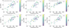 |
Fig. 1 Molecular abundances (X(x) = N(x)/N(H2)) (in logarithmic scale) vs. kinetic temperature. The lines are the result of linear fits whose results are included in the top left corner of each panel. The colors correspond to the volume density of the cores (in cm−3), and the scale is presented in the bar at the right of each panel. |
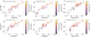 |
Fig. 2 Molecular abundances (X(x) = N(x)/N(H2)) vs. column density (N(x)) presented on a logarithmic scale. The lines are the result of linear fits whose results are included in the top left corner of each panel. The colors correspond to the kinetic temperature measured in the cores, and the scale is presented in the bar at the right of each panel. |
4 Discussion
We first discuss the results we obtained from the comparisons among the molecular abundances, column densities, and physical parameters such as the kinetic temperature and the volume density. The relation between the abundances and temperature (see Fig. 1) shows that the abundance of all analyzed sulfur-bearing species increases with the temperature, that is, the abundances are positively correlated with Tk. This agrees with the results by Fontani et al. (2023) for the SO, SO2, SO+, and H2CS in a sample of high-mass starless cores, high-mass proto-stellar objects, and ultracompact HII regions that were observed with a single-dish telescope.
Based on the linear fittings (see the obtained slopes in Fig. 1), the increment of the molecular abundances with Tk is almost the same for all cases. Thus, we suggest that the chemistry involved in each of the analyzed sulfur-bearing species may have a similar dependence on Tk. This result, obtained for a temperature range from about 20 to 100 K, supports the hypothesis that sulfur may be frozen in the dust grains in dense and cold interstellar regions (Laas & Caselli 2019), and hence, as the temperature rises, the abundance of sulfur-containing molecules increases as well. We cannot discard that the sulfur is already in the gaseous phase and that the temperature increase activates chemical reactions that favor the production of these sulfur-bearing species. The relation we obtained for H2CS is very similar to what was obtained by Chen et al. (2024) from a large sample of massive protoclusters with diverse physical conditions, but in general, they are warmer than the cores investigated here. The core density does not appear to have an effect on the abundance-temperature relation, at least in the density range estimated here, approximately between 106 and 107 cm−3.
The relations between the abundance of a molecular species and its column density (Fig. 2) show an interesting result. The abundance increases with the column density in all cases, which indicates that the column density of the sulfur-containing molecule increases more strongly than N(H2). However, we cannot rule out that N(H2) might be underestimated as a result of dust opacity effects. On the other hand, the relation we obtained for thioformaldehyde from the linear fitting is almost the same as was obtained by Chen et al. (2024) in their sample of massive protoclusters.
Additionally, the panels displayed in Fig. 2 show that the temperature plays an important role in the increasing abundances. Warm cores (orange and yellow points) lie in general above the fitted lines in all cases. This indicates that warm cores have higher molecular abundances than cold cores at the same column density. Our results show that the results by Chen et al. (2024) for the thioformaldehyde also apply to the other sulfur-bearing species, which could be an important point to be taken into account in chemical models for studying the formation of these molecules.
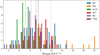 |
Fig. 3 Distribution of the measured line widths ∆v (FWHM) of the sample. The vertical dashed lines are the average values of ∆v of each molecule. In the case of SO and SO+, these averages are almost the same, and the dashed lines appear to overlap. The horizontal axis is truncated at 20 km s−1 for a better visualization. |
4.1 Comparisons of the molecular abundances
As presented in Fig. E.1, all comparisons of the abundances of the analyzed sulfur-bearing species present a positive correlation. Additionally, the increase in X versus X correlates with the kinetic temperature. This phenomenon shows that as the temperature increases, the abundances also increase, which supports, as mentioned above, the hypothesis that the sulfur is trapped in dust-grain ice mantles in the cold regions. Moreover, based on the good, and in some cases very good, correlation among the abundances (a determination coefficient R2 higher than 0.75, and in some cases about 0.9 in the linear regressions), we can conclude that the chemical processes involved in the formation of all analyzed sulfur-bearing species are probably related.
Interestingly, the correlation between X(SO+) and X(SO) is lowest for all pairs of compared abundances. Thus, when we take into account that a possible route of formation of the SO+ in this type of region is through the SO ionization via cosmic rays (Rivilla et al. 2022), it is likely that as the SO abundance increases, some of these molecules contribute to generating SO+, which would be reflected in a loss of correlation between the abundances of both molecules. Moreover, the fact that the average ∆v of both molecules are the same (see Fig. 3) suggests that both species coincide in the same gas layer.
Fontani et al. (2023) presented relations of the abundances of SO+, NS, SO2, and H2CS with SO and obtained Pearson correlation coefficients (ρ) of 0.62, 0.70, 0.95, and 0.73, respectively. In our case, the corresponding Pearson coefficients ( , where R2 is the determination coefficient of the line regressions presented in Fig. E.1) for these abundance relations are 0.83, 0.87, 0.93, and 0.93, respectively. All are higher than those presented by Fontani and collaborators, except for ρ of the X(SO2)/X(SO) relation. The two values are almost the same in this case. Our sample contains sources in earlier evolutionary stages than the sample studied by Fontani et al. (2023), which might explain the better correlation among the abundances we found. This might indicate that these molecules can have a similar chemical origin in these early stages (e.g., the sulfur freeze-out from the dust grains). These correlations among the abundances would then decrease as the cores evolve because the chemistry becomes more complex.
Finally, the obtained values of the X(SO2)/X(SO) ratio for our sample of cores agree with what is yielded by chemical models of a core that is chemically evolved about 105 yr for a temperature of 60 K (see Wakelam et al. 2011). The average measured temperature of our sample is 65 K. Even though we cannot know the chemical ages of the cores in the analyzed sample accurately, we can suggest that our observational results may support the use of this abundance ratio as a chemical clock, as was proposed by the authors.
4.2 Line width comparisons
The obtained ∆v values for the sulfur-bearing molecules are quite similar to those obtained, also from interferometric observations of sulfur species, toward others molecular cores (el Akel et al. 2022; Chen et al. 2024). In this large sample of sources, we must be careful with comparisons with other sources in the literature in different stages of evolution. The clumps in which the analyzed cores are embedded are cataloged as early star-forming regions. However, it is likely that this sample of clumps is not fully uniform. It might exhibit variations in evolutionary stage. As mention above, the ∆v (FWHM) can be used to analyze the location or distribution of the molecular species in different gaseous layers with different dynamics within the cores (Sanhueza et al. 2012; Yu & Wang 2015; Fontani et al. 2023; Martinez & Paron 2024).
Figure E.2 shows that the line widths ∆v (FWHM) of all molecular species are positively correlated, and although it is not well defined, this correlation is in general accompanied by a temperature increase. None of the displayed ∆v comparisons are close to the y = x locus, and only the relation between the line widths of 34SO and NS approaches the unity line slightly. This behavior indicates that the different molecules trace gas with different dynamics or turbulence conditions in general.
In particular, the correlation between H2CS and NS (ρ = 0.93) is excellent, but the NS line widths are systematically larger. When we assume that the ∆v in our sample of cores mainly reflects turbulence, this would indicate that NS traces the same gaseous layer as H2CS, but also receives some contribution from more turbulent material. This agrees with the fact that the correlation between the abundances of these two molecules is one of the highest in the sample (ρ = 0.97; see Fig. E.1). The correlations of ∆v of H2CS and NS with the O-bearing species are generally poor (ρ < 0.7), except for the relation between NS and SO, which have ρ = 0.78. We note that the four O-bearing species have larger ∆v than the other molecular species, indicating that they may be associated with warmer and more turbulent gas. Figs. 3 and E.2 show that the oxygen-containing species trace the most turbulent gas. However, the correlations among them are quite poor, indicating that they may arise from different gaseous layers in the cores. In particular, SO2 is probably located in the innermost region, which is more affected by a possible incipient central compact source, while SO and 34SO could be located farther away. The nature of SO+ is elusive. It presents the poorest correlation with the remaining oxygen-containing species. In addition, its ∆v are generally larger than those of 34SO, but this is not evident when comparing with SO and SO2.
We suggest that H2CS and NS are associated with quiescent gas, likely from the outer envelope of the cores, and NS probably located somewhat more internally than H2CS. The comparison between the FWHM ∆v of these species presents the best correlation, which coincides with the high correlation in the comparison of their abundances. This indicates that the physics and chemistry traced by the two molecular species is probably similar.
The oxygen-containing species may trace inner gas and are probably more affected by incipient star-forming processes. In particular, SO2 traces the warmer and innermost regions. Our results agree well with those obtained by Fontani et al. (2023), who found that the C- and N-bearing species are associated with the quiescent gas in the extended envelope of the sources, while O-bearing species are located in inner regions of the cores. The phenomenon that S- and O-bearing molecules are associated with more turbulent gas was also observed by other authors (see, e.g., Artur de la Villarmois et al. 2019; Garufi et al. 2022; Artur de la Villarmois et al. 2023).
5 Summary and conclusions
We investigated the sulfur-bearing molecules 34SO, SO2, NS, SO, SO+, and H2CS toward 37 molecular cores that are embedded in a sample of infrared-quiet ATLASGAL sources, presumably in very early stages of star formation. Based on the submillimeter continuum emission and methanol lines, the cores were characterized in density and temperature, and the corresponding H2 column densities were derived. The high detection rate of the sulfur-bearing species allowed us to perform a statistical study that is useful for investigating the early sulfur chemistry in dense regions of the ISM. The main results and conclusions are summarized below.
(1) We observed that all the estimated abundances of the analyzed sulfur-bearing species increase in a similar way with increasing gas temperature. This supports the hypothesis that sulfur may be frozen in the dust grains in dense and cold interstellar regions, and hence, as the temperature rises, the abundance of sulfur-containing molecules also increases. It cannot be discarded that the sulfur is already present in the gaseous phase and that the temperature increase activates some new chemical routes of formation of these sulfur-bearing species that increase their abundances. Additionally, we suggest that the chemistry involved in the formation of each of the analyzed sulfur-bearing species may have a similar dependence on Tk, at least in the range from 20 to 100 K.
(2) We found that the warmer cores of our sample have a higher molecular abundances than the colder cores at the same column density for all molecular species. This complements a previous study of thioformaldehyde and indicates that this behavior between the abundances and column densities also applies to the other sulfur-bearing species. This might be a point to be taken into account in chemical models studying the formation of these molecules.
(3) The molecular abundance comparisons presented high correlations in general. When we compare our results with previous similar works done toward more evolved sources, we can conclude that the sulfur-bearing species we analyzed probably have the same chemical origin in the very early stages of the cores. This explains the high correlations. As the cores evolve, the correlations among the molecular abundances decrease, indicating that chemistry becomes more complex.
(4) Based on the analysis of the FWHM ∆v of the molecular lines, we suggest that the analyzed molecules with oxygen content (34SO, SO, SO+, and SO2) may be associated with warmer and more turbulent gas than the other molecules. Our results indicate that the H2CS and NS are associated with more quiescent gas, probably in the external envelopes of the cores, and the O-bearing species are probably located in the inner regions.
(5) In particular, NS and H2CS are strongly correlated in the FWHM ∆v and abundance comparisons. This may indicate that the physics and chemistry traced by the two molecular species are similar.
Finally, we point out that we presented a work with an important piece of information regarding the sulfur chemistry in the earliest stages of the molecular cores, probably pre-stellar cores. This work not only complements recent previous similar works done toward more evolved sources, but also provides quantitative information about abundances that might be useful in chemical models for explaining the sulfur chemistry in the ISM.
Data availability
Some appendices are available at Zenodo: https://doi.org/10.5281/zenodo.14036845
Acknowledgements
We would like to thank to the anonymous referee for her/his useful suggestions and corrections that improved our manuscript. N.C.M. is a doctoral fellow of CONICET. M.O., A.P., and S.P. are members of the Carrera del Investigador Científico of CONICET, Argentina. A.A., M.B., C.C., and T.H. are part of our citizen science project Ciencia Popular2. This work was partially supported by the Argentina grants PIP 2021 11220200100012 and PICT 2021-GRF-TII-00061 awarded by CONICET and ANPCYT. This paper makes use of the following ALMA data: ADS/JAO.ALMA#2017.1.00914.S ALMA is a partnership of ESO (representing its member states), NSF (USA) and NINS (Japan), together with NRC (Canada), MOST and ASIAA (Taiwan), and KASI (Republic of Korea), in cooperation with the Republic of Chile. The Joint ALMA Observatory is operated by ESO, AUI/NRAO and NAOJ. The National Radio Astronomy Observatory is a facility of the National Science Foundation operated under cooperative agreement by Associated Universities, Inc.
Appendix A Source sample
Table A.1 presents the ATLASGAL sources sample and the analyzed cores.
ATLASGAL sources sample and selected cores.
Appendix B Calculation of optical depths
To evaluate the optically thin assumption used to calculate the column densities, we computed the optical depth (τ) of the molecular lines in all cores from the following equation (e.g. Mangum & Shirley 2015):
 (B.1)
(B.1)
where Tpeak is the peak of the emission (values in the ‘Peak’ columns in Tables F1 and F2 converted to K; available on Zenodo3), ϕ the beam filling factor assumed to be 1, and J(T) = hν/k (exp(hν/kT)−1)−1 with Tex = 20 K, and Tbg = 2.73 K. The calculated values of T are presented in Table B.1.
Almost all values of τ are << 1, showing that the lines are indeed optically thin. Some values slightly larger than the unity (see cores 29 and 30 for the H2CS and SO) could affect to the calculated column density in a factor about 2 (using the optical depth correction of τ/(1 −exp(−τ)), which does not change any result.
Line optical depths.
Appendix C Calculation of Trot from the CH3OH
Table C.1 presents the integrated emission from the CH3OH 7(1,7)–6(1, 6)++ (at 335.582 GHz, Eu = 78.97 K) and 12(1,11)-12(0,12)−+ (at 336.865 GHz, Eu = 197.07 K) lines used to estimate temperatures. Such integrated intensities, obtained from Gaussian fittings (for an example see Fig. G4 available on Zenodo3), were used to construct rotational diagrams following Goldsmith & Langer (1999). By assuming LTE conditions, optically thin lines, and a beam filling factor equal to the unity, we can estimate the rotational temperatures (Trot). This analysis is based on a derivation of the Boltzmann equation,
 (C.1)
(C.1)
where Nu represents the molecular column density of the upper level of the transition, gu the total degeneracy of the upper level, Ntot the total column density of the molecule, Qrot the rotational partition function, and k the Boltzmann constant.
Following Miao et al. (1995), for interferometric observations, the left-hand side of Eq. C.1 can be estimated from
 (C.2)
(C.2)
where θa and θb are the major and minor axes of the clean beam, respectively, W is the integrated intensity, gk and gl are the K-level and reduced nuclear spin degeneracies, ν0 is the rest frequency of the line, Sul is the line strength of the transition, and µ0 is the permanent dipole moment of the molecule. The free parameters, (Ntot/Qrot) and Trot were determined by a linear fitting to Eq. C.1. The obtained Trot values are those included in Table D.2 as  .
.
The Trot was estimated by assuming optically thin lines (e.g. van der Tak et al. 2000). However, we consider the possibility of high optical depths in the used CH3OH lines. Thus, following Goldsmith & Langer (1999) and Purcell et al. (2006), we compute the opacity correction factors for the Nu of both lines. We observe that in the cases that it makes sense to apply such a correction, it modifies the Nu value in a similar way for both transitions, and therefore it does not affect the Trot estimation.
CH3OH integrated emission lines.
Appendix D Obtained parameters
Table D.1 displays the obtained column densities of the sulfur-bearing molecular species, and Table D.2 presents some measured and derived core parameters.
LTE column densities (×1013 cm−2).
Measured and derived core parameters.
Appendix E Molecular abundances and measured ∆v FHWM relations
Figures E.1 and E.2 present the relations among the molecular abundances and the measured ∆v FHWM of the sulfur-bearing species, respectively.
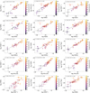 |
Fig. E.1 Comparison of the molecular abundances of all analyzed molecules, presented in logarithmic scale. The lines are the result of linear fittings whose results are included at the top left corner of each panel. The colors correspond to the kinetic temperature measured in the cores, and the scale is presented in the bar at the right of each panel. |
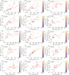 |
Fig. E.2 Comparison of the ∆v FWHM of the molecular lines. The points are color-coded based on the kinetic temperature measured in the cores. The dashed gray line represents the y = x locus. The Pearson correlation coefficient (ρ) is displayed in each panel. |
References
- Amano, T., Amano, T., & Warner, H. E. 1991, J. Mol. Spectrosc., 146, 519 [NASA ADS] [CrossRef] [Google Scholar]
- Artur de la Villarmois, E., Kristensen, L. E., & Jørgensen, J. K. 2019, A&A, 627, A37 [EDP Sciences] [Google Scholar]
- Artur de la Villarmois, E., Guzmán, V. V., Yang, Y. L., Zhang, Y., & Sakai, N. 2023, A&A, 678, A124 [NASA ADS] [CrossRef] [EDP Sciences] [Google Scholar]
- Belov, S. P., Tretyakov, M. Y., Kozin, I. N., et al. 1998, J. Mol. Spectrosc., 191, 17 [NASA ADS] [CrossRef] [Google Scholar]
- Chen, L., Qin, S.-L., Liu, T., et al. 2024, ApJ, 962, 13 [NASA ADS] [CrossRef] [Google Scholar]
- Clark, W. W., & De Lucia, F. C. 1976, J. Mol. Spectrosc., 60, 332 [CrossRef] [Google Scholar]
- Csengeri, T., Bontemps, S., Wyrowski, F., et al. 2017, A&A, 601, A60 [NASA ADS] [CrossRef] [EDP Sciences] [Google Scholar]
- el Akel, M., Kristensen, L. E., Le Gal, R., et al. 2022, A&A, 659, A100 [CrossRef] [EDP Sciences] [Google Scholar]
- Fontani, F., Roueff, E., Colzi, L., & Caselli, P. 2023, A&A, 680, A58 [NASA ADS] [CrossRef] [EDP Sciences] [Google Scholar]
- Fuente, A., Rivière-Marichalar, P., Beitia-Antero, L., et al. 2023, A&A, 670, A114 [NASA ADS] [CrossRef] [EDP Sciences] [Google Scholar]
- Garufi, A., Podio, L., Codella, C., et al. 2022, A&A, 658, A104 [CrossRef] [EDP Sciences] [Google Scholar]
- Goicoechea, J. R., Pety, J., Gerin, M., et al. 2006, A&A, 456, 565 [NASA ADS] [CrossRef] [EDP Sciences] [Google Scholar]
- Goldsmith, P. F., & Langer, W. D. 1999, ApJ, 517, 209 [Google Scholar]
- Gorai, P., Bhat, B., Sil, M., et al. 2020, ApJ, 895, 86 [Google Scholar]
- Hily-Blant, P., Pineau des Forêts, G., Faure, A., & Lique, F. 2022, A&A, 658, A168 [NASA ADS] [CrossRef] [EDP Sciences] [Google Scholar]
- Kauffmann, J., Bertoldi, F., Bourke, T. L., Evans, N. J., I., & Lee, C. W. 2008, A&A, 487, 993 [NASA ADS] [CrossRef] [EDP Sciences] [Google Scholar]
- Laas, J. C., & Caselli, P. 2019, A&A, 624, A108 [NASA ADS] [CrossRef] [EDP Sciences] [Google Scholar]
- Lee, S. K., Ozeki, H., & Saito, S. 1995, ApJS, 98, 351 [NASA ADS] [CrossRef] [Google Scholar]
- Lovas, F. J. 1978, J. Phys. Chem. Ref. Data, 7, 1445 [CrossRef] [Google Scholar]
- Maeda, A., Medvedev, I. R., Winnewisser, M., et al. 2008, ApJS, 176, 543 [NASA ADS] [CrossRef] [Google Scholar]
- Mangum, J. G., & Shirley, Y. L. 2015, PASP, 127, 266 [Google Scholar]
- Martinez, N. C., & Paron, S. 2024, RA&A, 24, 015007 [Google Scholar]
- Miao, Y., Mehringer, D. M., Kuan, Y.-J., & Snyder, L. E. 1995, ApJ, 445, L59 [NASA ADS] [CrossRef] [Google Scholar]
- Müller, H. S. P., Schlöder, F., Stutzki, J., & Winnewisser, G. 2005, J. Mol. Struct., 742, 215 [Google Scholar]
- Pineau des Forets, G., Roueff, E., & Flower, D. R. 1986, MNRAS, 223, 743 [CrossRef] [Google Scholar]
- Purcell, C. R., Balasubramanyam, R., Burton, M. G., et al. 2006, MNRAS, 367, 553 [Google Scholar]
- Rivière-Marichalar, P., Fuente, A., Goicoechea, J. R., et al. 2019, A&A, 628, A16 [Google Scholar]
- Rivilla, V. M., García De La Concepción, J., Jiménez-Serra, I., et al. 2022, Front. Astron. Space Sci., 9, 829288 [NASA ADS] [CrossRef] [Google Scholar]
- Sanhueza, P., Jackson, J. M., Foster, J. B., et al. 2012, ApJ, 756, 60 [Google Scholar]
- Shingledecker, C. N., Lamberts, T., Laas, J. C., et al. 2020, ApJ, 888, 52 [Google Scholar]
- Tiemann, E. 1974, J. Phys. Chem. Ref. Data, 3, 259 [CrossRef] [Google Scholar]
- Turner, B. E. 1995, ApJ, 455, 556 [NASA ADS] [CrossRef] [Google Scholar]
- Urquhart, J. S., König, C., Giannetti, A., et al. 2018, MNRAS, 473, 1059 [Google Scholar]
- van der Tak, F. F. S., van Dishoeck, E. F., & Caselli, P. 2000, A&A, 361, 327 [NASA ADS] [Google Scholar]
- Vastel, C., Quénard, D., Le Gal, R., et al. 2018, MNRAS, 478, 5514 [Google Scholar]
- Wakelam, V., Caselli, P., Ceccarelli, C., Herbst, E., & Castets, A. 2004, A&A, 422, 159 [NASA ADS] [CrossRef] [EDP Sciences] [Google Scholar]
- Wakelam, V., Hersant, F., & Herpin, F. 2011, A&A, 529, A112 [NASA ADS] [CrossRef] [EDP Sciences] [Google Scholar]
- Wienen, M., Wyrowski, F., Schuller, F., et al. 2012, A&A, 544, A146 [NASA ADS] [CrossRef] [EDP Sciences] [Google Scholar]
- Woods, P. M., Occhiogrosso, A., Viti, S., et al. 2015, MNRAS, 450, 1256 [Google Scholar]
- Yu, N., & Wang, J.-J. 2015, MNRAS, 451, 2507 [NASA ADS] [CrossRef] [Google Scholar]
All Tables
All Figures
|
Fig. 1 Molecular abundances (X(x) = N(x)/N(H2)) (in logarithmic scale) vs. kinetic temperature. The lines are the result of linear fits whose results are included in the top left corner of each panel. The colors correspond to the volume density of the cores (in cm−3), and the scale is presented in the bar at the right of each panel. |
| In the text | |
|
Fig. 2 Molecular abundances (X(x) = N(x)/N(H2)) vs. column density (N(x)) presented on a logarithmic scale. The lines are the result of linear fits whose results are included in the top left corner of each panel. The colors correspond to the kinetic temperature measured in the cores, and the scale is presented in the bar at the right of each panel. |
| In the text | |
|
Fig. 3 Distribution of the measured line widths ∆v (FWHM) of the sample. The vertical dashed lines are the average values of ∆v of each molecule. In the case of SO and SO+, these averages are almost the same, and the dashed lines appear to overlap. The horizontal axis is truncated at 20 km s−1 for a better visualization. |
| In the text | |
|
Fig. E.1 Comparison of the molecular abundances of all analyzed molecules, presented in logarithmic scale. The lines are the result of linear fittings whose results are included at the top left corner of each panel. The colors correspond to the kinetic temperature measured in the cores, and the scale is presented in the bar at the right of each panel. |
| In the text | |
|
Fig. E.2 Comparison of the ∆v FWHM of the molecular lines. The points are color-coded based on the kinetic temperature measured in the cores. The dashed gray line represents the y = x locus. The Pearson correlation coefficient (ρ) is displayed in each panel. |
| In the text | |
Current usage metrics show cumulative count of Article Views (full-text article views including HTML views, PDF and ePub downloads, according to the available data) and Abstracts Views on Vision4Press platform.
Data correspond to usage on the plateform after 2015. The current usage metrics is available 48-96 hours after online publication and is updated daily on week days.
Initial download of the metrics may take a while.