| Issue |
A&A
Volume 692, December 2024
|
|
|---|---|---|
| Article Number | A242 | |
| Number of page(s) | 12 | |
| Section | Galactic structure, stellar clusters and populations | |
| DOI | https://doi.org/10.1051/0004-6361/202452274 | |
| Published online | 17 December 2024 | |
Improving constraints on the extended mass distribution in the Galactic center with stellar orbits
1
LESIA, Observatoire de Paris, Université PSL, CNRS, Sorbonne Université, Université de Paris,
5 place Jules Janssen,
92195
Meudon,
France
2
Max Planck Institute for Extraterrestrial Physics,
Giessenbachstraße 1,
85748
Garching,
Germany
3
Univ. Grenoble Alpes, CNRS, IPAG,
38000
Grenoble,
France
4
European Southern Observatory,
Karl-Schwarzschild-Straße 2,
85748
Garching,
Germany
5
Max Planck Institute for Astronomy,
Königstuhl 17,
69117
Heidelberg,
Germany
6
1st Institute of Physics, University of Cologne,
Zülpicher Straße 77,
50937
Cologne,
Germany
7
CENTRA – Centro de Astrofísica e Gravitação, IST, Universidade de Lisboa,
1049-001
Lisboa,
Portugal
8
Universidade de Lisboa – Faculdade de Ciências, Campo Grande,
1749-016
Lisboa,
Portugal
9
European Southern Observatory, Casilla
19001,
Santiago 19,
Chile
10
Faculdade de Engenharia, Universidade do Porto, rua Dr. Roberto Frias,
4200-465
Porto,
Portugal
11
Departments of Physics & Astronomy, Le Conte Hall, University of California,
Berkeley,
CA
94720,
USA
12
Max Planck Institute for Astrophysics,
Karl-Schwarzschild-Straße 1,
85748
Garching,
Germany
13
Max Planck Institute for Radio Astronomy,
auf dem Hügel 69,
53121
Bonn,
Germany
14
Institute of Multidisciplinary Mathematics, Universitat Politècnica de València,
València,
Spain
15
Kavli Institute for Astronomy and Astrophysics,
Beijing,
China
16
Advanced Concepts Team, ESA, TEC-SF, ESTEC,
Keplerlaan 1,
2201
AZ
Noordwijk,
The Netherlands
17
Niels Bohr International Academy, Niels Bohr Institute,
Blegdamsvej 17,
2100
Copenhagen,
Denmark
18
ORIGINS Excellence Cluster,
Boltzmannstraße 2,
85748
Garching,
Germany
19
Department of Physics, Technical University of Munich,
85748
Garching,
Germany
20
Higgs Centre for Theoretical Physics,
Edinburgh,
UK
21
Department of Physics, Sapienza, University of Rome,
P.le A. Moro 5,
00185
Rome,
Italy
22
School of Physics and Materials Science, Guangzhou University,
Guangzhou
510006,
PR
China
23
Key Laboratory for Astronomical Observation and Technology of Guangzhou,
510006
Guangzhou,
PR
China
24
Astronomy Science and Technology Research Laboratory of Department of Education of Guangdong Province,
Guangzhou
510006,
PR
China
★★ Corresponding author; This email address is being protected from spambots. You need JavaScript enabled to view it.
Received:
17
September
2024
Accepted:
12
November
2024
Abstract
Studying the orbital motion of stars around Sagittarius A* in the Galactic center provides a unique opportunity to probe the gravitational potential near the supermassive black hole at the heart of our Galaxy. Interferometric data obtained with the GRAVITY instrument at the Very Large Telescope Interferometer (VLTI) since 2016 has allowed us to achieve unprecedented precision in tracking the orbits of these stars. GRAVITY data have been key to detecting the in-plane, prograde Schwarzschild precession of the orbit of the star S2 that is predicted by general relativity. By combining astrometric and spectroscopic data from multiple stars, including S2, S29, S38, and S55 – for which we have data around their time of pericenter passage with GRAVITY – we can now strengthen the significance of this detection to an approximately 10σ confidence level. The prograde precession of S2’s orbit provides valuable insights into the potential presence of an extended mass distribution surrounding Sagittarius A*, which could consist of a dynamically relaxed stellar cusp comprising old stars and stellar remnants, along with a possible dark matter spike. Our analysis, based on two plausible density profiles – a power-law and a Plummer profile – constrains the enclosed mass within the orbit of S2 to be consistent with zero, establishing an upper limit of approximately 1200 M⊙ with a 1σ confidence level. This significantly improves our constraints on the mass distribution in the Galactic center. Our upper limit is very close to the expected value from numerical simulations for a stellar cusp in the Galactic center, leaving little room for a significant enhancement of dark matter density near Sagittarius A*.
Key words: black hole physics / gravitation / instrumentation: interferometers / Galaxy: center
GRAVITY is developed in collaboration by MPE, LESIA of Paris Observatory/CNRS/Sorbonne Université/Univ. Paris Diderot, and IPAG of Université Grenoble Alpes/CNRS, MPIA, Univ. of Cologne, CENTRA – Centro de Astrofisica e Gravitação, and ESO.
© The Authors 2024
 Open Access article, published by EDP Sciences, under the terms of the Creative Commons Attribution License (https://creativecommons.org/licenses/by/4.0), which permits unrestricted use, distribution, and reproduction in any medium, provided the original work is properly cited.
This article is published in open access under the Subscribe to Open model.
Open Access funding provided by Max Planck Society.
1 Introduction
Since 2016, the GRAVITY interferometer at ESO’s Very Large Telescope (GRAVITY Collaboration 2017) has allowed us to obtain astrometric data with unprecedented accuracy (reaching in the best cases a 1σ uncertainty of 30 μas) of the S-stars orbiting around Sagittarius A* (Sgr A*) in the Galactic center (GC). This has turned them into a powerful tool to investigate the gravitational potential near the supermassive black hole (SMBH) at the center of our Galaxy, reaching distances from Sgr A* down to about a thousand times its Schwarzschild radius (RS). Furthermore, astrometric and polarimetric observations of flares from Sgr A* with GRAVITY have revealed that the mass inside the flares’ radius of a few RS is consistent with the black hole mass measured from stellar orbits (GRAVITY Collaboration 2018b, 2023a). This, together with the radio-VLBI image of Sgr A* Event Horizon Telescope Collaboration 2022), confirms that Sgr A* is a SMBH beyond any reasonable doubt.
For the S2 star, due to its short orbital period of 16 years and its brightness (mK ≈ 14), astrometric data are available for two complete orbital revolutions around Sgr A*, while spectroscopic data cover one and a half revolutions (Schödel et al. 2002; Ghez et al. 2003, 2008; Gillessen et al. 2017). At the pericenter, S2 reaches a distance of ~1400 RS from the SMBH with a speed of 7700 km s−1 ≃ 0.026 c. Monitoring the star’s motion on the sky and radial velocity with GRAVITY and SINFONI around the time of the pericenter passage in 2018, crucial data were obtained in order to detect the first-order effects in the post-Newtonian (PN) expansion of general relativity (GR) on its orbital motion. The first one is the gravitational red-shift of spectral lines, which was detected together with the transverse Doppler effect, predicted by special relativity, with a ≈10σ significance in GRAVITY Collaboration (2018a) and a ≈5σ significance in Do et al. (2019). GRAVITY Collaboration (2019) improved the significance of the detection to ≈20σ. The other effect is the prograde, in-plane precession of the orbit’s pericenter angle; namely, the Schwarzschild precession (SP). It corresponds to an advance of ![Mathematical equation: $\[\delta \varphi_{S ~c h w}=\frac{3 \pi R_{S}}{a\left(1{-}e^{2}\right)}\]$](/articles/aa/full_html/2024/12/aa52274-24/aa52274-24-eq1.png) per orbit, which for S2 is equal to 12.1 arcmin per orbit in the prograde direction. In GRAVITY Collaboration (2020), this effect was detected at the 5σ level, and improved in GRAVITY Collaboration (2022) to ≈7σ by combining the data of S2 with data of the stars S29, S38, and S55, which could be observed with GRAVITY around the time of their pericenter passage and whose pericenter distances are comparable to that of S2.
per orbit, which for S2 is equal to 12.1 arcmin per orbit in the prograde direction. In GRAVITY Collaboration (2020), this effect was detected at the 5σ level, and improved in GRAVITY Collaboration (2022) to ≈7σ by combining the data of S2 with data of the stars S29, S38, and S55, which could be observed with GRAVITY around the time of their pericenter passage and whose pericenter distances are comparable to that of S2.
The Lense-Thirring effect, caused by the spin of the central SMBH, appears at a 1.5 PN order and gives both an additional contribution to the in-plane precession and a precession of the orbital plane (Merritt et al. 2010). We define ![Mathematical equation: $\[A_{L T}= 4 \pi \chi~(\frac{R_{S}}{2 a(1{-}e^{2})})^{3 / 2}\]$](/articles/aa/full_html/2024/12/aa52274-24/aa52274-24-eq2.png) , which for S2 is equal to 0.11 arcminutes. Consequently, the in-plane precession per orbit becomes δφKerr = δφS chw − 2ALT cos(i), while the precession per orbit of the orbital plane is given by δΦKerr = ALT, where χ is the dimensionless spin of the SMBH (with 0 ≤ χ ≤ 1) and i is the angle between the direction of the SMBH spin and that of the stellar orbital angular momentum. The effect is thus at least 50 times smaller than the SP, assuming a SMBH with maximum spin, and is out of reach for current measurements. In order to measure the spin of Sgr A*, we would need to observe a star with a pericenter distance that is at least three times smaller than that of S2, given the astrometric accuracy achievable with GRAVITY (Waisberg et al. 2018; Capuzzo-Dolcetta & Sadun-Bordoni 2023).
, which for S2 is equal to 0.11 arcminutes. Consequently, the in-plane precession per orbit becomes δφKerr = δφS chw − 2ALT cos(i), while the precession per orbit of the orbital plane is given by δΦKerr = ALT, where χ is the dimensionless spin of the SMBH (with 0 ≤ χ ≤ 1) and i is the angle between the direction of the SMBH spin and that of the stellar orbital angular momentum. The effect is thus at least 50 times smaller than the SP, assuming a SMBH with maximum spin, and is out of reach for current measurements. In order to measure the spin of Sgr A*, we would need to observe a star with a pericenter distance that is at least three times smaller than that of S2, given the astrometric accuracy achievable with GRAVITY (Waisberg et al. 2018; Capuzzo-Dolcetta & Sadun-Bordoni 2023).
Any extended mass distribution around Sgr A*, following a spherically symmetric density profile, would add a retrograde precession of the stellar orbits, counteracting the prograde SP (GRAVITY Collaboration 2020, 2022). This mass distribution is expected to be composed mainly of a dynamically relaxed cusp of old stars and stellar remnants. Peebles (1972); Frank & Rees (1976); Bahcall & Wolf (1976) first addressed the problem of the distribution of stars around a central massive BH. Bahcall & Wolf (1976) found that a single-mass stellar population around a central massive BH reaches a stationary density distribution over the two-body relaxation timescale, which is a power law, ρ(r) ∝ rs, with slope s = −1.75. In the GC, the old stellar population can be approximately represented by light stars with masses around 1 M⊙ and heavier stellar black holes with masses around 10 M⊙ (Alexander 2017). For such a population, mass segregation occurs, where heavier objects tend to concentrate toward the center due to dynamical interactions with lighter objects. The mass-segregation solution for the steady-state distribution of stars around a massive BH is derived in Alexander & Hopman (2009). It has two branches, weak and strong segregation, based on the dominance of heavier or lighter objects in the scattering interactions. In the weak segregation branch, the heavy objects settle into a power-law distribution with a slope of −1.75, while the lighter objects exhibit a shallower profile with a slope of −1.5, as was already heuristically derived in Bahcall & Wolf (1977). Conversely, the strong segregation branch results in steeper slopes and a larger difference between the light and heavy masses. The heavy masses settle into a much steeper cusp with −2.75 ≲ s ≲ −2, while the light masses settle into a cusp with −1.75 ≲ s ≲ −1.5. Preto & Amaro-Seoane (2010) provided a clear realization through N-body simulations of the strong mass segregation solution, showing also that the stellar cusp can develop on timescales that are much shorter than the relaxation time, which is shorter than the Hubble time for the GC (Alexander & Hopman 2009; Genzel et al. 2010). In Linial & Sari (2022), it is argued that weak segregation must exist interior to a certain break radius, rB, where the massive population dominates the scattering, while for radii larger than rB the light objects dominate the scattering and strong segregation occurs.
The existence of such a stellar cusp in the GC is also validated by the observational results of Gallego-Cano et al. (2018) and Schödel et al. (2018) for the distribution of giant, subgiant, and main-sequence stars within the central few parsecs. They find that the density distribution of the light objects is shallower than s = −1.5, being compatible with a power-law with slope between −1.4 and −1.15. This is impossible in the steady state, Bahcall & Wolf framework in order to maintain an equilibrium distribution, but could be explained by a number of factors, such as stellar collisions (Rose & MacLeod 2024), taking into account the complex star formation history of the nuclear star cluster (Baumgardt et al. 2018), or by diffusion in angular momentum leading to tidal disruptions; namely, diffusion into the loss cone (Zhang & Amaro-Seoane 2024). Red giant stars, instead, do not show a cusp but a distribution that appears to flatten toward the central 0.3 pc (Buchholz et al. 2009; Do et al. 2009; Bartko et al. 2010; Gallego-Cano et al. 2018), possibly due to the stripping of red giant envelopes due to the interaction with a star-forming disk (Amaro-Seoane & Chen 2014).
In addition to the stellar cusp, an intermediate-mass black hole (IMBH) companion of Sgr A* could be present in the GC. It has been shown that an IMBH enclosed within the orbit of S2 can only have a mass of <103 M⊙ (GRAVITY Collaboration 2023b; Will et al. 2023). Moreover, it was predicted by Gondolo & Silk (1999) that dark matter particles could be accreted by the SMBH to form a dense spike, increasing the dark matter density in the GC by up to ten orders of magnitude with respect to the expected density in the case of a Navarro–Frenk–White (NFW) profile. In this scenario, the spike could contribute to the extended mass distribution around Sgr A*, while in the absence of such a spike, the contribution of dark matter within the radial range of the S-stars’ orbits would be negligible under an NFW profile. The dark matter spike would also follow a power-law distribution, ρ(r) ∝ rs, with slope −2.5 < s < −2.25 in the case of a generalized NFW profile (Gondolo & Silk 1999; Shen et al. 2024). Another possibility that has been investigated is that dark matter could exist in the form of an ultralight scalar field or a massive vector field cloud that clusters around Sgr A* (Foschi et al. 2023; GRAVITY Collaboration 2024), or as a compact fermion ball supported by degeneracy pressure (Viollier et al. 1993; Argüelles et al. 2019; Becerra-Vergara et al. 2020).
Additionally, a deviation from general relativity, such as the one introduced by massive gravity theories or f(R)-gravity, could modify the gravitational potential through a Yukawa-like correction in the Newtonian limit, adding an additional precession of the stellar orbits to the prograde SP and the retrograde precession induced by an extended mass distribution (Hees et al. 2017; De Martino et al. 2021; Tan & Lu 2024; Jovanović et al. 2024a,b). For the specific case of massive gravity, the additional precession would be prograde and equal to ![Mathematical equation: $\[\delta \varphi_{Y}=\pi \sqrt{1-e^{2}} \frac{a^{2}}{\lambda^{2}}\]$](/articles/aa/full_html/2024/12/aa52274-24/aa52274-24-eq3.png) (Jovanović et al. 2024a), where
(Jovanović et al. 2024a), where ![Mathematical equation: $\[\lambda=\frac{\hbar}{m_{g} c}\]$](/articles/aa/full_html/2024/12/aa52274-24/aa52274-24-eq4.png) is the Compton wave-length of the massive graviton, mg the mass of the graviton, and ℏ the reduced Planck constant. From the observed precession of the S2 star, it is thus possible to derive a lower limit on λ and an upper limit on mg, as is done in Hees et al. (2017); Jovanović et al. (2024a,b).
is the Compton wave-length of the massive graviton, mg the mass of the graviton, and ℏ the reduced Planck constant. From the observed precession of the S2 star, it is thus possible to derive a lower limit on λ and an upper limit on mg, as is done in Hees et al. (2017); Jovanović et al. (2024a,b).
In GRAVITY Collaboration (2022), the 1σ upper limit on any extended mass distributed within the orbit of S2 is found to be ≈3000 M⊙, assuming a Plummer density profile (Plummer 1911). In this paper, we use S-star data, including one more year of GRAVITY observations, in order to improve and extend the analysis conducted in GRAVITY Collaboration (2022). Our goal is to enhance the significance of the SP detection and to improve the observational constraints on the extended mass distribution around Sgr A*, comparing these results with theoretical models. In Section 2, we describe our dataset. We give our results for the SP detection in Section 3 and for the extended mass distribution in Section 4. In Section 5, we summarize our conclusions.
2 Observations
We describe in GRAVITY Collaboration (2022) how interferometric astrometry with GRAVITY confers many advantages over single-telescope AO imaging. Most importantly, it allows us to reach a much higher angular resolution and astrometric accuracy and to be significantly less affected by confusion noise. In this paper, we add one more year of GRAVITY data (up to September of 2022) for the stars S2, S29, S38, and S55 with respect to GRAVITY Collaboration (2022). In addition, since April 2023, the Enhanced Resolution Imager and Spectrograph (ERIS) has started to be operational at the VLT (Davies et al. 2023). This has made it possible, after the decommissioning of SINFONI (Eisenhauer et al. 2005) in 2019, to resume spectroscopic observations of the S-stars, with a new state-of-the-art AO system and a much higher spectral resolution (R ~ 10 000, compared to R ~ 4000 of SINFONI). In this paper, we add to the long-standing SINFONI dataset the first radial velocity data points obtained with ERIS, during the commissioning phase in 2022.
For the analysis conducted in this paper, we used the following dataset:
For S2, we used 128 NACO and 82 GRAVITY data points for the astrometry, and 92 SINFONI, 3 Keck, 2 NACO, 4 GNIRS/GEMINI, and 3 ERIS radial velocity measurements. These data cover the time span of 1992.2-2022.7.
For S29, we used 66 NACO (2002.3-2019.7) and 29 GRAVITY data points (2019.6-2022.7) for the astrometry. We dropped a significant fraction of the available NACO data, which have been affected by confusion events. We also used 17 SINFONI and 2 GNIRS radial velocity measurements (2007.6-2021.4).
For S38, we used 110 NACO (2004.2-2018.6) and 23 GRAVITY (2021.2-2022.7) data points for the astrometry, and 8 SINFONI, 2 Keck, and 1 ERIS data points for the radial velocity (2008.3-2022.4).
For S55, we used 42 NACO (2004.5-2013.6) and 27 GRAVITY (2021.2-2022.6) astrometric data points, and 2 SINFONI radial velocity data points (2014).
We also used the NACO and GRAVITY astrometric data and the SINFONI radial velocity data for other two stars: S24 and S42. For five other stars, S1, S4, S9, S21, and S13, we only used NACO and SINFONI data.
Figure 1 illustrates the orbits of all these stars. Details on the analysis of GRAVITY data can be found in Appendix A of GRAVITY Collaboration (2020). The analysis of spectroscopic data is described in Habibi et al. (2017) and GRAVITY Collaboration (2019).
3 Schwarzschild precession of the orbit of S2
3.1 Method
To test whether the orbits of S-stars are well described by a Schwarzschild orbit around Sgr A*, we modeled their acceleration given by a first-order PN approximation of GR for a massless test particle (Will 1993) and multiplied the 1PN terms by a factor, fS P, such that fS P = 0 corresponds to a Keplerian closed (non-precessing) orbit and fS P = 1 to a GR Schwarzschild orbit, with a prograde precession of the orbit’s pericenter angle. The parameter, fS P, was then used as a fitting parameter, together with the mass of and distance to the central SMBH, m• and R0, five coordinates (x0, y0, vx0, vy0, vz0) describing the position on the sky and three-dimensional velocity of Sgr A* in the AO imaging and spectroscopic reference frame, and six orbital parameters (a, e, i, ω, Ω, t0) for each star that we used in the orbital fit, describing the initial osculating Kepler orbit.
The orbital fitting was done using either a Levenberg-Marquardt χ2 minimization algorithm or a (Metropolis-Hastings) Markov chain Monte Carlo (MCMC) analysis, using 200000 realizations (for more details, see GRAVITY Collaboration 2018a, 2019, 2020).
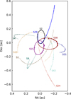 |
Fig. 1 Orbits for the set of 11 S-stars that have been used in this paper. Highlighted are the four most relevant stars to constrain the gravitational potential around Sgr A*: S2, S29, S38, and S55. |
3.2 Results
Here, we used the complete dataset of the stars S2, S29, S38, and S55 (Section 2) to obtain the best possible constraint on fS P. As is noted in GRAVITY Collaboration (2020, 2022), the NACO zero points x0, y0, vx0, vy0 are partially degenerate with fS P. To mitigate this degeneracy, we used data from seven additional S-stars (see Section 2 and Figure 1), performing a combined Keplerian fit to obtain an estimate for x0, y0, vx0, vy0. We then combined the result for x0, y0, vx0, vy0 obtained from the stellar orbits with the constraints from the NACO astrometry of flares and the prior from the construction of the AO reference frame (Plewa et al. 2015), in order to derive a prior for these parameters (see Appendix B).
Fitting the data of S2 using this prior for the NACO zero points, we obtain fS P = 0.918 ± 0.128 (MCMC fS P = 0.911 ± 0.131). The result improves when fitting the data of S2 together with S29, S38, and S55. In fact, these stars passed through the pericenter between 2021 and 2023, allowing us to observe them around the time of their pericenter passage with GRAVITY (GRAVITY Collaboration 2022). Their pericenter distances are comparable to that of S2, ranging from 1200 RS to 2800 RS, providing crucial data to improve our constraints on the gravitational potential around Sgr A*. With this comprehensive dataset, we obtain fS P = 1.135 ± 0.110 (MCMC fS P = 1.133 ± 0.113). The significance of the SP detection has thus increased from ≈7σ of GRAVITY Collaboration (2022) to ≈10σ. It is therefore strikingly evident that the orbit of S2 is, with ever stronger significance, described by a Schwarzschild orbit around Sgr A*, exhibiting a prograde, in-plane precession of its pericenter angle. In the upper panel of Figure 2, we show the NACO and GRAVITY astrometric data of S2, highlighting the effect of the SP by comparing the GRAVITY 2021–2022 data with the NACO data from 2005, obtained one orbital period earlier. In the bottom panel, we show the averaged S2 residual data obtained with GRAVITY and NACO, after subtracting the Newtonian component of the best-fit Schwarzschild orbit. The data points follow the Schwarzschild orbit predicted by GR, which corresponds to the loopy red line in the plot.
For the first time, we have also been able to measure the SP of S2’s orbit using only the GRAVITY astrometric data and the radial velocity data, due to the coverage of almost half of S2’s orbit with GRAVITY. This allows us to completely exclude the NACO data from the fit and remove the NACO reference frame parameters x0, y0, vx0, vy0, since with GRAVITY we can directly measure the separation vector between Sgr A* and S2. Fitting the orbit of S2, we obtain fS P = 1.016 ± 0.226 (MCMC fS P = 1.024 ± 0.260), indicating a measurement of the SP with a ≈4σ confidence. This leads to a less significant detection than the one achieved by including the NACO data in the analysis, despite fitting four fewer parameters, which helps to reduce some degeneracies. In Appendix A, we attempt to predict how much we shall be able to improve our constraint on fS P by continuing to monitor the orbit of S2 with GRAVITY and ERIS, carrying out mock observations. We show that GRAVITY data taken in the coming years, until the S2 star reaches the next apocenter passage in 2026, will only moderately improve the SP detection. Additionally, we show that the NACO imaging data will still be key in the near future in order to achieve the best possible constraint on fS P, at least until S2 has gone through the next pericenter passage in 2034.
 |
Fig. 2 The SP in the orbit of S2 around Sgr A*. Top: astrometric data of S2 obtained from 1992 to the end of 2022, together with the best-fitting orbit. The SHARP and NACO data are in black, while the GRAVITY data are in red. Sgr A* is located at (0,0), marked by a black cross. A zoom-in shows the effect of the prograde SP, comparing the GRAVITY 2021–2022 data with the NACO 2005 data. Bottom: residuals in RA and Dec between the best-fit Schwarzschild orbit (fS P = 1) and the Newtonian component of the same orbit (fS P = 0). In the plot, the Schwarzschild orbit predicted by GR corresponds to the loopy red curve. The corresponding residual GRAVITY data with respect to the Newtonian orbit are represented by red circles, and the NACO data by a black circle. The GRAVITY data points follow the Schwarzschild orbit predicted by GR. GRAVITY data are averages of several epochs. The NACO data have been averaged into one single data point. |
4 The extended mass distribution around Sgr A*
4.1 Method
To test the existence of an extended mass distribution around Sgr A*, we fixed fS P = 1 (we assume a 1PN approximation of GR) and we modeled the extended mass distribution using a spherically symmetric density profile, ρ(r). In this case, the motion of stars is not only due to the SMBH gravitational potential but also to the potential generated by this additional mass distribution, which gives an additional term to the stars acceleration and causes a retrograde precession of their orbits.
We chose to test two plausible density profiles:
-
The power-law profile
![Mathematical equation: $\[$\rho(r)=\rho_{0}\left(\frac{r}{r_{0}}\right)^{s}$,\]$](/articles/aa/full_html/2024/12/aa52274-24/aa52274-24-eq5.png) (1)
(1)where r0 is a length scale for the radial coordinate (we fixed it to r0 = 40 mpc), ρ0 is the density at r = r0, and s is the slope of the power law. Integrating, we obtain the enclosed mass as a function of the radius:
![Mathematical equation: $\[m(r)=\frac{4 \pi \rho_{0}}{3+s}\left(\frac{r^{3+s}}{r_{0}^{s}}\right).\]$](/articles/aa/full_html/2024/12/aa52274-24/aa52274-24-eq6.png) (2)
(2)This is the distribution expected in the case of a stellar cusp, with a slope of −2.75 ≲ s ≤ −1.5 depending on the mass of the stellar population and whether weak or strong mass segregation occurs (Alexander & Hopman 2009; Preto & Amaro-Seoane 2010), and in the case of a dark matter spike, with a slope of −2.5 < s < −2.25 (Shen et al. 2024). We investigated this profile, varying the slope in the range −3 < s ≤ 0. We thus explored a range of possible slopes for the density distribution, from a constant density profile, ρ = ρ0 = const, for s = 0, to progressively steeper distributions with divergent central density for s < 0.
-
The Plummer profile (Plummer 1911) is
![Mathematical equation: $\[\rho(r)=\rho_{0}\left[1+\left(\frac{r}{a}\right)^{2}\right]^{-5 / 2},\]$](/articles/aa/full_html/2024/12/aa52274-24/aa52274-24-eq7.png) (3)
(3)where a is the scale radius of the distribution, such that
![Mathematical equation: $\[\rho(r=a)=\frac{\rho_{0}}{2^{5 / 2}}\]$](/articles/aa/full_html/2024/12/aa52274-24/aa52274-24-eq8.png) , and ρ0 is the (finite) central density.
, and ρ0 is the (finite) central density.Integrating, we obtain the enclosed mass profile:
![Mathematical equation: $\[\begin{equation*}m(r)=\frac{4}{3} \pi \rho_{0} a^{3} \frac{(r / a)^{3}}{\left[1+(r / a)^{2}\right]^{3 / 2}}\end{equation*}.\]$](/articles/aa/full_html/2024/12/aa52274-24/aa52274-24-eq9.png) (4)
(4)The total mass of the distribution is equal to
![Mathematical equation: $\[m_{t o t}=\frac{4}{3} \pi \rho_{0} a^{3}\]$](/articles/aa/full_html/2024/12/aa52274-24/aa52274-24-eq10.png) . We investigated this profile, varying the scale radius in the range 0 < a ≤ 40 mpc, going from very compact to progressively broader distributions, and thus also exploring the possibility that the density distribution reaches a plateau (a finite value ρ(r = 0) = ρ0) at the center.
. We investigated this profile, varying the scale radius in the range 0 < a ≤ 40 mpc, going from very compact to progressively broader distributions, and thus also exploring the possibility that the density distribution reaches a plateau (a finite value ρ(r = 0) = ρ0) at the center.
The procedure we adopted is the following. We parametrized both distributions by defining ρ0 = fpowm• for the power law and ![Mathematical equation: $\[\rho_{0}=\frac{f_{pl}m_\bullet}{\frac{4}{3} \pi a^{3}}\]$](/articles/aa/full_html/2024/12/aa52274-24/aa52274-24-eq11.png) for Plummer. In the first case, we fixed the slope, s, of the power law to different values in the interval (−3, 0] and fit for the parameter fpow, again together with m•, R0, the reference frame parameters, x0, y0, vx0, vy0, vz0, and six orbital parameters (a, e, i, ω, Ω, t0) per star. In the second case, we fixed the scale radius, a, of the Plummer profile to different values in the interval (0, 40] mpc and fit for fpl together with the other parameters. The orbital fitting was done using an MCMC analysis with 200000 realizations. We did not allow the parameters s (for the power law) and a (for Plummer) to vary freely in the fit alongside fpow and fpl because doing so significantly increases the computational cost of the MCMC analysis, making it challenging to effectively explore the entire parameter space. It was assumed as a prior that fpow ≥ 0 and fpl ≥ 0, ensuring that the density is ρ(r) ≥ 0 for every value of r. Then, we converted the resulting posterior distribution of the parameters fpow and fpl into a distribution on the parameter Mencl,S2 = m(rperi,S2 < r < rapo,S2); namely, the enclosed mass within the orbit of S2 (see Appendix B), where the pericenter distance of S2 is rperi,S2 ~ 0.6 mpc and the apocenter distance is rapo,S2 ~ 9.4 mpc. We focused on the enclosed mass within S2’s orbit because it corresponds to the radial range over which the data used in the orbital fits lie. Presenting the results on the total mass of the Plummer distribution or the total mass of the power-law distribution within a radius of rcut > > rapo,S2 is less relevant, as they depend on the chosen model for the density distribution and cannot be effectively constrained by our data. In addition, the mass enclosed within S2 pericenter m(rperi,S2) is degenerate with the SMBH mass, m•, and for very steep distributions it is not well constrained with our data (see Appendix B).
for Plummer. In the first case, we fixed the slope, s, of the power law to different values in the interval (−3, 0] and fit for the parameter fpow, again together with m•, R0, the reference frame parameters, x0, y0, vx0, vy0, vz0, and six orbital parameters (a, e, i, ω, Ω, t0) per star. In the second case, we fixed the scale radius, a, of the Plummer profile to different values in the interval (0, 40] mpc and fit for fpl together with the other parameters. The orbital fitting was done using an MCMC analysis with 200000 realizations. We did not allow the parameters s (for the power law) and a (for Plummer) to vary freely in the fit alongside fpow and fpl because doing so significantly increases the computational cost of the MCMC analysis, making it challenging to effectively explore the entire parameter space. It was assumed as a prior that fpow ≥ 0 and fpl ≥ 0, ensuring that the density is ρ(r) ≥ 0 for every value of r. Then, we converted the resulting posterior distribution of the parameters fpow and fpl into a distribution on the parameter Mencl,S2 = m(rperi,S2 < r < rapo,S2); namely, the enclosed mass within the orbit of S2 (see Appendix B), where the pericenter distance of S2 is rperi,S2 ~ 0.6 mpc and the apocenter distance is rapo,S2 ~ 9.4 mpc. We focused on the enclosed mass within S2’s orbit because it corresponds to the radial range over which the data used in the orbital fits lie. Presenting the results on the total mass of the Plummer distribution or the total mass of the power-law distribution within a radius of rcut > > rapo,S2 is less relevant, as they depend on the chosen model for the density distribution and cannot be effectively constrained by our data. In addition, the mass enclosed within S2 pericenter m(rperi,S2) is degenerate with the SMBH mass, m•, and for very steep distributions it is not well constrained with our data (see Appendix B).
4.2 Results
The fact that we observe a prograde, in-plane precession of S2’s orbit, as is predicted by GR, implies that we can get strong constraints on the potential existence of an extended mass component distributed around Sgr A*. In fact, if such an extended mass component were present, it would induce a retrograde precession of S2’s orbit, counteracting the prograde SP.
To test for the existence of an extended mass distribution around Sgr A*, we followed the procedure described in Section 4.1, performing a multi-star fit with the stars S2, S29, S38, and S55. For each star, we utilized the complete dataset available (Section 2), using both NACO and GRAVITY astrometric data. We imposed a prior on the NACO zero points x0, y0, vx0, vy0, as in Section 3.2.
As was expected, we derived strong constraints on the enclosed mass within S2’s orbit, Mencl,S2. The enclosed mass is compatible with zero, indicating that the orbits of the stars can be accurately described by Schwarzschild orbits without any extended mass surrounding the SMBH. In Figure 3, we plot the 1σ and 3σ upper limits (corresponding to 68.3% c.i. and 99.7% c.i., see Appendix B) on this parameter, as a function of the power-law slope (s) for a power-law distribution, and as a function of the Plummer scale radius (a) for a Plummer distribution. We find that we cannot distinguish between different density profiles, as a power law with different slopes and a Plummer profile with different core radii fit the data equally well (we find no significant difference in χ2). However, regardless of the specific density profile, we can reach a general conclusion. The 1σ upper limit on the enclosed mass within the orbit of S2 is lower than ≈1200 M⊙ for a power law with slope s ≲ −1.2 and for a Plummer profile with scale radius a ≲ 8 mpc, which corresponds approximately to the apocenter distance of S2. These constraints represent a significant improvement over the results found in GRAVITY Collaboration (2022), where the 1σ upper limit on any extended mass within S2’s apocenter was found to be ≈3000 M⊙. In addition, this can be translated into an upper limit on the amount of retrograde precession induced by the mass distribution, which we find to be ≲ 1 arcmin per orbit and which is subdominant with respect to the prograde SP of ~12 arcmin per orbit. We emphasize that the data from S29, S38, and S55 are crucial for achieving such strong constraints (see Appendix B for a comparison with the results obtained from fitting the data of S2 only).
 |
Fig. 3 Upper limit on the enclosed mass within the orbit of S2 for an extended mass distribution around Sgr A*. We tested two plausible density profiles for the mass distribution: a power-law profile with varying slope (panel a) and a Plummer profile with varying scale radius (panel b). In red, we plot the 1σ upper limit and in blue the 3σ upper limit, derived from a multi-star fit using data from the stars S2, S29, S38, and S55. Independently of the density profile, the enclosed mass within S2’s orbit is consistently compatible with zero. We set a strong upper limit of approximately 1200 M⊙ with a 1σ confidence level, for reasonable choices of the slope of the power law (s < −1.2) and the scale radius of the Plummer profile (a ≲ 8 mpc). |
4.3 Comparison with theoretical models for the stellar cusp
We now compare our derived upper limit on the enclosed mass within the orbit of S2 to what is predicted for a dynamically relaxed stellar cusp in the GC. Zhang & Amaro-Seoane (2024) present a new Monte Carlo method that allows one to study the dynamical evolution of a star cluster with multiple mass components in the vicinity of a SMBH in a galactic nucleus. The code calculates the two-body relaxation process based on two-dimensional (energy and angular momentum) Fokker-Planck equations and includes the effects of the loss cone, giving a more realistic result that what can be obtained in the steady-state framework of Bahcall & Wolf (1976, 1977); Alexander & Hopman (2009). Assuming a population of light objects with ml = 1 M⊙ and a population of heavy remnants with mh = 10 M⊙, they find consistent results with the mass segregation solution described in Alexander & Hopman (2009); Preto & Amaro-Seoane (2010). The heavy black holes sink toward the center due to dynamical friction and follow a steeper density profile, as is expected from mass segregation, reaching a slope between ~−2.3 and ~−1.7 in the inner regions. The light objects follow the expected slope of −1.5 if loss cone effects are ignored, while their density profile becomes shallower in the inner regions if the effects of the loss cone are included, reaching a slope of ~−1.3.
Here, we used an updated version of the code (Zhang & Amaro-Seoane, in prep.) that includes the potential from the stars and not only that of the central SMBH, in the calculation of the two-body relaxation of the energy and angular momentum of the particles in the simulation. This is particularly important for an accurate estimate of the density profile beyond the radius of influence of the SMBH, but also for the flux of particles into the loss cone. We considered a model with five components; namely, distinguishing between populations of stars of ms = 1 M⊙, brown dwarfs of mbd = 0.05 M⊙, white dwarfs of mwd = 0.6 M⊙, neutron stars of mns = 1.4 M⊙, and stellar black holes of mbh = 10 M⊙, as in Zhang & Amaro-Seoane (2024). The fraction of brown dwarfs with respect to the stars at the beginning of the simulation is fbd = 0.2, the fraction of white dwarfs is fwd = 0.1, neutron stars fns = 0.01, and stellar black holes fbh = 0.001. The initial density profile in the simulation is a Dehnen model (Dehnen 1993) with γ = 1, total mass Mcl = 3.2 × 10⁷ M⊙, and scale radius ra = 1.86 pc. We let the system evolve for one relaxation time and find that the radius at which the total enclosed mass in the simulation equals 2m• — the radius of influence of the SMBH (Merritt 2013) – is r = 3.9 pc, consistent with findings from Chatzopoulos et al. (2014); Feldmeier-Krause et al. (2016). In Figure 4, we show the enclosed mass profile resulting from the simulations as a function of distance from the SMBH, comparing it with our observational results. The enclosed mass within the orbit of S2 predicted by the simulations is mencl,S2 = 1210 M⊙, which is in agreement with our upper limit mencl,S2 ≲ 1200 M⊙ for a power-law density profile with slope s < −1.2. A similar result is obtained when considering a model with just two components; namely, stars of 1 M⊙ and stellar black holes of 10 M⊙, giving a total enclosed mass within S2’s orbit of mencl,S2 = 1300 M⊙. Moreover, the simulations indicate that stellar mass black holes dominate the mass distribution in this region, contributing significantly to the total mass enclosed within the orbit of S2.
Since our upper limit is extremely close to the value predicted by simulations for a dynamically relaxed stellar cusp, we conclude that there is no substantial evidence for a significant enhancement of dark matter density near Sagittarius A*. However, it is important to note that, in principle, our orbital fits cannot distinguish between the mass contributions from the stellar cusp and a potential dark matter spike, as both are expected to follow similar power-law density distributions.
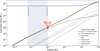 |
Fig. 4 Enclosed mass in the GC as a function of radius derived from numerical simulations, using an updated version of the code from Zhang & Amaro-Seoane (2024), for a model that includes stellar black holes, neutron stars, white dwarfs, brown dwarfs, and stars. The dashed colored lines show the predicted enclosed mass of each individual component, while the solid black line shows the total predicted enclosed mass considering all components. The predicted enclosed mass within S2’s orbit is in agreement with our 1σ upper limit of ≈1200 M⊙, indicated by the red square. The solid blue line shows the sum of the mass of Sgr A* to the total predicted enclosed mass. The shaded blue region illustrates the radial range of the orbit of S2. |
4.4 Note on the granularity of the stellar cusp
Our upper limit on the enclosed mass within S2’s orbit of mencl,S2 ≲ 1200 M⊙ is low enough to raise questions about whether modeling the extended mass distribution as a smooth, spherically symmetric density profile is a valid approximation. Figure 4 illustrates that, due to mass segregation, stellar black holes dominate the extended mass distribution within S2’s orbit. Therefore, we considered a scenario in which a finite number of bodies generate the extended potential by distributing the total enclosed mass among N objects of equal mass. This configuration can lead to deviations in the orbital motion of S-stars compared to a smooth density distribution, as spherical symmetry is broken and scattering events may occur. In this case, there is not only in-plane precession but also precession of the orbital plane, as was discussed in Merritt et al. (2010).
An extreme case occurs when all the extended mass is concentrated in a single object, specifically an IMBH companion to Sgr A*. It has been shown that an IMBH within the orbit of S2 can only have a mass of <103 M⊙, in order to be compatible with observations (GRAVITY Collaboration 2023b; Will et al. 2023).
We assume that a cluster of 100 point-mass particles, each with a mass of 10 M⊙, is distributed within the apocenter of S2, following a power-law density distribution of the form ρ(r) ∝ r−2. We further assume that these particles are fixed in space and do not interact with one another. To assess the impact of this distribution on the orbit of S2, we conducted 100 mock observations of one full orbit of S2 around Sgr A* and the surrounding field objects, where each simulation corresponds to a different sampling of the field object positions to ensure adequate statistics. We then fit each simulated orbit for the fS P parameter (see Section 3.1), obtaining a distribution with a mean and median of fS P = 0.94, a standard deviation of 0.01, and a range of 0.09. When repeating this experiment with a cluster of 20 point-mass particles, each of 50 M⊙, we obtain a distribution with a mean and median of fS P = 0.95, a standard deviation of 0.03, and a range of 0.23.
These results suggest that a distribution of stellar black holes around Sgr A* can in principle perturb our measurement of the SP, causing a deviation in S2’s orbit from the expected Schwarzschild orbit. This is an important effect to consider, especially as we achieve increasingly precise measurements of the SP using GRAVITY data, which have led to an error on fS P of ~0.1 (Section 3.2). A detailed treatment of the effects of the granularity of the stellar cusp on stellar orbits is beyond the scope of this paper and will be addressed in detail in a forthcoming publication (Sadun Bordoni et al., in preparation).
5 Conclusions
In this paper, we have improved and extended the analysis conducted in GRAVITY Collaboration (2020, 2022), adding the new interferometric data obtained with GRAVITY in 2022. Particularly valuable, in addition to data for the well-known star S2, are data from the stars S29, S38, and S55. These stars have recently reached the pericenter of their orbits, allowing us to observe them around this critical phase with GRAVITY.
The orbital motions of S2, S29, S38, and S55 are perfectly compatible with Schwarzschild orbits around Sgr A* predicted by GR, exhibiting prograde, in-plane precession of their pericenter angles. By performing a multi-star fit with this data, we have detected the SP of their orbits with a confidence level of approximately ≈10σ, marking a significant improvement over previous findings (GRAVITY Collaboration 2020, 2022).
We establish a stringent upper limit for the mass of any hypothetical extended mass distribution around Sgr A*, which would add a retrograde precession to the orbit of S2, counteracting the prograde, relativistic precession. This mass distribution could be composed of a dynamically relaxed cusp of old stars and stellar remnants and potentially of a dark matter spike. We modeled it with a spherically symmetric density distribution, testing two plausible density profiles; namely, a power law and a Plummer profile. We have found that, independently of the particular density profile, the enclosed mass within S2’s orbit is consistently compatible with zero. We set a strong upper limit of approximately 1200 M⊙ with a 1σ confidence level, significantly improving upon the limits established in GRAVITY Collaboration (2022). Our findings align with theoretical predictions for a dynamically relaxed stellar cusp in the GC, composed of stars, brown dwarfs, white dwarfs, neutron stars, and stellar black holes, according to numerical simulations using an updated version of the code developed in Zhang & Amaro-Seoane (2024). This analysis predicts an enclosed mass of approximately 1210 M⊙ within S2’s orbit. Given that our upper limit is very close to this predicted value, we conclude that we find no evidence for a significant dark matter spike in the GC.
S2 is currently moving toward the apocenter of its orbit, which it will reach in 2026. We expect that GRAVITY data collected in the coming years, combined with ERIS spectroscopy, will further refine our constraints on the extended mass distribution in the GC, as the mass distribution primarily influences stellar orbits in the apocenter half (Heißel et al. 2022). This will allow us to refine the comparison with the theoretical predictions for the stellar cusp, which is of fundamental importance in order to understand the distribution of the faint, old main-sequence stars and subgiants in the GC. These stars are too faint to be currently detected with GRAVITY, but their detection could be in reach of future observations with the GRAVITY+ upgrade at the VLTI (GRAVITY+ Collaboration 2022) and the MICADO instrument at the ELT (Davies et al. 2018). These stars could potentially be in tighter orbits around Sgr A* and could allow us to measure its spin and quadrupole moment. Furthermore, the comparison between our observational constraints and theoretical predictions is also important to better understand the distribution of compact objects in the GC and in galactic nuclei in general. This could offer precious insights in view of the future LISA mission (Amaro-Seoane et al. 2017), which will be able to detect the inspirals of compact objects into SMBHs (EMRIs) (Amaro-Seoane et al. 2007). In fact, the rate of EMRIs depends strongly on the density distribution of compact remnants within ~10 mpc of the central SMBH (Preto & Amaro-Seoane 2010), which corresponds to the apocenter distance of S2 for the GC.
Acknowledgements
We are very grateful to our funding agencies (MPG, ERC, CNRS [PNCG, PNGRAM], DFG, BMBF, Paris Observatory [CS, PhyFOG], Observatoire des Sciences de l’Univers de Grenoble, and the Fundação para a Ciência e Tecnologia), to ESO and the Paranal staff, and to the many scientific and technical staff members in our institutions, who helped to make NACO, SINFONI, and GRAVITY a reality. JS is supported by the Deutsche Forschungsgemeinschaft (DFG, German Research Foundation) under Germany’s Excellence Strategy – EXC-2094 – 390783311. A.A., A.F., P.G. and V.C. were supported by Fundação para a Ciência e a Tecnologia, with grants reference SFRH/BSAB/142940/2018, UIDB/00099/2020 and PTDC/FIS-AST/7002/2020. F.W. has received funding from the European Union’s Horizon 2020 research and innovation programme under grant agreement No 101004719. Based on observations collected at the European Southern Observatory under the ESO programme IDs 109.22ZA.005, 109.22ZA.002, 105.20B2.004, 0103.B-0032(C), 0101.B-0576(E), 0101.B-0576(C).
Appendix A Predicting the improvement on the SP detection with future observations
In order to predict how much we will be able to improve our constraint on the fS P parameter by continuing to monitor the orbit of S2 with GRAVITY and ERIS, we carried out mock observations assuming that we will get, between March and September of each year (GC observing season from Paranal observatory):
10 GRAVITY data points per year with 50 μas astrometric accuracy,
3 radial velocity data points per year with ERIS with 10 km/s accuracy.
We then fit the actual S2 dataset together with the mock dataset and obtain a prediction on the error on fS P in function of time. The result of this analysis is shown in Figure A.1. We compare the case in which we keep the NACO data in the fit with a prior on the reference frame parameters, with the case in which we use GRAVITY data only and we thus remove the reference frame parameters. This shows that GRAVITY data taken in the following years, until the S2 star will reach the next apocenter in 2026, will only moderately improve the SP detection. The predicted error remains then almost constant until ≈2034, namely the time of the next pericenter passage of S2, and starts then to rapidly decrease. This is not surprising, because the SP happens mostly around pericenter (Angélil & Saha 2014; GRAVITY Collaboration 2020; Heißel et al. 2022).
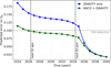 |
Fig. A.1 Predicted error on fS P as a function of time, obtained through mock observations of S2 with GRAVITY and ERIS. The blue points show the result keeping only GRAVITY data in the fit, namely excluding the NACO data and removing the reference frame parameters. The green points show the result keeping both NACO and GRAVITY data. |
This analysis also tells us how valuable the NACO imaging data will still be in the near future, at least until S2 will reach the next pericenter passage in 2034. In fact, Figure A.1 shows that the constraint on fS P will be stronger including NACO data in the orbital fit until a few years after the next pericenter passage of S2. In order to reach the same accuracy that we will be able to get on the SP detection keeping the NACO data in the fit, but using only GRAVITY data and eliminating the NACO zero points x0, y0, vx0, vy0, we would need to wait until ≈2037, when we will have observed two consecutive pericenter passages with GRAVITY.
Appendix B Fit details
Best-fit parameters of the four-star fit determining fS P
In Table B.1 we give the best-fit parameters of the four-star fit determining fS P in Section 3.2.
In Figure B.1 we show an example of posterior distribution on the enclosed mass within S2’s orbit, as derived from an MCMC analysis in the case of a multi-star fit with the stars S2, S29, S38 and S55. The 1σ upper limit on the enclosed mass corresponds to a 68.3% confidence level, the 3σ upper limit to a 99.7% confidence level.
In Figure B.2 we highlight that the mass enclosed within S2 pericenter is not well constrained with our data, as it is degenerate with the SMBH mass in the fitting. It depends severely on the steepness of the density profile.
In Figure B.3 we show the constraints on the enclosed mass within S2’s orbit, obtained fitting the orbit of S2 only. Comparing Figure 3 with Figure B.3 it is immediately noticeable that a multi-star fit, namely fitting the data of S2 together with S29, S38 and S55, helps to obtain a much tighter constraint on the enclosed mass within S2’s orbit than fitting the data of S2 only. The constraint is stronger for more compact distributions, namely for a steep power-law distribution and a Plummer profile with a small scale radius, and it becomes weaker for shallower distributions. This can be understood by translating the result on the enclosed mass into the amount of retrograde precession caused by this mass on the stellar orbits: the shallower the distribution, the larger is the amount of extended mass that can lie within the orbit of S2 inducing the same amount of retrograde precession.
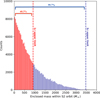 |
Fig. B.1 Example of posterior distribution on the enclosed mass within S2’s orbit, for an MCMC analysis with 200 000 realizations, showing how the 1σ and 3σ upper limits are derived. This example corresponds to the case of a multi-star fit with the stars S2, S29, S38, S55 for a power-law density profile with slope s = −2.2. |
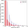 |
Fig. B.2 Enclosed mass within S2 pericenter for an extended mass distribution following a power-law density profile with varying slope. In red is plotted the 1σ upper limit and in blue the 3σ upper limit on this parameter, derived from a multi-star fit with the stars S2, S29, S38, S55. |
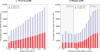 |
Fig. B.3 Enclosed mass within S2’s orbit for an extended mass distribution following a power-law density profile with varying slope (a) and a Plummer density profile with varying scale radius (b). In red is plotted the 1σ upper limit and in blue the 3σ upper limit on this parameter, derived fitting the orbit of S2. |
References
- Alexander, T. 2017, ARA&A, 55, 17 [NASA ADS] [CrossRef] [Google Scholar]
- Alexander, T., & Hopman, C. 2009, ApJ, 697, 1861 [NASA ADS] [CrossRef] [Google Scholar]
- Amaro-Seoane, P., & Chen, X. 2014, ApJ, 781, L18 [NASA ADS] [CrossRef] [Google Scholar]
- Amaro-Seoane, P., Gair, J. R., Freitag, M., et al. 2007, Class. Quant. Grav., 24, R113 [NASA ADS] [CrossRef] [Google Scholar]
- Amaro-Seoane, P., Audley, H., Babak, S., et al. 2017, Laser Interferometer Space Antenna (ESA PUBLICATIONS DIVISION C/O ESTEC), submitted to ESA on January 13th in response to the call for missions for the L3 slot in the Cosmic Vision Programme [Google Scholar]
- Angélil, R., & Saha, P. 2014, MNRAS, 444, 3780 [CrossRef] [Google Scholar]
- Argüelles, C. R., Krut, A., Rueda, J. A., & Ruffini, R. 2019, Int. J. Mod. Phys. D, 28, 1943003 [CrossRef] [Google Scholar]
- Bahcall, J. N., & Wolf, R. A. 1976, ApJ, 209, 214 [NASA ADS] [CrossRef] [Google Scholar]
- Bahcall, J. N., & Wolf, R. A. 1977, ApJ, 216, 883 [NASA ADS] [CrossRef] [Google Scholar]
- Bartko, H., Martins, F., Trippe, S., et al. 2010, ApJ, 708, 834 [Google Scholar]
- Baumgardt, H., Amaro-Seoane, P., & Schödel, R. 2018, A&A, 609, A28 [NASA ADS] [CrossRef] [EDP Sciences] [Google Scholar]
- Becerra-Vergara, E. A., Argüelles, C. R., Krut, A., Rueda, J. A., & Ruffini, R. 2020, A&A, 641, A34 [NASA ADS] [CrossRef] [EDP Sciences] [Google Scholar]
- Buchholz, R. M., Schödel, R., & Eckart, A. 2009, A&A, 499, 483 [NASA ADS] [CrossRef] [EDP Sciences] [Google Scholar]
- Capuzzo-Dolcetta, R., & Sadun-Bordoni, M. 2023, MNRAS, 522, 5828 [NASA ADS] [CrossRef] [Google Scholar]
- Chatzopoulos, S., Fritz, T. K., Gerhard, O., et al. 2014, MNRAS, 447, 948 [Google Scholar]
- Davies, R., Alves, J., Clénet, Y., et al. 2018, SPIE Conf. Ser., 10702, 107021S [NASA ADS] [Google Scholar]
- Davies, R., Absil, O., Agapito, G., et al. 2023, A&A, 674, A207 [NASA ADS] [CrossRef] [EDP Sciences] [Google Scholar]
- Dehnen, W. 1993, MNRAS, 265, 250 [NASA ADS] [CrossRef] [Google Scholar]
- De Martino, I., della Monica, R., & De Laurentis, M. 2021, Phys. Rev. D, 104, L101502 [NASA ADS] [CrossRef] [Google Scholar]
- Do, T., Ghez, A. M., Morris, M. R., et al. 2009, ApJ, 703, 1323 [NASA ADS] [CrossRef] [Google Scholar]
- Do, T., Hees, A., Ghez, A., et al. 2019, Science, 365, 664 [Google Scholar]
- Eisenhauer, F., Genzel, R., Alexander, T., et al. 2005, ApJ, 628, 246 [Google Scholar]
- Event Horizon Telescope Collaboration 2022, ApJ, 930, L12 [NASA ADS] [CrossRef] [Google Scholar]
- Feldmeier-Krause, A., Zhu, L., Neumayer, N., et al. 2016, MNRAS, 466, 4040 [Google Scholar]
- Foschi, A., Abuter, R., Aimar, N., et al. 2023, MNRAS, 524, 1075 [Google Scholar]
- Frank, J., & Rees, M. J. 1976, MNRAS, 176, 633 [NASA ADS] [CrossRef] [Google Scholar]
- Gallego-Cano, E., Schödel, R., Dong, H., et al. 2018, A&A, 609, A26 [NASA ADS] [CrossRef] [EDP Sciences] [Google Scholar]
- Genzel, R., Eisenhauer, F., & Gillessen, S. 2010, Rev. Mod. Phys., 82, 3121 [Google Scholar]
- Ghez, A. M., Duchêne, G., Matthews, K., et al. 2003, ApJ, 586, L127 [Google Scholar]
- Ghez, A. M., Salim, S., Weinberg, N. N., et al. 2008, ApJ, 689, 1044 [Google Scholar]
- Gillessen, S., Plewa, P. M., Eisenhauer, F., et al. 2017, ApJ, 837, 30 [Google Scholar]
- Gondolo, P., & Silk, J. 1999, Phys. Rev. Lett., 83, 1719 [Google Scholar]
- GRAVITY Collaboration (Abuter, R., et al.) 2017, A&A, 602, A94 [NASA ADS] [CrossRef] [EDP Sciences] [Google Scholar]
- GRAVITY Collaboration (Abuter, R., et al.) 2018a, A&A, 615, L15 [NASA ADS] [CrossRef] [EDP Sciences] [Google Scholar]
- GRAVITY Collaboration (Abuter, R., et al.) 2018b, A&A, 618, L10 [NASA ADS] [CrossRef] [EDP Sciences] [Google Scholar]
- GRAVITY Collaboration (Abuter, R., et al.) 2019, A&A, 625, L10 [NASA ADS] [CrossRef] [EDP Sciences] [Google Scholar]
- GRAVITY Collaboration (Abuter, R., et al.) 2020, A&A, 636, L5 [NASA ADS] [CrossRef] [EDP Sciences] [Google Scholar]
- GRAVITY Collaboration (Abuter, R., et al.) 2022, A&A, 657, L12 [NASA ADS] [CrossRef] [Google Scholar]
- GRAVITY Collaboration (Abuter, R., et al.) 2023a, A&A, 677, L10 [NASA ADS] [CrossRef] [EDP Sciences] [Google Scholar]
- GRAVITY Collaboration (Straub, O., et al.) 2023b, A&A, 672, A63 [NASA ADS] [CrossRef] [EDP Sciences] [Google Scholar]
- GRAVITY Collaboration 2024, MNRAS, 530, 3740 [Google Scholar]
- GRAVITY+ Collaboration (Abuter, R., et al.) 2022, The Messenger, 189, 17 [NASA ADS] [Google Scholar]
- Habibi, M., Gillessen, S., Martins, F., et al. 2017, ApJ, 847, 120 [Google Scholar]
- Hees, A., Do, T., Ghez, A. M., et al. 2017, Phys. Rev. Lett., 118, 211101 [Google Scholar]
- Heiel, G., Paumard, T., Perrin, G., & Vincent, F. 2022, A&A, 660, A13 [NASA ADS] [CrossRef] [EDP Sciences] [Google Scholar]
- Jovanović, P., Borka Jovanović, V., Borka, D., & Zakharov, A. F. 2024a, Symmetry, 16, 397 [Google Scholar]
- Jovanović, P., Borka Jovanović, V., Borka, D., & Zakharov, A. F. 2024b, Phys. Rev. D, 109, 064046 [Google Scholar]
- Linial, I., & Sari, R. 2022, ApJ, 940, 101 [CrossRef] [Google Scholar]
- Merritt, D. 2013, Dynamics and Evolution of Galactic Nuclei (Princeton: Princeton University Press) [Google Scholar]
- Merritt, D., Alexander, T., Mikkola, S., & Will, C. M. 2010, Phys. Rev. D, 81, 062002 [Google Scholar]
- Peebles, P. J. E. 1972, ApJ, 178, 371 [NASA ADS] [CrossRef] [Google Scholar]
- Plewa, P. M., Gillessen, S., Eisenhauer, F., et al. 2015, MNRAS, 453, 3234 [Google Scholar]
- Plummer, H. C. 1911, MNRAS, 71, 460 [Google Scholar]
- Preto, M., & Amaro-Seoane, P. 2010, ApJ, 708, L42 [NASA ADS] [CrossRef] [Google Scholar]
- Rose, S. C., & MacLeod, M. 2024, ApJ, 963, L17 [NASA ADS] [CrossRef] [Google Scholar]
- Schödel, R., Ott, T., Genzel, R., et al. 2002, Nature, 419, 694 [Google Scholar]
- Schödel, R., Gallego-Cano, E., Dong, H., et al. 2018, A&A, 609, A27 [Google Scholar]
- Shen, Z.-Q., Yuan, G.-W., Jiang, C.-Z., et al. 2024, MNRAS, 527, 3196 [Google Scholar]
- Tan, Y., & Lu, Y. 2024, Phys. Rev. D, 109, 044047 [Google Scholar]
- Viollier, R., Trautmann, D., & Tupper, G. 1993, Phys. Lett. B, 306, 79 [Google Scholar]
- Waisberg, I., Dexter, J., Gillessen, S., et al. 2018, MNRAS, 476, 3600 [NASA ADS] [CrossRef] [Google Scholar]
- Will, C. M. 1993, Theory and Experiment in Gravitational Physics (Cambridge University Press) [CrossRef] [Google Scholar]
- Will, C. M., Naoz, S., Hees, A., et al. 2023, ApJ, 959, 58 [NASA ADS] [CrossRef] [Google Scholar]
- Zhang, F., & Amaro-Seoane, P. 2024, ApJ, 961, 232 [NASA ADS] [CrossRef] [Google Scholar]
All Tables
All Figures
|
Fig. 1 Orbits for the set of 11 S-stars that have been used in this paper. Highlighted are the four most relevant stars to constrain the gravitational potential around Sgr A*: S2, S29, S38, and S55. |
| In the text | |
|
Fig. 2 The SP in the orbit of S2 around Sgr A*. Top: astrometric data of S2 obtained from 1992 to the end of 2022, together with the best-fitting orbit. The SHARP and NACO data are in black, while the GRAVITY data are in red. Sgr A* is located at (0,0), marked by a black cross. A zoom-in shows the effect of the prograde SP, comparing the GRAVITY 2021–2022 data with the NACO 2005 data. Bottom: residuals in RA and Dec between the best-fit Schwarzschild orbit (fS P = 1) and the Newtonian component of the same orbit (fS P = 0). In the plot, the Schwarzschild orbit predicted by GR corresponds to the loopy red curve. The corresponding residual GRAVITY data with respect to the Newtonian orbit are represented by red circles, and the NACO data by a black circle. The GRAVITY data points follow the Schwarzschild orbit predicted by GR. GRAVITY data are averages of several epochs. The NACO data have been averaged into one single data point. |
| In the text | |
|
Fig. 3 Upper limit on the enclosed mass within the orbit of S2 for an extended mass distribution around Sgr A*. We tested two plausible density profiles for the mass distribution: a power-law profile with varying slope (panel a) and a Plummer profile with varying scale radius (panel b). In red, we plot the 1σ upper limit and in blue the 3σ upper limit, derived from a multi-star fit using data from the stars S2, S29, S38, and S55. Independently of the density profile, the enclosed mass within S2’s orbit is consistently compatible with zero. We set a strong upper limit of approximately 1200 M⊙ with a 1σ confidence level, for reasonable choices of the slope of the power law (s < −1.2) and the scale radius of the Plummer profile (a ≲ 8 mpc). |
| In the text | |
|
Fig. 4 Enclosed mass in the GC as a function of radius derived from numerical simulations, using an updated version of the code from Zhang & Amaro-Seoane (2024), for a model that includes stellar black holes, neutron stars, white dwarfs, brown dwarfs, and stars. The dashed colored lines show the predicted enclosed mass of each individual component, while the solid black line shows the total predicted enclosed mass considering all components. The predicted enclosed mass within S2’s orbit is in agreement with our 1σ upper limit of ≈1200 M⊙, indicated by the red square. The solid blue line shows the sum of the mass of Sgr A* to the total predicted enclosed mass. The shaded blue region illustrates the radial range of the orbit of S2. |
| In the text | |
|
Fig. A.1 Predicted error on fS P as a function of time, obtained through mock observations of S2 with GRAVITY and ERIS. The blue points show the result keeping only GRAVITY data in the fit, namely excluding the NACO data and removing the reference frame parameters. The green points show the result keeping both NACO and GRAVITY data. |
| In the text | |
|
Fig. B.1 Example of posterior distribution on the enclosed mass within S2’s orbit, for an MCMC analysis with 200 000 realizations, showing how the 1σ and 3σ upper limits are derived. This example corresponds to the case of a multi-star fit with the stars S2, S29, S38, S55 for a power-law density profile with slope s = −2.2. |
| In the text | |
|
Fig. B.2 Enclosed mass within S2 pericenter for an extended mass distribution following a power-law density profile with varying slope. In red is plotted the 1σ upper limit and in blue the 3σ upper limit on this parameter, derived from a multi-star fit with the stars S2, S29, S38, S55. |
| In the text | |
|
Fig. B.3 Enclosed mass within S2’s orbit for an extended mass distribution following a power-law density profile with varying slope (a) and a Plummer density profile with varying scale radius (b). In red is plotted the 1σ upper limit and in blue the 3σ upper limit on this parameter, derived fitting the orbit of S2. |
| In the text | |
Current usage metrics show cumulative count of Article Views (full-text article views including HTML views, PDF and ePub downloads, according to the available data) and Abstracts Views on Vision4Press platform.
Data correspond to usage on the plateform after 2015. The current usage metrics is available 48-96 hours after online publication and is updated daily on week days.
Initial download of the metrics may take a while.