| Issue |
A&A
Volume 698, June 2025
|
|
|---|---|---|
| Article Number | L15 | |
| Number of page(s) | 6 | |
| Section | Letters to the Editor | |
| DOI | https://doi.org/10.1051/0004-6361/202554676 | |
| Published online | 06 June 2025 | |
Letter to the Editor
Exploring the presence of a fifth force at the Galactic Center
1
LIRA, Observatoire de Paris, Université PSL, CNRS, Sorbonne Université, Université de Paris, 5 place Jules Janssen, 92195 Meudon, France
2
Max Planck Institute for Extraterrestrial Physics, Giessenbachstraße 1, 85748 Garching, Germany
3
Univ. Grenoble Alpes, CNRS, IPAG, 38000 Grenoble, France
4
European Southern Observatory, Karl-Schwarzschild-Straße 2, 85748 Garching, Germany
5
Max Planck Institute for Astronomy, Königstuhl 17, 69117 Heidelberg, Germany
6
1st Institute of Physics, University of Cologne, Zülpicher Straße 77, 50937 Cologne, Germany
7
CENTRA – Centro de Astrofísica e Gravitação, IST, Universidade de Lisboa, 1049-001 Lisboa, Portugal
8
Universidade de Lisboa – Faculdade de Ciências, Campo Grande, 1749-016 Lisboa, Portugal
9
European Southern Observatory, Casilla, 19001 Santiago 19, Chile
10
Faculdade de Engenharia, Universidade do Porto, rua Dr. Roberto Frias, 4200-465 Porto, Portugal
11
Departments of Physics & Astronomy, Le Conte Hall, University of California, Berkeley, CA 94720, USA
12
Max Planck Institute for Astrophysics, Karl-Schwarzschild-Straße 1, 85748 Garching, Germany
13
Max Planck Institute for Radio Astronomy, auf dem Hügel 69, 53121 Bonn, Germany
14
Institute of Multidisciplinary Mathematics, Universitat Politècnica de València, València, Spain
15
Center of Gravity, Niels Bohr Institute, Blegdamsvej 17, 2100 Copenhagen, Denmark
16
ORIGINS Excellence Cluster, Boltzmannstraße 2, 85748 Garching, Germany
17
Department of Physics, Technical University of Munich, 85748 Garching, Germany
18
Higgs Centre for Theoretical Physics, Edinburgh, UK
19
Leiden University, 2311 EZ Leiden, The Netherlands
20
The Kavli Institute for Astronomy and Astrophysics, Peking University, Beijing 100871, China
⋆⋆ Corresponding author: This email address is being protected from spambots. You need JavaScript enabled to view it.
Received:
21
March
2025
Accepted:
1
May
2025
Abstract
Aims. We investigate the presence of a Yukawa-like correction to Newtonian gravity at the Galactic Center, leading to a new upper limit on the intensity of such a correction.
Methods. We performed a Markov chain Monte Carlo (MCMC) analysis using the astrometric and spectroscopic data of star S2 collected at the Very Large Telescope by GRAVITY, NACO, and SINFONI instruments, covering the period from 1992 to 2022.
Results. The precision of the GRAVITY instrument allows us to derive the most stringent upper limit at the Galactic Center for the intensity of the Yukawa contribution (∝ αe−λr) of |α|< 0.003 for a scale length of λ = 3 ⋅ 1013 m (∼ 200 AU). This is an improvement on all estimates obtained in previous works by roughly one order of magnitude.
Key words: gravitation / celestial mechanics / Galaxy: center
GRAVITY is developed in collaboration by MPE, LESIA of Paris Observatory/CNRS/Sorbonne Université/Univ. Paris Diderot, and IPAG of Université Grenoble Alpes/CNRS, MPIA, Univ. of Cologne, CENTRA – Centro de Astrofisica e Gravitação, and ESO.
© The Authors 2025
 Open Access article, published by EDP Sciences, under the terms of the Creative Commons Attribution License (https://creativecommons.org/licenses/by/4.0), which permits unrestricted use, distribution, and reproduction in any medium, provided the original work is properly cited.
This article is published in open access under the Subscribe to Open model. This email address is being protected from spambots. You need JavaScript enabled to view it. to support open access publication.
1. Introduction
General relativity (GR) is the most widely recognized theory of gravity today. Its predictions have been extensively tested on Solar System scales and using gravitational waves emission by black holes (BHs) and binary pulsars (Will 2014, 2018a; Nitz et al. 2021). Until now, no significant deviation from GR has been detected in any of these observations. However, it is also known that beyond the regime we are currently able to test experimentally, GR is generally considered insufficient.
Cosmological observations indicate an expanding Universe whose acceleration can only be explained by introducing a cosmological constant ad hoc, which lacks a solid theoretical explanation and raises several issues (Weinberg 1989; Peebles & Ratra 2003). Other observational evidence, such as the rotational curve of galaxies (van Albada et al. 1985; Salucci 2019) or gravitational lensing effects (Massey et al. 2010) indicate the presence of a dark massive component of the Universe, whose nature is still unknown. Furthermore, it is well known that GR lacks a quantum description at high-energy scales and several attempts have been made to create a theory valid at all scales (for a review on the state-of-the-art approaches, see, e.g., Esposito 2011; Kiefer 2023).
One way to address these inconsistencies between theory and experiments is to directly modify GR, giving rise to a plethora of possible extended theories of gravity (ETG). In particular, a Yukawa-like interaction emerges quite naturally in the weak field limit of several ETGs; for instance, scalar-tensor-vector theories (Moffat 2006), massive gravity theories (Visser 1998; Hinterbichler 2012), theories in higher dimensions with Kaluza-Klein compactification (Bars & Visser 1986; Hoyle et al. 2001), massive Brans-Dicke theories (Perivolaropoulos 2010; Alsing et al. 2012), or f(R) theories (Capozziello et al. 2015). However, the so-called “fifth-force” scenario has also made an appearance in a number of specific dark matter models (Frieman & Gradwohl 1991; Gradwohl & Frieman 1992; Carroll et al. 2009).
Due to the importance that a modification of Newtonian gravity would have on our understanding of the Universe, the presence of a Yukawa-like contribution has been repeatedly investigated in the past. The fifth-force intensity is well constrained at Solar System scales via the motion of planets (Konopliv et al. 2011; Hees et al. 2014; Bergé 2017; Will 2018b; Shankaranarayanan & Johnson 2022), from the Lunar Laser Ranging experiment (Hofmann & Müller 2018) and also by making use of the planetary ephemerides (Mariani et al. 2023; Fienga & Minazzoli 2024). Recent constraints have been obtained from asteroids tracking (Tsai et al. 2023, 2024) and test of the weak equivalence principle (Touboul 2022).
The discovery of orbiting stars around the Galactic Center (GC) (Eckart & Genzel 1996; Schödel et al. 2002; Ghez et al. 2003; Gillessen et al. 2009a,b; Sabha 2012), all located within one arcsecond distance from the supermassive black hole (SMBH) Sagittarius A* (Sgr A*), allows us to test GR in a completely different environment from the Solar System.
The importance of looking for a fifth force in the GC lies in the fact that many ETGs that predict a Yukawa-like term also display a screening mechanism that suppresses the fifth force contribution at Solar System scales and prevents its detection. This would explain why it would be yet unobserved, while its effect may be different around SMBHs.
The current constraints on the intensity of a fifth force in the GC come from the analysis of SgrA*’s shadow by the Event Horizon Telescope (Vagnozzi 2023), from the measurement of the Schwarzschild precession in S2 motion (GRAVITY Collaboration 2020; Jovanović et al. 2023, 2024a,b) and from the analysis of S-stars publicly available (or mock) data (Borka et al. 2013, 2021; Capozziello et al. 2014; Zakharov et al. 2016, 2018; de Martino 2021; Della Monica et al. 2022), while also including the presence of a (expected) bulk mass distribution around Sgr A* (Jovanović et al. 2021). For a complete and comprehensive review on astrophysical and theoretical constraints at the GC, we refer to de Laurentis et al. (2023).
In the context of S-stars, a previous work by Hees et al. (2017), with a full analysis of the S2 data, showed that the intensity of such a contribution cannot exceed α ∼ 0.01 at scales comparable to the S2-SgrA* distance.
In this Letter, we use the astrometric and spectroscopic measurements of the star S2 collected at the Very Large Telescope (VLT) by GRAVITY, NACO, and SINFONI to constrain the intensity of a possible Yukawa correction at the GC. Although we do not expect our results to consistently deviate from the estimates obtained in the aforementioned literature, a complete analysis of S2 including GRAVITY data, which dominate the χ2 due to their very small uncertainties, is still lacking. As we show here, the precision of the GRAVITY instrument allows us to place a significantly stronger constraint than the previous estimates.
2. Observations
The set of available data, D, can be organized according to the following criteria:
-
(a)
Astrometric data Dec, RA
-
128 data points collected using both the SHARP camera at the New Technology Telescope between 1992 and 2002 (∼10 data points, accuracy of ≈4 mas) and the NACO imager at the VLT between 2002 and 2019 (118 data points, accuracy of ≈0.5 mas);
-
76 data points collected by GRAVITY at the VLT between 2016 and April 2022 (accuracy of ≈50 μas).
-
-
(b)
Spectroscopic data VR
-
102 data points collected by SINFONI at the VLT (100 points) and NIRC2 at Keck (2 points) collected between 2000 and March 2022 (accuracy in good conditions of ≈10 − 15 km/s).
-
3. Yukawa correction to Newtonian force
3.1. Model
The potential we aim to test takes the following form:
 (1)
(1)
where α represents the strength of interaction and λ is a scale parameter, which depends on the specific theory considered. For example, when new massive fields are included in the theory, λ represents the Compton wavelength of the field, which is related to the mass by mφ = h/cλ, where h is the Planck constant.
In comparison to previous works, here the Schwarzschild precession in the S2 orbit is also included, since it has been formally detected at a 10σ confidence level by the GRAVITY Collaboration (GRAVITY Collaboration 2020, 2024).
Although a formal parametrized post-Newtonian (PN) treatment is not possible when a massive field is included in the action (Alsing et al. 2012; Poisson & Will 2012), we can still derive the equations of motion of a test particle, assuming the parametrized PN parameters to be γ = β = 1. This latter assumption is valid for ETGs that are indistinguishable from GR at 1PN order and it is supported by different experimental observations, including those carried out for the GC (see, e.g., Will 2018a; Hofmann & Müller 2018; GRAVITY Collaboration 2020; Iorio 2024). On the other hand, non-metric theories of gravity or specific subclasses of f(R) and scalar-tensor theories, with parametrized PN parameters that significantly stray from unity, are excluded from this analysis (Will 2014).
The total acceleration experienced by the star is
 (2)
(2)
where aNew + aYuk are derived from the potential in Eq. (1) and
![Mathematical equation: $$ \begin{aligned} \boldsymbol{a}_{1 \mathrm {PN}} = \frac{ G M}{c^2 r^2} \left[\left(\frac{4 G M}{r} - v^2\right) \frac{\boldsymbol{r}}{r} + 4 \dot{r}\boldsymbol{v} \right], \end{aligned} $$](/articles/aa/full_html/2025/06/aa54676-25/aa54676-25-eq3.gif) (3)
(3)
with  ,
,  and v = |v|.
The above expression coincides with the 1PN acceleration derived in Alves et al. (2024) for the two-body problem in massive Brans-Dicke theory. Section 3.4 will be devoted to a comparison of Eq. (3) with results developed in the literature when extra massive degrees of freedom are included in the theory.
3.2. Method
The numerical integration of the equations of motion was performed using a Runge-Kutta 4(5) method, with further details reported in Appendix A. During the fit of the S2 data, the Yukawa length scale, λ, was kept fixed, with values set between 1012 ≤ λ ≤ 1015 m, while the intensity, α, was allowed to vary together with other parameters describing the system.
Specifically, the set of parameters is given by:
 (4)
(4)
where e is the eccentricity and asma the semi major axis of the star S2, while Ωorb, iorb, and ωorb are the three angles used to project the star’s orbital frame into the observer reference frame using the procedure reported in Appendix B.1. Then, tp is the time of pericenter passage, while M and R0 are the SMBH mass and the GC distance, respectively. The additional parameters {x0, y0, vx0, vy0, vz0} characterize the NACO/SINFONI data reference frame with respect to Sgr A* (Plewa et al. 2015).
To fit the S2 data, we perform a Markov chain Monte Carlo (MCMC) analysis using the Python package EMCEE (Foreman-Mackey et al. 2013). The log-likelihood is given by
 (5)
(5)
where
![Mathematical equation: $$ \begin{aligned} \ln \mathcal{L} _{\rm pos} = - \sum _{i = 1}^{N} \left[ \frac{ (\mathrm {Dec}_{i} - \mathrm {Dec}_{\rm model, i})^2}{\sigma _{\rm Dec_{i}}^2} + \frac{ (\mathrm {RA}_{i} - \mathrm {RA}_{\rm model, i})^2}{\sigma _{\rm RA_{i}}^2} \right], \end{aligned} $$](/articles/aa/full_html/2025/06/aa54676-25/aa54676-25-eq8.gif) (6)
(6)
and
 (7)
(7)
The priors are listed in Tables 1 and 2. Uniform priors were used for the physical parameters, that is, we only imposed physically motivated bounds, while Gaussian priors were implemented for the offset parameters, since the latter have been well constrained by an independent previous work and were not expected to change (Plewa et al. 2015). The initial points Θi0 in the MCMC are chosen to be the most recent best fit parameters of S2 orbit reported in the literature (GRAVITY Collaboration 2024).
Uniform priors used in the MCMC analysis.
Gaussian priors used in the MCMC analysis.
In the sampling phase of the MCMC implementation, we used 64 walkers and 105 iterations. The burning-in phase was skipped and the last 80% of the chains was used to compute the mean and standard deviation of the posterior distributions of the parameters. The convergence of the MCMC analysis was ensured by means of the autocorrelation time τc, that is, we ran N iterations such that N ≫ 50 τc.
3.3. Results
We can classify three different regimes in the posterior distributions P(|α||D), according to the value of λ with respect to the orbital range of S2, which is 1.7 ⋅ 1013 m ≲ rs2 ≲ 1.5 ⋅ 1014 m. When λ ≪ rs2, the acceleration is no longer dependent on the parameter α and no meaningful constraints can be obtained in this regime. The small difference in the 95% upper limit on |α| with the UCLA group resides in the different model implemented to fit the data.
In particular, Hees et al. (2017) considered no Schwarzschild precession but an extended mass with power law distribution instead, which is absent from our work. The reason behind this choice comes from the fact that the presence of a spherically symmetric mass distribution around SgrA* has been extensively tested by the GRAVITY Collaboration (GRAVITY Collaboration 2018, 2022, 2024), finding a stringent upper limit of Mext ≲ 1200 M⊙. Taking into account this current upper limit, we decided to neglect the presence of an extended mass, as it would not alter our results.
When λ ∼ rs2, the best constraints on |α| can be obtained, determining the most stringent upper limit of |α|< 0.003 for λ = 3 ⋅ 1013 m ∼ 200 AU. This limit improves the previous estimate of Hees et al. (2017), which reported |α|< 0.016 for λ = 150 AU ∼ 2.2 ⋅ 1013 m, stressing the importance of the precision of the GRAVITY instrument.
Finally, when λ ≫ rs2, the only component left in the equations of motion is the monopolar term M(1 + α)/r. This corresponds to a simple rescaling of the mass term and, hence, in this regime M and α are completely degenerate and they cannot be constrained separately. To obtain the upper limit on α in this regime, the bounds on M in Table 1 have been extended to M ∈ (10−4, 104)⋅106 M⊙, and the same bounds have been used for α.
A summary of the above results is reported in Figure 2, where the 95% confidence interval on |α| as function of λ is shown. Those confidence intervals are estimated as three times the standard deviation when the posterior distributions are normal or by computing the upper limit that corresponds to 95% of the area below the curve when the distributions have different shapes. We note that GRAVITY data produce an overall improvement of roughly one order of magnitude over the entire parameter space tested.
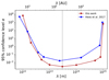 |
Fig. 2. 95% confidence level on |α| obtained in this work (red dots), compared with previous estimates by Hees et al. (2017) (blue dots). The dotted vertical line represents the minimum of the curve, in correspondence to λ ∼ 3 ⋅ 1013 m ∼ 200 AU. |
If we assume that the gravitational interaction is mediated by a massive boson as in massive gravity theories (where α = 1), the length scale λ corresponds to the Compton wavelength of the particle; hence, an upper limit on the graviton’s mass can be derived. Since α = 1 is excluded at 95% confidence level for λ ≲ 8 ⋅ 1014 m, this lower bound on the wavelength, λ, can be translated into an upper limit on the graviton mass, corresponding to mg ≲ 2.5 ⋅ 10−22 eV.
In the regime where λ ∼ rs2, when no 1PN acceleration is included, the presence of the Yukawa term in the equation of motion induces a prograde precession comparable to the Schwarzschild one. This is shown in Figure 1 for λ = 1013 m, where we can see that the posterior distribution P(α|D) is a Gaussian with mean around α ∼ 0.0026, as opposed to the 1PN posterior.
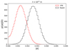 |
Fig. 1. Comparison of the posterior distributions P(|α||D) between the Keplerian model (black curve) and the 1PN model (red curve). |
Following Adkins & McDonnell (2007), we can compute the precession angle induced by a potential in a full orbit as
 (8)
(8)
where U(z) is the perturbing potential evaluated at radius r = L/(1 + ez) with L = asma(1 − e2). For α = 0.0026, this corresponds to Δϕp ∼ 0.13°. Taking the most up-to-date value of the Schwarzschild precession reported in GRAVITY Collaboration (2024), ΔϕSch = 12.1′×(0.911 ± 0.13) = (0.18 ± 0.03)°, we can see that the precession angle induced by the Yukawa potential is compatible, within the 2σ uncertainties, with ΔϕSch.
3.4. Comparison with theoretical estimates
As stated in the previous section, the inclusion of the 1PN acceleration in the equations of motion implies an additional assumption; namely, that any correction to the GR expression is subleading with respect to Eq. (3) and, hence, negligible in our fit. To show this, we compared our results obtained using Eq. (3) with the analytical expressions derived in the literature for some specific theories.
Alves et al. (2024) derived the 1PN acceleration in massive Brans-Dicke theory, which results in exactly the same expression as Eq. (3), as long as we identify α = a1/2, where a1 = 2φ/(2ω0 + 3), and set the reduced mass to η = 0, which is clearly a good approximation for the SgrA*-S2 system.
In Tan & Lu (2024) an analytical expression for the 1PN acceleration in f(R) gravity is obtained and reported in their Eq. (17). We used this expression to show that our upper limits on α are not affected by this difference in the 1PN expansion, at least when the uncertainty on α is the smallest (i.e., for λ = 3 ⋅ 1013 m). In Fig. 3, the comparison between the posteriors is reported, showing that the upper limit on α is only changed by a factor of 2 when the full expression for f(R) gravity is used.
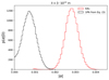 |
Fig. 3. Posterior probability density of |α| using the 1PN expression in Eq. (3) (black curve) versus the 1PN expansion for f(R) gravity derived in Tan & Lu (2024) (red curve), when λ = 3 ⋅ 1013 m. |
Tan & Lu (2024) also showed that the use of a multiple-star fit (specifically including S2, S29, and S55) with the 1PN acceleration for f(R) gravity derived in Eq. (17) could potentially break the degeneracy between M and α in the large λ limit. This could produce a stringent upper limit on the fifth force intensity for λ > 1015 m as well.
In addition, Losada et al. (2025) demonstrated that combining S2 motion with S62 lensing observations can also potentially break the degeneracy between the parametrized PN parameters β and γ. However, we leave a multi-star analysis for a future work.
4. Conclusions
In this paper, we update the current constraints on the fifth force intensity at the GC using GRAVITY data for S2 from 2017 to 2022, including the pericenter passage. These data have allowed us to significantly improve previous estimates on the same effect, giving a 95% confidence level curve that is one order of magnitude below the previous estimates (see Figure 2). Specifically, three different behaviors are found in the posterior distribution of α, according to the value of the length scale of the new interaction λ compared to S2 orbital range.
The minimum value of α is found for λ = 3 ⋅ 1013 m (∼ 200 AU) where |α|< 0.003. For comparison, in correspondence with the minimum found by Hees et al. (2017), λ = 150 AU ∼ 2.2 ⋅ 1013 m, we found |α|< 0.0031. We also showed that the 1PN expansion used in this work coincides with the expression developed for massive Brans-Dicke theory and that additional terms proportional to α in the 1PN acceleration for f(R) theories are subdominant with respect to the expression used in this work and thereby negligible, as the upper limit on |α| is unaffected.
A complete analysis including all S-stars, specifically those with apocenter passage farther away than S2, is left for future work, with the aim of further improving the confidence level curve. This would allow us to possibly expand the range of λ and obtain additional and meaningful constraints at λ ≳ 8 ⋅ 1014 m.
Acknowledgments
A.F. and F.V. would like to thank Aurélien Hees and Laura Bernard for useful comments and fruitful discussions during the preparation of this work. We are very grateful to our funding agencies (MPG, ERC, CNRS [PNCG, PNGRAM], DFG, BMBF, Paris Observatory [CS, PhyFOG], Observatoire des Sciences de l’Univers de Grenoble, and the Fundação para a Ciência e a Tecnologia), to ESO and the Paranal staff, and to the many scientific and technical staff members in our institutions, who helped to make NACO, SINFONI, and GRAVITY a reality. This project has received funding from the European Union’s Horizon 2020 research and innovation programme under the Marie Sklodowska-Curie grant agreement No 101007855. We acknowledge the financial support provided by FCT/Portugal through grants 2022.01324.PTDC, PTDC/FIS-AST/7002/2020, UIDB/00099/2020 and UIDB/04459/2020. J.S. acknowledge the National Science Foundation of China (12233001) and the National Key R&D Program of China (2022YFF0503401).
References
- Adkins, G. S., & McDonnell, J. 2007, Phys. Rev. D, 75, 082001 [Google Scholar]
- Alsing, J., Berti, E., Will, C. M., & Zaglauer, H. 2012, Phys. Rev. D, 85, 064041 [Google Scholar]
- Alves, M. F. S., Toniato, J. D., & Rodrigues, D. C. 2024, Phys. Rev. D, 109, 044045 [Google Scholar]
- Bars, I., & Visser, M. 1986, Phys. Rev. Lett., 57, 25 [Google Scholar]
- Bergé, J. 2017, in 52nd Rencontres de Moriond on Gravitation 191 [Google Scholar]
- Borka, D., Jovanović, P., Jovanović, V. B., & Zakharov, A. F. 2013, JCAP, 11, 050 [CrossRef] [Google Scholar]
- Borka, D., Jovanović, V. B., Capozziello, S., Zakharov, A. F., & Jovanović, P. 2021, Universe, 7, 407 [NASA ADS] [CrossRef] [Google Scholar]
- Capozziello, S., Borka, D., Jovanović, P., & Jovanović, V. B. 2014, Phys. Rev. D, 90, 044052 [NASA ADS] [CrossRef] [Google Scholar]
- Capozziello, S., Harko, T., Koivisto, T. S., Lobo, F. S. N., & Olmo, G. J. 2015, Universe, 1, 199 [Google Scholar]
- Carroll, S. M., Mantry, S., Ramsey-Musolf, M. J., & Stubbs, C. W. 2009, Phys. Rev. Lett., 103, 011301 [Google Scholar]
- Catanzarite, J. H. 2010, arXiv e-prints [arXiv:1008.3416] [Google Scholar]
- de Laurentis, M., De Martino, I., & Della Monica, R. 2023, Rept. Prog. Phys., 86, 104901 [Google Scholar]
- de Martino, I., della Monica, R., & de Laurentis, M., 2021, Phys. Rev. D, 104, L101502 [NASA ADS] [CrossRef] [Google Scholar]
- Della Monica, R., de Martino, I., & de Laurentis, M. 2022, MNRAS, 510, 4757 [NASA ADS] [CrossRef] [Google Scholar]
- Eckart, A., & Genzel, R. 1996, Nature, 383, 415 [NASA ADS] [CrossRef] [Google Scholar]
- Esposito, G. 2011, arXiv e-prints [arXiv:1108.3269] [Google Scholar]
- Fienga, A., & Minazzoli, O. 2024, Living Rev. Rel., 27, 1 [Google Scholar]
- Foreman-Mackey, D., Hogg, D. W., Lang, D., & Goodman, J. 2013, PASP, 125, 306 [Google Scholar]
- Frieman, J. A., & Gradwohl, B.-A. 1991, Phys. Rev. Lett., 67, 2926 [Google Scholar]
- Ghez, A. M., Duchêne, G., Matthews, K., et al. 2003, ApJ, 586, L127 [Google Scholar]
- Gillessen, S., Eisenhauer, F., Trippe, S., et al. 2009a, ApJ, 692, 1075 [NASA ADS] [CrossRef] [Google Scholar]
- Gillessen, S., Eisenhauer, F., Fritz, T. K., et al. 2009b, ApJ, 707, L114 [Google Scholar]
- Gradwohl, B.-A., & Frieman, J. A. 1992, ApJ, 398, 407 [Google Scholar]
- GRAVITY Collaboration (Abuter, R., et al.) 2018, A&A, 615, L15 [NASA ADS] [CrossRef] [EDP Sciences] [Google Scholar]
- GRAVITY Collaboration (Abuter, R., et al.) 2020, A&A, 636, L5 [NASA ADS] [CrossRef] [EDP Sciences] [Google Scholar]
- GRAVITY Collaboration (Abuter, R., et al.) 2022, A&A, 657, L12 [NASA ADS] [CrossRef] [Google Scholar]
- GRAVITY Collaboration (Abd El Dayem, K., et al.) 2024, A&A, 692, A242 [NASA ADS] [CrossRef] [EDP Sciences] [Google Scholar]
- Grould, M., Vincent, F. H., Paumard, T., & Perrin, G. 2017, A&A, 608, A60 [NASA ADS] [CrossRef] [EDP Sciences] [Google Scholar]
- Hees, A., Do, T., Ghez, A. M., et al. 2017, Phys. Rev. Lett., 118, 211101 [Google Scholar]
- Hees, A., Folkner, W. M., Jacobson, R. A., & Park, R. S. 2014, Phys. Rev. D, 89, 102002 [Google Scholar]
- Hinterbichler, K. 2012, Rev. Mod. Phys., 84, 671 [Google Scholar]
- Hofmann, F., & Müller, J. 2018, Class. Quant. Grav., 35, 035015 [Google Scholar]
- Hoyle, C. D., Schmidt, U., Heckel, B. R., et al. 2001, Phys. Rev. Lett., 86, 1418 [Google Scholar]
- Iorio, L. 2024, General Post-Newtonian Orbital Effects: From Earth’s Satellites to the Galactic Centre (Cambridge University Press) [CrossRef] [Google Scholar]
- Jovanović, P., Borka, D., Borka Jovanović, V., & Zakharov, A. F. 2021, Eur. Phys. J. D, 75, 145 [Google Scholar]
- Jovanović, P., Jovanović, V. B., Borka, D., & Zakharov, A. F. 2023, JCAP, 03, 056 [Google Scholar]
- Jovanović, P., Jovanović, V. B., Borka, D., & Zakharov, A. F. 2024a, Phys. Rev. D, 109, 064046 [Google Scholar]
- Jovanović, P., Borka Jovanović, V., Borka, D., & Zakharov, A. F. 2024b, Symmetry, 16, 397 [Google Scholar]
- Kiefer, C. 2023, arXiv e-prints [arXiv:2302.13047] [Google Scholar]
- Konopliv, A. S., Asmar, S. W., Folkner, W. M., et al. 2011, Icarus, 211, 401 [NASA ADS] [CrossRef] [Google Scholar]
- Losada, V. d. M., Della Monica, R., de Martino, I., & De Laurentis, M. 2025, A&A, 694, A280 [NASA ADS] [CrossRef] [EDP Sciences] [Google Scholar]
- Mariani, V., Fienga, A., Minazzoli, O., Gastineau, M., & Laskar, J. 2023, Phys. Rev. D, 108, 024047 [NASA ADS] [CrossRef] [Google Scholar]
- Massey, R., Kitching, T., & Richard, J. 2010, Rept. Prog. Phys., 73, 086901 [Google Scholar]
- Moffat, J. W. 2006, JCAP, 03, 004 [NASA ADS] [CrossRef] [Google Scholar]
- Nitz, A. H., Capano, C. D., Kumar, S., et al. 2021, ApJ, 922, 76 [Google Scholar]
- Peebles, P. J. E., & Ratra, B. 2003, Rev. Mod. Phys., 75, 559 [NASA ADS] [CrossRef] [Google Scholar]
- Perivolaropoulos, L. 2010, Phys. Rev. D, 81, 047501 [Google Scholar]
- Plewa, P. M., Gillessen, S., Eisenhauer, F., et al. 2015, MNRAS, 453, 3234 [Google Scholar]
- Poisson, E., & Will, C. 2012, Gravity: Newtonian, Post-Newtonian, Relativistic (Cambridge: Cambridge University Press), 1 [Google Scholar]
- Reid, M. J., & Brunthaler, A. 2020, ApJ, 892, 39 [Google Scholar]
- Sabha, N., et al. 2012, A&A, 545, A70 [NASA ADS] [CrossRef] [EDP Sciences] [Google Scholar]
- Salucci, P. 2019, Astron. Astrophys. Rev., 27, 2 [Google Scholar]
- Schödel, R., Ott, T., Genzel, R., et al. 2002, Nature, 419, 694 [Google Scholar]
- Shankaranarayanan, S., & Johnson, J. P. 2022, Gen. Relativ. Gravitation, 54, 44 [Google Scholar]
- Tan, Y., & Lu, Y. 2024, Phys. Rev. D, 109, 044047 [Google Scholar]
- Touboul, P., et al. 2022, Phys. Rev. Lett., 129, 121102 [CrossRef] [PubMed] [Google Scholar]
- Tsai, Y.-D., Wu, Y., Vagnozzi, S., & Visinelli, L. 2023, JCAP, 04, 031 [Google Scholar]
- Tsai, Y.-D., Farnocchia, D., Micheli, M., Vagnozzi, S., & Visinelli, L. 2024, Commun. Phys., 7, 311 [Google Scholar]
- Vagnozzi, S., et al. 2023, Class. Quant. Grav., 40, 165007 [NASA ADS] [CrossRef] [Google Scholar]
- van Albada, T. S., Bahcall, J. N., Begeman, K., & Sancisi, R. 1985, ApJ, 295, 305 [Google Scholar]
- Visser, M. 1998, Gen. Rel. Grav., 30, 1717 [Google Scholar]
- Weinberg, S. 1989, Rev. Mod. Phys., 61, 1 [NASA ADS] [CrossRef] [Google Scholar]
- Will, C. M. 2014, Living Rev. Rel., 17, 4 [Google Scholar]
- Will, C. M. 2018a, Theory and Experiment in Gravitational Physics (Cambridge University Press) [CrossRef] [Google Scholar]
- Will, C. M. 2018b, Class. Quant. Grav., 35, 17LT01 [Google Scholar]
- Zakharov, A. F., Jovanovic, P., Borka, D., & Jovanovic, V. B. 2016, JCAP, 05, 045 [CrossRef] [Google Scholar]
- Zakharov, A. F., Jovanović, P., Borka, D., & Borka Jovanović, V. 2018, JCAP, 04, 050 [Google Scholar]
Appendix A: Details of the numerical integration
The numerical integration of the equation of motion is performed using the Python library scipy.integrate.solve_ivp with a Runge-Kutta 5(4) algorithm, which means that the steps are evaluated using a fifth-order method, while the error is controlled assuming the accuracy of the fourth-order method. The convergence of the integration is ensured by looking at the conservation of energy over the entire integration period (almost two orbits in ∼30 years gives ΔE/E ∼ 𝒪(10−10)).
Kepler’s equation can be solved instead using a Python root finder (scipy.optimize.newton), which implements the Newton-Raphson method. The latter solves the equation with a precision of 𝒪(10−16).
Appendix B: Coordinates transformations and inclusion of relativistic effects.
B.1. Coordinate transformation
The transformation from the orbital reference frame to the observer reference frame can be achieved by using the following conversion:
 (B.1)
(B.1)
where A, B, C, F, G, H are the Thiele-Innes parameters (Catanzarite 2010) defined as:
 (B.2)
(B.2)
The Cartesian coordinates {xBH, yBH, zBH} and velocities {vxBH, vyBH, vzBH} are those obtained from the numerical integration. For a more detailed discussion on how the coordinate system {x′,y′,zobs} and the above transformation are defined, we refer to Figure 1 and Appendix B of Grould et al. (2017).
B.2. Relativistic effects and Rømer’s delay
To produce a better fit, there are observational effects that must be included in the model.
Rømer’s delay is the difference between the time of emission of the signal tem and the actual observational dates tobs, due to the finite speed of light. To include this delay, we used the first order Taylor’s expansion of the Røemer equation, which is expressed as:
 (B.3)
(B.3)
The difference between the exact solution of Røemer equation and the approximated solution in (B.3) is at most ∼4 s over the S2 orbit and therefore negligible. The Rømer effect affects both the astrometry and the spectroscopy, with an impact of ≈450 μas on positions and ≈50 km/s at periastron on radial velocities. Our results recover the previous estimates for this effect reported in Grould et al. (2017), GRAVITY Collaboration (2018).
Moreover, there are two relativistic effects that must be taken into account when S2 approaches the periastron: the relativistic Doppler shift and the gravitational redshift. Both induce a shift in the spectral lines of S2 that affects the radial velocity measurements. The former is given by
 (B.4)
(B.4)
while the gravitational redshift is defined as
 (B.5)
(B.5)
where U(rem) is the potential in Eq. (1) evaluated at the time of emission tem.
The two shifts can be combined using Eq. (D.13) of Grould et al. (2017) to obtain the total radial velocity
 (B.6)
(B.6)
where ϵ = 2U(rem).
In the total space velocity, v = |v|, we must also add a correction due to Solar System motion. We followed the most recent work of Reid & Brunthaler (2020) and take a proper motion of Sgr A* of
 (B.7)
(B.7)
All Tables
All Figures
|
Fig. 2. 95% confidence level on |α| obtained in this work (red dots), compared with previous estimates by Hees et al. (2017) (blue dots). The dotted vertical line represents the minimum of the curve, in correspondence to λ ∼ 3 ⋅ 1013 m ∼ 200 AU. |
| In the text | |
|
Fig. 1. Comparison of the posterior distributions P(|α||D) between the Keplerian model (black curve) and the 1PN model (red curve). |
| In the text | |
|
Fig. 3. Posterior probability density of |α| using the 1PN expression in Eq. (3) (black curve) versus the 1PN expansion for f(R) gravity derived in Tan & Lu (2024) (red curve), when λ = 3 ⋅ 1013 m. |
| In the text | |
Current usage metrics show cumulative count of Article Views (full-text article views including HTML views, PDF and ePub downloads, according to the available data) and Abstracts Views on Vision4Press platform.
Data correspond to usage on the plateform after 2015. The current usage metrics is available 48-96 hours after online publication and is updated daily on week days.
Initial download of the metrics may take a while.