| Issue |
A&A
Volume 692, December 2024
|
|
|---|---|---|
| Article Number | A261 | |
| Number of page(s) | 9 | |
| Section | Interstellar and circumstellar matter | |
| DOI | https://doi.org/10.1051/0004-6361/202451858 | |
| Published online | 18 December 2024 | |
Effects of the grain temperature distribution on the organic chemistry of protostellar envelopes
Engineering Research Institute ‘Ventspils International Radio Astronomy Centre’ of Ventspils University of Applied Sciences,
Inženieru 101,
Ventspils,
LV-3601,
Latvia
★ Corresponding author; This email address is being protected from spambots. You need JavaScript enabled to view it.
Received:
11
August
2024
Accepted:
18
November
2024
Abstract
Context. Dust grains in circumstellar envelopes are likely to have a spread-out temperature distribution.
Aims. We investigate how trends in the temperature distribution between small and large grains affect the hot-corino chemistry of complex organic molecules (COMs) and warm carbon-chain chemistry (WCCC).
Methods. A multi-grain multi-layer astrochemical code with an advanced treatment of the surface chemistry was used with three grain-temperature trends: a grain temperature proportional to the grain radius to the power -1/6 (Model M-1/6), to 0 (M0), and to 1/6 (M1/6). The cases of hot-corino chemistry and WCCC were investigated for a total of six models. The essence of these changes is that the main ice reservoir (small grains) has a higher (M-1/6) or lower (M1/6) temperature than the surrounding gas.
Results. The chemistry of COMs agrees better with observations in models M-1/6 and M1/6 than in Model M0. Model M-1/6 agrees best for WCCC because earlier mass-evaporation of methane ice from small grains induces the WCCC phenomenon at lower temperatures.
Conclusions. Models considering several grain populations with different temperatures reproduce the circumstellar chemistry more precisely.
Key words: astrochemistry / molecular processes / methods: numerical / stars: formation / ISM: clouds / dust, extinction
© The Authors 2024
 Open Access article, published by EDP Sciences, under the terms of the Creative Commons Attribution License (https://creativecommons.org/licenses/by/4.0), which permits unrestricted use, distribution, and reproduction in any medium, provided the original work is properly cited.
This article is published in open access under the Subscribe to Open model. This email address is being protected from spambots. You need JavaScript enabled to view it. to support open access publication.
1 Introduction
The chemical modelling of the interstellar medium, star-forming regions, and protoplanetary disks has revealed the importance of differences in the dust temperature Td between small and large grains. For grains with a size (radius) a of about some micrometers (μm) or more, the temperature decreases with larger a. For smaller grains that characterise the interstellar and circumstellar medium, studies indicated different trends. Li & Draine (2001), Cuppen et al. (2006), Krügel (2007), Röllig et al. (2013), and Iqbal & Wakelam (2018) found that small grains with a < 0.05 μm generally have the highest Td, while Heese et al. (2017), Sipilä et al. (2020), and Gavino et al. (2021) reported an opposite result, according to which large ≈0.2 μm grains have the highest Td. The sub-μm size range is dominant in a variety of astrophysical environments, such as the diffuse medium, photodissociation regions, molecular clouds, and protostellar envelopes.
We analyse the astrochemical significance of the grain-size temperature dependence problem for star-forming regions with a multi-layer astrochemical model. Instead of attempting to produce a version of the Td distribution between sub-μm grains, we investigate two main cases: First, smaller grains with a higher temperature than larger grains Td,small > Td,big, and second, Td,small < Td,big. An intermediate case with Td,small = Td,big was also considered. In a positive scenario, the comparison of our calculation results with published observations of gas and ice molecules can indicate an astrochemically preferential trend in the Td distribution between the grain sizes.
A practical goal of this study was the application and adaptation of the recently improved multi-grain multi-layer model ALCHEMIC-VENTA for describing evaporating ices. This is a necessary capability for further research. As far as we know, astrochemical models considering multiple grain types have not yet been applied for the case of evaporating ices in protostellar envelopes.
2 Methods
In our recent work, (Kalvāns et al. 2024, hereinafter KKV24) we developed a rate-equation astrochemical model with a detailed description of the gas-grain chemistry. It combines multi-sized grains and multi-layered ices, where the desorption (or surface binding) energy ED of icy molecules partially depends on their surrounding environment, whether this is bare grains, polar icy species, or non-polar ices. In addition to evaporation and surface diffusion, other important ED-dependent processes added were desorption by the exothermic H+H surface reaction, photodesorption, and chemical desorption. We found that multiple types of ED-dependent desorption mechanisms shape the formation of interstellar ices. The gas-grain chemical balance is changed by a rapid chemical desorption and a fast adsorption due to a higher surface area with the multi-grain approach.
The multi-grain multi-layer approach of KKV24 focussed on microscopic surface processes, and thus, the model is well adapted for the aims of this study. A brief explanation of the model features is provided below. Because the model is the same as in KKV24, we keep the description concise, and we focus on the few changes we introduced for the purposes of this study.
Desorption-related updates to surface species: List of species added to the H-bond rule, with ED reduced by 500 K on completely bare grains.
2.1 Chemical model
We employed the UMIST RATE2012 gas-phase network of McElroy et al. (2013) combined with the OSU surface chemistry network of Garrod et al. (2008). The latter was reduced to account only for species included in RATE2012. The initial chemical abundances are listed in Table 1 of KKV24 and were adapted from Wakelam & Herbst (2008) and Garrod (2013).
Neutral gas-phase species are accreted onto the grains, where they are sequentially arranged in three bulk-ice layers and a surface layer. Surface and bulk-ice species are subjected to photodissociation (modified by a factor of 0.3, relative to the gas-phase species) and binary reactions. For the latter, the ratio of ED and the surface diffusion energy Ediff was taken to be 0.5. The activation energy barriers EA for the CO2-generating surface reactions CO + O and CO + OH important for ice chemistry are 630 K and 176 K, respectively.
The value of ED for each molecule varies depending on the surroundings (bare grain, H2O-, or CO-dominated ices) in each layer and each grain-size bin (Sects. 2.4 and 2.5 of KKV24). On bare-grain carbonaceous surfaces, hydrogen bonds are unable to form, and the molecular ED is therefore reduced according to the H-bond rule described with Table 5 of KKV24. We extended the H-bond rule for strongly polar species with a dipole moment in excess of 2D that has no H atom attached to an electronegative atom or functional group, as listed in Table 1. The value of ED on completely bare grains was reduced by 500 K for these species compared to ED on a water surface. This change reflects the ability of these species to contribute an electron pair for a H-bond in a watery environment and the inability to do this on a carbonaceous or silicate surface.
The core is irradiated by interstellar photons (Habing field), attenuated by interstellar extinction AV, and cosmic rays (CRs), attenuated by the column of matter between the margin of the cloud and its centre. The hydrogen atom column density NH = 2.2 × 10²¹ AV cm−2.
The model considers six mechanisms for surface molecule desorption: thermal evaporation, photodesorption by interstellar and CR-induced photons, CR-induced whole-grain heating, chemical desorption of products in exothermic surface reactions, and indirect chemical desorption by a H+H combination reaction on the grains. Following the conclusions of Sipilä et al. (2019) and KKV24, we reduced the chemical desorption efficiency fcd from icy surfaces (i.e. excluding bare grains) by a factor of 0.1 for reactions producing hydrogen nitrides.
2.2 Temperature model
Five grain-size bins were considered that covered a size range of 0.03 to 0.3 μm. The bins were logarithmically distributed with the Mathis-Rumpl-Nordsieck (Mathis et al. 1977) interstellar grain-size distribution. The radius of the smallest grains is a = 0.037 μm, and that of the largest grains is 0.232 μm (Table 3 of KKV24).
In the prestellar stage, the gas temperature Tgas and Td were calculated as functions of AV based on the star-forming region simulation results by Hocuk et al. (2016) and Hocuk et al. (2017), respectively. The latter study provides the temperature Td,0.1 for a classical grain radius of 0.1 μm. This value was then used to obtain Td for the grain sizes that we used in the simulations.
As discussed in Sect. 1, several complex temperature calculations for small and large grains show opposite trends. For our aims, we adopted the simple grain size-temperature dependence of Krügel (2007), where Td ∝ ay, where the power 0 ≤ y <1
![Mathematical equation: $\[T_{d, a}=\left(\frac{a+b}{0.1}\right)^{y} \times T_{d, 0.1}.\]$](/articles/aa/full_html/2024/12/aa51858-24/aa51858-24-eq1.png) (1)
(1)
Here, b is the ice thickness (μm), with a+b being the full radius of a grain. For the trend in which the small grains have a higher Td, we took y=−1/6 (Model ‘M-1/6’, Krügel 2007; Pauly & Garrod 2016). For the opposite trend, we simply employed Td ∝ a1/6 (y=1/6; Model M1/6). Li & Draine (2001) and Heese et al. (2017) indicated a fainter Td dependence on the grain radius and likely −1/6 < y < 1/6. Therefore, with Model M0, we considered a case in which all grains have equal Td. These models were further divided into two versions that were adapted for different groups of organic compounds (Sect. 2.3). The model information is summarised in Table 2.
Positive y is supported by a simple test calculation of the dust temperature around a low-mass protostar, which was made for this study with the RADMC-3D program1 (e.g., Commerçon et al. 2012). The protostar was assumed to have a 4700 K surface temperature and a luminosity of 3 L⊙. The grain temperature varies with the distance from the star (i.e. the amount of electromagnetic radiation energy received) and a. Figure 1 shows that a factor that is even more important than size is the grain material, of which two types of amorphous interstellar silicate were considered: MgFeSiO4 and Mg2SiO4. With this method, y < 0.1, or a difference Td,0.232 − Td,0.037 of <10 K between the largest 0.232 μm and smallest 0.037 μm grains when Td,0.1 ≈ 100 K. When we differentiate grain populations by their materials and not by their sizes, the Td difference for grains of similar sizes and different materials, Td,MgFeSiO4 − Td,Mg2SiO4, is significantly greater at ≈70 K. This result is a strong indication that notable Td differences between circumstellar grain populations exist at the same time and place. We retained the Td dependence on a to continue the work in KKV24, although a Td dependence on the grain materials can be relatively straightforwardly implemented.
The temperatures in the protostellar stage were anchored at Td,0.1. As described in Sect. 2.3, Td,0.1 rises from <10 K at the end of the prestellar stage to 200 K at the protostellar envelope stage. Td for the five grain-size bins was calculated from Td,0.1 with the help of Eq. (1), except for Model M0, where Td = Td,0.1 for all bins.
The gas temperature changes in relation to Td in circumstellar environments (Chapillon et al. 2008; Podolak et al. 2011; Gavino et al. 2021). To study the chemical effects of different Td trends, we needed a simple approach for Tgas that does not complicate the interpretation of the gas-grain chemistry. Therefore, we assumed that Tgas = Td,0.1 in all models. This approach is in line with the above studies that showed that Tgas is similar to the Td of sub-micron grains.
Models with a different Td dependence on the grain size and physical conditions in the prestellar stage.
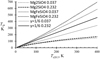 |
Fig. 1 Grain temperature difference for four types of silicate grains as a function of their average Td,0.1. The numbers in the legend indicate the size in μm. For comparison, the only-size-dependent Td employed by our model is also shown, with exponent y=1/6. (The case with y=−1/6 is almost identical, with the large- and small-grain lines swapping places.) The value of Td,0.1 on the x-axis practically depends on the amount of radiation received (or, therefore, on the distance) from the protostar. |
2.3 Macrophysical model
The model applies a standard approach for modelling an interstellar molecular star-forming cloud core. A parcel of matter near the centre of a low-mass 2 M⊙ core was considered with an initial AV=0.5 mag and a hydrogen atom number density nH=2000 cm−3. The core underwent a free-fall collapse to a final density nfin, depending on the model (see below). We assumed that at this point, the protostar has formed and the density increase stops. The core has transformed into a protostellar envelope and the gas parcel is heated according to the T2 time-dependence of Garrod & Herbst (2006, i.e., ![Mathematical equation: $\[T_{d, 0.1} \propto t_{\mathrm{pr}}^{2}\]$](/articles/aa/full_html/2024/12/aa51858-24/aa51858-24-eq2.png) , where tpr is time after birth of the protostar). It reaches Tgas of 200 K over 1 Myr after the formation of the protostar. While Garrod & Herbst (2006) also included shorter heating timescales, only the long 1 Myr timescale was considered here in order to allow us to discern the gas-mediated movement of molecules between the five grain-size bins. The evaporation from multiple grain types with shorter heating timescales is investigated in another recently submitted study.
, where tpr is time after birth of the protostar). It reaches Tgas of 200 K over 1 Myr after the formation of the protostar. While Garrod & Herbst (2006) also included shorter heating timescales, only the long 1 Myr timescale was considered here in order to allow us to discern the gas-mediated movement of molecules between the five grain-size bins. The evaporation from multiple grain types with shorter heating timescales is investigated in another recently submitted study.
The above conditions are relevant for hot corinos with abundant complex organic molecules (COMs, Cazaux et al. 2003) and warm carbon-chain chemistry (WCCC) cores (Sakai et al. 2008a), which allowed us to compare the simulation results of these compounds to their observed abundances. Both groups of species are affected by the distribution trend of the grain temperatures (expressed by the variable y) in the protostellar envelope stage. These effects mostly become apparent when the gas temperature rises relatively slowly, when evaporated molecules can re-freeze again onto colder grains in a different grain-size bin. This process, along with the uneven distribution of the ice mass between the grain-size bins, produces the differences between models with different Td trends. Therefore, we employed a long timescale of 1 Myr for the heating. In effect, the model describes the isochoric heating of a gas parcel approaching the protostar from the depths of the envelope.
Hot corinos and WCCC cores differ by their physical conditions. The former have nH ≈ 107...109 cm−3 and hot temperatures of a few hundred K. The latter are characterized by lower densities of nH ≈ 106 cm−3 and lukewarm conditions, with Tgas of only several tens of K. Furthermore, WCCC is apparently caused by external irradiation of the star-forming core (Lindberg et al. 2015; Taniguchi et al. 2021), with CRs being the most important ionisation agent (Kalvāns 2021; Sun et al. 2024). Many cores are between these two extremes, showing both C-chains and COMs (e.g., Mercimek et al. 2022).
Taking the above into account, the three models M-1/6, M0, and M1/6 were divided into two versions each, one for the COM chemistry, and the other for WCCC. The COM models had nfin = 108 cm−3 and a maximum final gas temperature Tmax of 200 K, while for WCCC models, nfin = 106 cm−3 and Tmax = 100 K (Table 2). Consequently, the WCCC models reached nfin at an integration time t=1.53 Myr and the protostellar stage ended at 2.23 Myr. For the COM models, these times were 1.55 and 2.57 Myr, respectively.
Regarding irradiation, the CR ionisation rate ζ was calculated as a function of NH following Ivlev et al. (2015), model High. For the COMs model, this value of ζ was modified by a factor fCR=0.1, and for the WCCC model, we used fCR=0.3. This approach was adopted from Kalvāns (2021), who reported that CRs are the primary agent promoting WCCC activity while decreasing the abundance of COMs. Other CR phenomena, such as CR-induced photon flux or whole-grain heating, were modified proportionally to ζ. The value of ζ varied from 1.2 × 10⁻¹⁶ to 1.0 × 10⁻¹⁷ s−1 for the COM model and from 4.0 × 10⁻¹⁶ to 9.3 × 10⁻¹⁷ s−1 for the WCCC. Higher ζ for the latter model can be caused for example by exposure to unattenuated CR flux at the margins of molecular clouds or by nearby massive starforming regions (see the discussion and references in Kalvāns 2021). Figure 2 shows the basic physical conditions in the COM and WCCC models.
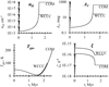 |
Fig. 2 Evolution of nH, AV, Tgas, and ζ in the COM and WCCC models. |
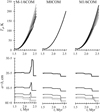 |
Fig. 3 Dust temperature and size evolution in the protostellar stage. The thicker lines show larger grains. The kinks in the Td curves above 100 K are due to the rapid change in grain size with H2O ice evaporation. |
3 Results
3.1 General chemistry
The general results of this model for the prestellar core stage depend little on the Td distribution and were discussed in detail by KKV24. Fig. 3 shows the evolution of the grain temperature and size (a+b) for the six models in the protostellar envelope stage. Grains enter the protostellar stage with an ice thickness b in the range of 66...82 monolayers (MLs), with higher b for smaller grains in all models. The abundant smallest 0.037 μm grains carry about 42% of all icy molecules at the end of the prestellar stage. The main molecular process during the heating of the envelope is evaporation of volatiles from warmer grains, accompanied by partial conversion into less volatile species and their freeze-out over long (>0.1 Myr) timescales, followed by their immediate partial re-freeze onto colder grains (in M-1/6 and M1/6) over shorter times (a few 104 yr). For the long heating timescales and high gas density considered in the COM models, the re-freeze can be nearly complete.
Overall, the gas-grain chemistry differs little between the six models. Model M-1/6COM is most similar to the model of KKV24, and we use it to describe the overall chemical results. Figure 4 shows the evolution of the abundance relative to H2 (n/n(H2)) for gaseous and solid major species in the protostellar and prestellar stages with Model M-1/6COM. A characteristic feature for this model is the see-saw pattern with four gas-phase abundance peaks for H2O and species evaporating together with H2O ice owing to successive evaporation and re-freeze from four grain-size bins when they reach Td > 100 K. Molecules that evaporated from the fifth grain-size bin have no colder grains on which to freeze-out again, and their transition to the gas phase is permanent. The saw is less pronounced in Model M1/6COM with positive y (i.e. higher Td for larger grains), because most of the ice mass is on the small grains, which evaporate last, while naturally, there are no such peaks in Model M0COM with equal Td for all grains.
The increase in the grain size due to the re-freeze in Model M-1/6COM lowers Td for grains that currently experience ice accumulation, and it makes the repeated freeze-out more efficient (see also Fig. 5). Although the gas abundance of H2O varies by three orders of magnitude in the see-saw period (2.20–2.38 Myr), it actually represents less than 0.3% of the overall H2O abundance. The amount of H2O ice (3.1 × 10⁻⁴ relative to H2), integrated over all grain sizes, practically does not change until H2O evaporation from the hottest small grains commences at 2.38 Myr and Td,0.037 = 108 K in Model M-1/6COM.
Interestingly, the re-freeze process is present even in Model MOCOM to some extent as molecules that evaporated from larger grains freeze onto smaller grains, although they all share equal Td. This phenomenon is possible because until Td < 120 K, the accretion rate onto the 0.037 μm grains is faster than thermal desorption because the surface area of the finely dispersed small grains is larger. The accretion rate is boosted by evaporation from other grain-size bins, which increases the gas-phase abundance of H2O and other species with similar ED. This temporarily shifts the accretion-evaporation balance towards freeze-out onto small grains.
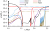 |
Fig. 4 Overall chemical results for the freeze-out period and the protostellar stage in Model M-1/6COM. We show the abundances of selected major species in gas (solid lines) and ices (dashed lines). |
3.2 COMs in the hot corino
Heavy molecules in protostellar envelopes arise in thermal desorption from ice-covered grains, with limited processing in the gas. As a means for sampling circumstellar organic synthesis in ices, gaseous COMs have raised significant interest. More than a dozen COMs are routinely detected in low-mass Class 0/I star-forming cores (Ceccarelli et al. 2023).
Thermal desorption from grains of a typical icy COM starts with its desorption from the outer surface of the hottest grain-size bin, experiences re-freeze onto colder grains, until the next grain size heats up sufficiently. Figure 5 shows that many of the COM gas-phase abundance curves show the four-peak saw from the evaporation – re-freeze cycles in Model M-1/6COM. The highest abundance achieved in these cycles is lower by at least an order of magnitude than the species abundance after its full evaporation.
These cycles end either with a species diffusion out of the bulk-ice of the coldest remaining grain-size bin that has been heated too much to sustain these species in its ice layer or with the species evaporation and non-thermal desorption from a near-bare dust surface. The latter scenario occurs after the evaporation of major species H2O, NH3, and CH3OH, when no bulk-ice remains in which the COMs can hide. Most COMs have desorption or bulk-ice diffusion energies comparable to those of water. The decrease in the H2O ice abundance by a factor of 10 occurs first for Model M0COM at t=2.35 Myr, gradually from 2.35 to 2.42 Myr for M1/6COM, and at 2.43 Myr for M-1/6 COM. This sequence is generally also obeyed by COMs. It is regulated by the inability of grains to sustain H2O ice at Td > 108 K, although evaporation of major remaining ice components begins already at 102 K. For Model M-1/6COM, the final ice-evaporation event occurs from the low number of grains in the largest size bin with a nearly 400 MLs thick ice layer. The accompanying increase in the grain size delays the programmed increase in the large-grain temperature Td,0.0232, and it even temporarily reverses it at Td,0.0232 ≈ 103 K (2.35 Myr). This effect causes an unexpected delay in the ice evaporation for Model M-1/6COM compared to M0COM and M1/6COM, where no such dramatic change in the grain size occurs. The H2O ice evaporation ends at Td ≈ 125 K, which predictably is a lower temperature than was obtained from temperature-programmed laboratory experiments with astrophysical ices (Fayolle et al. 2011; Martín-Doménech et al. 2014).
Table 3 compares the calculated gas-phase COM abundances relative to CH3OH for Models M-1/6COM, M0COM, and M1/6COM, along with observational data for the low-mass protostar IRAS 16293B that was surveyed with the Atacama Large Millimeter Array. To make maximum use of the modelled data, we applied a twofold comparison with the observations: the average abundances in the 150–200 K interval, when all ices have evaporated (t=2.43...2.57 Myr), and the final abundances at 200 K. Average abundances are useful here because the time-evolution of the model, which tracks an infalling parcel of matter, qualitatively represents the 1D chemical structure of the protostellar envelope. This effectively crudely mimicks the observational line of sight (Garrod & Herbst 2006). We adopted a difference within an order of magnitude as the basic measure for an agreement’, that is, a fit of the modelled and observed abundances. The final row of Table 3 shows that the number of these fits is highest for Model M1/6COM for the average and final abundance comparison. To evaluate this result statistically, we applied the confidence parameter κi of Garrod et al. (2007, see also Song et al. 2024),
![Mathematical equation: $\[\kappa_{i}=erfc\left(\frac{\left|\lg \left(X_{i}\right)-\lg \left(X_{\mathrm{obs}, i}\right)\right|}{\sqrt{2} \sigma}\right),\]$](/articles/aa/full_html/2024/12/aa51858-24/aa51858-24-eq3.png) (2)
(2)
where Xi is the calculated (relative) abundance of species i, Xobs,i is the observed abundance, and σ was assumed to be unity. To evaluate the modelling results, we used the ![Mathematical equation: $\[\bar{\kappa}\]$](/articles/aa/full_html/2024/12/aa51858-24/aa51858-24-eq4.png) value averaged over all entries in Table 3 and
value averaged over all entries in Table 3 and ![Mathematical equation: $\[\bar{\kappa}_{\text {red }}\]$](/articles/aa/full_html/2024/12/aa51858-24/aa51858-24-eq5.png) for a reduced number of species, namely those that observationally agreed at least for one of the models. In effect,
for a reduced number of species, namely those that observationally agreed at least for one of the models. In effect, ![Mathematical equation: $\[\bar{\kappa}_{\text {red }}\]$](/articles/aa/full_html/2024/12/aa51858-24/aa51858-24-eq6.png) excludes observed molecules with a possible contamination from regions with significantly different physical conditions and molecules with an insufficient chemical network in the model. Table 3 shows that the κ parameters are lowest for Model MOCOM in all cases, and they are generally highest for Model M1/6COM. When we draw a single average value from the four
excludes observed molecules with a possible contamination from regions with significantly different physical conditions and molecules with an insufficient chemical network in the model. Table 3 shows that the κ parameters are lowest for Model MOCOM in all cases, and they are generally highest for Model M1/6COM. When we draw a single average value from the four ![Mathematical equation: $\[\bar{\kappa}\]$](/articles/aa/full_html/2024/12/aa51858-24/aa51858-24-eq7.png) values available for each model, then the value for this ‘
values available for each model, then the value for this ‘![Mathematical equation: $\[\bar{\kappa}_{\kappa}\]$](/articles/aa/full_html/2024/12/aa51858-24/aa51858-24-eq8.png) ’ parameter is 0.351, 0.316, and 0.379 for Models M-1/6COM, M0COM, and M1/6COM, respectively.
’ parameter is 0.351, 0.316, and 0.379 for Models M-1/6COM, M0COM, and M1/6COM, respectively.
Model M0COM agrees less well with the observations, implying that a gradual evaporation of ices from grains with a spread-out Td distribution explains the observations better. The early evaporation of icy COMs (primarily CH3OH) in Model M0COM causes their over-processing in the gas, producing an overabundance of CH3OH derivatives, such as H2CO, C2H5OH, CH3OCH3, and CH3CHO. The spread in Td in Models M1/6COM and M-1/6COM mitigates the over-processing, especially by denying high CH3OH abundances at gas temperatures of 125–145 K (2.35–2.41 Myr), when CH3OH is transformed into H2CO with a high efficiency. Model M1/6COM shows the highest number of fits with observed abundances and the highest ![Mathematical equation: $\[\bar{\kappa}_{\kappa}\]$](/articles/aa/full_html/2024/12/aa51858-24/aa51858-24-eq9.png) , and this model thus agrees best with the hot-corino chemistry.
, and this model thus agrees best with the hot-corino chemistry.
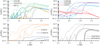 |
Fig. 5 Calculated abundances of COMs in the late protostellar stage with Tgas ≥ 90 K. The solid lines show Model M-1/6COM, the dashed lines show M0COM, and the dotted lines show M1/6COM. |
3.3 WCCC
Carbon chains can be described with a general chemical formula RCnR, where the functional groups R can either be non-existent or H, CH3, CN, S, or other atoms. Figure 6 shows the evolution of the gas-phase abundance of an example carbon chain, C7H2. Its abundance initially peaks at the prestellar stage at t ≈ 1.1 Myr, when AV ≈ 1.2 mag and nH ≈ 104 cm−3. The next peak occurs near the star formation time, when the density has rapidly increased and the irradiation level dropped, which allows different molecules to form. These peaks occur in a starless cloud and are produced by cold interstellar chemistry.
In the protostellar envelope, C7H2 reappears with an uneven abundance curve. Periods with an increasing abundance are primarily caused by evaporation of hydrocarbon ices. The evaporated species are dissociated in the gas by CR-induced photons, creating the WCCC phenomenon. It produces longer chains that promptly freeze out and again lock carbon atoms away, which ends the current gas-phase C-chain abundance bump, until the temperature rises sufficiently for the next cycle (Taniguchi et al. 2019). Because ζ is lower, the bumps are more spread out than those reported by Kalvāns (2021). The newly frozen chains reside on the outer surface of the grains, which means that CR-induced ice photoprocessing still maintains elevated gas-phase C-chain abundances between the bumps.
Unlike the hot-corino model in the above section, multiple peaks associated with the successive evaporation of the species from the five grain-size bins were not obtained for carbon chains. This was because the differences (a few K) Td between the bins were lower and the temperature rose more slowly. Evaporation from different grain-size bins and ice layers effectively overlaps, while lower nH means a lower rate for the gas molecule re-accretion onto grain surfaces. Instead, COMs evaporate at conditions of Td differences of some dozen K when the temperatures increase rapidly, which causes the sudden evaporation of volatiles, while the higher nH allows for a rapid re-freeze process that produces the four abundance peaks in Model M-1/6COM above Tgas = 100 K.
The observational conditions for WCCC are characterized by low beam-averaged temperatures of 10–15 K (Sakai et al. 2008a, 2009a) and evaporation of methane ice (Sakai et al. 2012). Thus, we attribute only the first few C-chain abundance peaks to WCCC, which occur in the t interval of 1.8–2.0 Myr and 20–50 K Tgas for all WCCC models. The elevated C-chain abundances continue up to 2.1 Myr and gas temperatures of 70 K, which we deem too high to represent the WCCC phenomenon. Figure 6 shows that the C-chain chemistry is initially reactivated in the protostellar stage after the evaporation of CO ice. This event is accompanied by a partial re-freeze of carbon and oxygen in the form of CH4 and H2O ices. The non-thermal desorption of outer-surface CH4 ice then starts low-level C-chain activity in the gas. The next major peak occurs with the thermal desorption of CH4 ice, which starts at Td > 34 K and continues with the evaporation of C2H6 ice at Td > 45 K. The peaks occur at the same t and Tgas for all C-chains in a given simulation.
Figure 7 shows example WCCC abundances for chains with the general formula RC4R. The C-chain abundance peaks shift between simulations with different grain temperature distributions. The peak due to methane evaporation occurs at t ≈ 1.92, 1.95, and 1.97 Myr for Models M-1/6WCCC, M0WCCC, and M1/6WCCC, respectively. This sequence can be explained with the temperature of the primary ice reservoir (small grain-size bins, Td,0.037) relative to that of gas. When Td,0.037 > Tgas (M-1/6), the evaporation of hydrocarbon ices occurs earlier and WCCC is observed at lower Tgas, and vice versa. The peak due to evaporation of ethane ice is only visible for some species at 2.00–2.04 Myr.
Table A.1 compares the calculated C-chain abundances with observed values. The prototypical WCCC core L1527 has the best sample of astrochemical observations and was used as a reference. To quantify the agreement with observations, we compared the average abundance in 20–50 K with the observed values. We again assumed that the evolution in time partially represents the 1D chemical make-up of the protostellar envelope. This comparison yielded indistinguishable results for all models because the average abundances usually differed within a factor of few. The values of ![Mathematical equation: $\[\bar{\kappa}\]$](/articles/aa/full_html/2024/12/aa51858-24/aa51858-24-eq12.png) and
and ![Mathematical equation: $\[\bar{\kappa}_{\text {red }}\]$](/articles/aa/full_html/2024/12/aa51858-24/aa51858-24-eq13.png) are close to 0.47 and 0.59 in all cases, respectively. The number of calculated n/n(H2) falling within a factor of 10 from observations is close to 20. A similar conclusion was reached when we used maximum instead of average abundances.
are close to 0.47 and 0.59 in all cases, respectively. The number of calculated n/n(H2) falling within a factor of 10 from observations is close to 20. A similar conclusion was reached when we used maximum instead of average abundances.
In order to further determine the differences between the M-1/6, M0, and M1/6 WCCC model results, we compared the gas temperature Tpeak of the highest abundance peak of a species in the 15–50 K interval. The observations indicate that the WCCC phenomenon occurs at low temperatures of >13 K (Sakai & Yamamoto 2013), while the C-chain abundance peaks in our models are closer to 40 K. Therefore, we assumed that lower Tpeak values indicate that a model reproduces WCCC better. The evaluation based on Tpeak clearly favours Model M-1/6WCCC because the C-chain peaks have a temperature sequence M-1/6WCCC – M0WCC – M1/6WCCC, which means that for M-1/6WCCC, the peaks consistently occur at the lowest Tgas. The latter aspect arises because the primary ice reservoir (small grains) has a higher temperature than Tgas in M-1/6WCCC and evaporates their ices earlier, at lower Tgas. These results support a negative y, where small grains have Td higher than those of large grains. This is shown quantitatively in Table A.1, where the peak abundances from a minimum Tgas of 15 K (at t=1.74 Myr) of the protostellar stage up to 50 K (t=2.01 Myr) are listed. We assume that the significant Tpeak difference between the models is 3 K because it produces a difference in magnitude of about 2 in the evaporation rate of CH4 and C2H6 ices. Compared to our previous study of WCCC (Kalvāns 2021), the C-chain abundance maxima are shifted to higher Tpeak because the ED we adopted for CH4 was higher, and thus, the evaporation temperature for CH4 ices is higher as well.
Comparison of observed (Drozdovskaya et al. 2019; Jørgensen et al. 2020) and calculated average (150–200 K) and final (200 K) gas-phase abundances relative to methanol for COMs and other species.
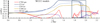 |
Fig. 6 Correlation of an example WCCC molecule C7H2 with an evaporation of C-containing ices CO, CH4, and C2 H6. The solid lines show Model M-1/6WCCC, the dashed lines show M0WCCC, and the dotted lines show M1/6WCCC. The box at t = 1.8...2.1 Myr (Tgas = 20...70 K) outlines the window with C-chain abundance peaks, which is most relevant for WCCC with this model. |
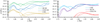 |
Fig. 7 Example calculated carbon-chain abundances in the WCCC window. The solid lines show Model M-1/6WCCC, the dashed lines show M0WCCC, and the dotted lines show M1/6WCCC. |
4 Conclusions
The comparison of calculated abundances of COMs with those observed in hot corinos showed that Models M-1/6COM and M1/6COM agree better for relative proportions between the various COMs than Model M0COM. For WCCC, the C-chain gas-phase abundance peaks in Model M-1/6WCCC occur at a lower gas temperature, which facilitates the association with the WCCC phenomenon from observations. This result is also supported by the observation of the ![Mathematical equation: $\[\mathrm{HCO}_{2}^{+}\]$](/articles/aa/full_html/2024/12/aa51858-24/aa51858-24-eq14.png) ion at a WCCC source (Sakai et al. 2009a, see also Fig. 6). The abundance of this ion rises with the desorption of CO2 ice, which also occurs at lower Tgas in Model M-1/6WCCC. In this respect, Model M1/6WCCC shows the least agreement with these observational trends, and MOWCCC is in the middle. The comparison of observed and calculated abundances yielded similar results for all three WCCC models.
ion at a WCCC source (Sakai et al. 2009a, see also Fig. 6). The abundance of this ion rises with the desorption of CO2 ice, which also occurs at lower Tgas in Model M-1/6WCCC. In this respect, Model M1/6WCCC shows the least agreement with these observational trends, and MOWCCC is in the middle. The comparison of observed and calculated abundances yielded similar results for all three WCCC models.
The chemically important difference between all models is that in M-1/6, the main ice reservoir (small grains) has a higher temperature than the gas, in M1/6 a minority of ices have Td > Tgas and most have Td < Tgas, while for M0, all ices always have Td = Tgas. The latter is physically least feasible because, given the potential diversity of dust, not all circumstellar grains can be expected to have a similar. Their temperatures differ not only because of the different sizes, but even more so because of their chemical composition (Fig. 1 in Sect. 2.2). The M0 models serve as in situ comparison of our calculation results with the simpler single-grain-type models that are commonly used in astrochemistry. We will consider grain populations that consist of different materials in a future study.
To conclude, this investigation indicates that the introduction of the multi-grain approach clearly affects the circumstellar organic chemistry. For the interstellar cloud – prestellar collapse stage, in contrast, Models M0, M-1/6, and M1/6 produce chemical results that are similar for most species. Notably, the calculated composition of interstellar ice was found to be practically equal. This underlines that the changes in protostellar organic chemistry are produced solely by differing ice evaporation patterns in the heated protostellar envelope model.
Acknowledgements
This research is funded by the Latvian Science Council grant ‘Desorption of icy molecules in the interstellar medium (DIMD)’, project No. lzp-2021/1-0076 and has made use of NASA’s Astrophysics Data System. We thank the referee for significant improvements to the presentation.
Appendix A Results of the WCCC models
Calculated average and maximum abundances with their respective Tgas during the WCCC window of 20–50 K (1.81–2.01 Myr) for carbon-chains and other species’, relative to H2.
References
- Araki, M., Takano, S., Sakai, N., et al. 2017, ApJ, 847, 51 [Google Scholar]
- Cazaux, S., Tielens, A. G. G. M., Ceccarelli, C., et al. 2003, ApJ, 593, L51 [CrossRef] [Google Scholar]
- Ceccarelli, C., Codella, C., Balucani, N., et al. 2023, in Protostars and Planets VII, eds. S. Inutsuka, Y. Aikawa, T. Muto, K. Tomida, & M. Tamura, Astronomical Society of the Pacific Conference Series, 534, 379 [NASA ADS] [Google Scholar]
- Chapillon, E., Guilloteau, S., Dutrey, A., & Piétu, V. 2008, A&A, 488, 565 [NASA ADS] [CrossRef] [EDP Sciences] [Google Scholar]
- Commerçon, B., Launhardt, R., Dullemond, C., & Henning, T. 2012, A&A, 545, A98 [NASA ADS] [CrossRef] [EDP Sciences] [Google Scholar]
- Cordiner, M. A., Charnley, S. B., Wirström, E. S., & Smith, R. G. 2012, ApJ, 744, 131 [NASA ADS] [CrossRef] [Google Scholar]
- Cuppen, H. M., Morata, O., & Herbst, E. 2006, MNRAS, 367, 1757 [Google Scholar]
- Drozdovskaya, M. N., van Dishoeck, E. F., Rubin, M., Jørgensen, J. K., & Altwegg, K. 2019, MNRAS, 490, 50 [Google Scholar]
- Fayolle, E. C., Öberg, K. I., Cuppen, H. M., Visser, R., & Linnartz, H. 2011, A&A, 529, A74 [NASA ADS] [CrossRef] [EDP Sciences] [Google Scholar]
- Garrod, R. T. 2013, ApJ, 765, 60 [Google Scholar]
- Garrod, R. T., & Herbst, E. 2006, A&A, 457, 927 [NASA ADS] [CrossRef] [EDP Sciences] [Google Scholar]
- Garrod, R. T., Wakelam, V., & Herbst, E. 2007, A&A, 467, 1103 [NASA ADS] [CrossRef] [EDP Sciences] [Google Scholar]
- Garrod, R. T., Weaver, S. L. W., & Herbst, E. 2008, ApJ, 682, 283 [NASA ADS] [CrossRef] [Google Scholar]
- Gavino, S., Dutrey, A., Wakelam, V., et al. 2021, A&A, 654, A65 [NASA ADS] [CrossRef] [EDP Sciences] [Google Scholar]
- Heese, S., Wolf, S., Dutrey, A., & Guilloteau, S. 2017, A&A, 604, A5 [NASA ADS] [CrossRef] [EDP Sciences] [Google Scholar]
- Hirota, T., Ohishi, M., & Yamamoto, S. 2009, ApJ, 699, 585 [Google Scholar]
- Hocuk, S., Cazaux, S., Spaans, M., & Caselli, P. 2016, MNRAS, 456, 2586 [Google Scholar]
- Hocuk, S., Szûcs, L., Caselli, P., et al. 2017, A&A, 604, A58 [NASA ADS] [CrossRef] [EDP Sciences] [Google Scholar]
- Iqbal, W., & Wakelam, V. 2018, A&A, 615, A20 [NASA ADS] [CrossRef] [EDP Sciences] [Google Scholar]
- Ivlev, A. V., Padovani, M., Galli, D., & Caselli, P. 2015, ApJ, 812, 135 [Google Scholar]
- Jørgensen, J. K., Schöier, F. L., & van Dishoeck, E. F. 2002, A&A, 389, 908 [CrossRef] [EDP Sciences] [Google Scholar]
- Jørgensen, J. K., Schöier, F. L., & van Dishoeck, E. F. 2004, A&A, 416, 603 [Google Scholar]
- Jørgensen, J. K., Belloche, A., & Garrod, R. T. 2020, ARA&A, 58, 727 [Google Scholar]
- Kalvāns, J. 2021, ApJ, 910, 54 [CrossRef] [Google Scholar]
- Kalvāns, J., Kalniņa, A., & Veitners, K. 2024, A&A, 687, A296 [NASA ADS] [CrossRef] [EDP Sciences] [Google Scholar]
- Krügel, E. 2007, An Introduction to the Physics of Interstellar Dust (Taylor & Francis, CRC Press) [CrossRef] [Google Scholar]
- Li, A., & Draine, B. T. 2001, ApJ, 554, 778 [Google Scholar]
- Lindberg, J. E., Jørgensen, J. K., Watanabe, Y., et al. 2015, A&A, 584, A28 [NASA ADS] [CrossRef] [EDP Sciences] [Google Scholar]
- Martín-Doménech, R., Muñoz Caro, G. M., Bueno, J., & Goesmann, F. 2014, A&A, 564, A8 [NASA ADS] [CrossRef] [EDP Sciences] [Google Scholar]
- Mathis, J. S., Rumpl, W., & Nordsieck, K. H. 1977, ApJ, 217, 425 [Google Scholar]
- McElroy, D., Walsh, C., Markwick, A. J., et al. 2013, A&A, 550, A36 [NASA ADS] [CrossRef] [EDP Sciences] [Google Scholar]
- Mercimek, S., Codella, C., Podio, L., et al. 2022, A&A, 659, A67 [NASA ADS] [CrossRef] [EDP Sciences] [Google Scholar]
- Pauly, T., & Garrod, R. T. 2016, ApJ, 817, 146 [Google Scholar]
- Podolak, M., Mayer, L., & Quinn, T. 2011, ApJ, 734, 56 [NASA ADS] [CrossRef] [Google Scholar]
- Röllig, M., Szczerba, R., Ossenkopf, V., & Glück, C. 2013, A&A, 549, A85 [Google Scholar]
- Sakai, N., & Yamamoto, S. 2013, Chem. Rev., 113, 8981 [Google Scholar]
- Sakai, N., Sakai, T., Osamura, Y., & Yamamoto, S. 2007, ApJ, 667, L65 [NASA ADS] [CrossRef] [Google Scholar]
- Sakai, N., Sakai, T., Hirota, T., & Yamamoto, S. 2008a, ApJ, 672, 371 [Google Scholar]
- Sakai, N., Sakai, T., & Yamamoto, S. 2008b, ApJ, 673, L71 [NASA ADS] [CrossRef] [Google Scholar]
- Sakai, N., Sakai, T., Hirota, T., Burton, M., & Yamamoto, S. 2009a, ApJ, 697, 769 [Google Scholar]
- Sakai, N., Sakai, T., Hirota, T., & Yamamoto, S. 2009b, ApJ, 702, 1025 [Google Scholar]
- Sakai, N., Sakai, T., Hirota, T., & Yamamoto, S. 2010, ApJ, 722, 1633 [Google Scholar]
- Sakai, N., Shirley, Y. L., Sakai, T., et al. 2012, ApJ, 758, L4 [NASA ADS] [CrossRef] [Google Scholar]
- Sipilä, O., Caselli, P., Redaelli, E., Juvela, M., & Bizzocchi, L. 2019, MNRAS, 487, 1269 [Google Scholar]
- Sipilä, O., Zhao, B., & Caselli, P. 2020, A&A, 640, A94 [NASA ADS] [CrossRef] [EDP Sciences] [Google Scholar]
- Song, Z., Chang, Q., Meng, Q., & Zhang, X. 2024, A&A, 691, A40 [NASA ADS] [CrossRef] [EDP Sciences] [Google Scholar]
- Sun, J., Li, X., Du, F., et al. 2024, A&A, 683, A76 [NASA ADS] [CrossRef] [EDP Sciences] [Google Scholar]
- Taniguchi, K., Herbst, E., Caselli, P., et al. 2019, ApJ, 881, 57 [Google Scholar]
- Taniguchi, K., Majumdar, L., Plunkett, A., et al. 2021, ApJ, 922, 152 [NASA ADS] [CrossRef] [Google Scholar]
- Wakelam, V., & Herbst, E. 2008, ApJ, 680, 371 [NASA ADS] [CrossRef] [Google Scholar]
- Yoshida, K., Sakai, N., Nishimura, Y., et al. 2019, PASJ, 71, S18 [NASA ADS] [CrossRef] [Google Scholar]
All Tables
Desorption-related updates to surface species: List of species added to the H-bond rule, with ED reduced by 500 K on completely bare grains.
Models with a different Td dependence on the grain size and physical conditions in the prestellar stage.
Comparison of observed (Drozdovskaya et al. 2019; Jørgensen et al. 2020) and calculated average (150–200 K) and final (200 K) gas-phase abundances relative to methanol for COMs and other species.
Calculated average and maximum abundances with their respective Tgas during the WCCC window of 20–50 K (1.81–2.01 Myr) for carbon-chains and other species’, relative to H2.
All Figures
|
Fig. 1 Grain temperature difference for four types of silicate grains as a function of their average Td,0.1. The numbers in the legend indicate the size in μm. For comparison, the only-size-dependent Td employed by our model is also shown, with exponent y=1/6. (The case with y=−1/6 is almost identical, with the large- and small-grain lines swapping places.) The value of Td,0.1 on the x-axis practically depends on the amount of radiation received (or, therefore, on the distance) from the protostar. |
| In the text | |
|
Fig. 2 Evolution of nH, AV, Tgas, and ζ in the COM and WCCC models. |
| In the text | |
|
Fig. 3 Dust temperature and size evolution in the protostellar stage. The thicker lines show larger grains. The kinks in the Td curves above 100 K are due to the rapid change in grain size with H2O ice evaporation. |
| In the text | |
|
Fig. 4 Overall chemical results for the freeze-out period and the protostellar stage in Model M-1/6COM. We show the abundances of selected major species in gas (solid lines) and ices (dashed lines). |
| In the text | |
|
Fig. 5 Calculated abundances of COMs in the late protostellar stage with Tgas ≥ 90 K. The solid lines show Model M-1/6COM, the dashed lines show M0COM, and the dotted lines show M1/6COM. |
| In the text | |
|
Fig. 6 Correlation of an example WCCC molecule C7H2 with an evaporation of C-containing ices CO, CH4, and C2 H6. The solid lines show Model M-1/6WCCC, the dashed lines show M0WCCC, and the dotted lines show M1/6WCCC. The box at t = 1.8...2.1 Myr (Tgas = 20...70 K) outlines the window with C-chain abundance peaks, which is most relevant for WCCC with this model. |
| In the text | |
|
Fig. 7 Example calculated carbon-chain abundances in the WCCC window. The solid lines show Model M-1/6WCCC, the dashed lines show M0WCCC, and the dotted lines show M1/6WCCC. |
| In the text | |
Current usage metrics show cumulative count of Article Views (full-text article views including HTML views, PDF and ePub downloads, according to the available data) and Abstracts Views on Vision4Press platform.
Data correspond to usage on the plateform after 2015. The current usage metrics is available 48-96 hours after online publication and is updated daily on week days.
Initial download of the metrics may take a while.