Role of diffusive and nondiffusive grain-surface processes in cold cores: Insights from the PEGASIS three-phase astrochemical model

S. Maitrey; L. Majumdar; V. Manilal; B. Srivastava; P. Rayalacheruvu; K. Willacy; E. Herbst

doi:10.1051/0004-6361/202554717

Home

All issues

Volume 699 (July 2025)

A&A, 699 (2025) A332

Full HTML

Open Access

Issue		A&A Volume 699, July 2025


Article Number		A332
Number of page(s)		20
Section		Numerical methods and codes
DOI		https://doi.org/10.1051/0004-6361/202554717
Published online		17 July 2025

A&A, 699, A332 (2025)

Role of diffusive and nondiffusive grain-surface processes in cold cores: Insights from the PEGASIS three-phase astrochemical model

S. Maitrey¹^,2^★, L. Majumdar¹^,2, V. Manilal¹^,2, B. Srivastava¹^,2, P. Rayalacheruvu¹^,2, K. Willacy³ and E. Herbst⁴

¹ Exoplanets and Planetary Formation Group, School of Earth and Planetary Sciences, National Institute of Science Education and Research, Jatni 752050, Odisha, India
² Homi Bhabha National Institute, Training School Complex, Anushaktinagar, Mumbai 400094, India
³ Jet Propulsion Laboratory, California Institute of Technology, 4800 Oak Grove Drive, Pasadena, CA 91109, USA
⁴ Department of Chemistry, University of Virginia, Charlottesville, VA 22904, USA

^★ Corresponding author: liton@niser.ac.in; dr.liton.majumdar@gmail.com

Received: 24 March 2025
Accepted: 23 April 2025

Abstract

Context. Cold, dense cores are unique among structures found in the interstellar medium, as they harbor a rich chemical inventory, including complex organic molecules (COMs), which future evolutionary stages, such as protostellar envelopes and protoplanetary disks, will inherit. These molecules exist both in the gas phase and as ices accreted onto grain surfaces.

Aims. To model these environments, we present PEGASIS: a new, fast, and extensible three-phase astrochemical code designed to explore the chemistry of cold cores, with an emphasis on the role of diffusive and nondiffusive chemistry in shaping their gas and grain chemical compositions.

Methods. We incorporate the latest developments in interstellar chemistry modeling by utilizing the 2024 Kinetic Database for Astrochemistry chemical network and comparing our results with current state-of-the-art astrochemical models. Using a traditional rate-equation-based approach, we implement both diffusive and nondiffusive chemistry, coupled with either an inert or a chemically active ice mantle.

Results. We identify crucial reactions that enhance the production of COMs through nondiffusive mechanisms on the grain surface, as well as the mechanisms through which they can accumulate in the gas phase. Across all models with nondiffusive chemistry, we observe a clear enhancement in the concentration of COMs on both the grain surface and in the grain mantle. Finally, our model broadly reproduces the observed abundances of multiple gas-phase species for the Taurus Molecular Cloud (TMC-1) and provides insights into its chemical age.

Conclusions. Our work demonstrates the capabilities of PEGASIS in exploring a wide range of grain surface chemical processes and modeling approaches for three-phase chemistry in the interstellar medium, providing robust explanations for observed abundances in cold cores, such as TMC-1 (CP). In particular, it highlights the role of nondiffusive chemistry in the production of gas-phase COMs on grain surfaces, which are subsequently chemically desorbed, especially when the precursors involved in their formation on the surfaces are heavier than atomic hydrogen.

Key words: astrochemistry / ISM: abundances / ISM: molecules

© The Authors 2025

Open Access article, published by EDP Sciences, under the terms of the Creative Commons Attribution License (https://creativecommons.org/licenses/by/4.0), which permits unrestricted use, distribution, and reproduction in any medium, provided the original work is properly cited.

This article is published in open access under the Subscribe to Open model. Subscribe to A&A to support open access publication.

1 Introduction

The accretion of gas-phase interstellar molecules on the cold dust grains plays a fundamental role in enriching the chemistry of molecular clouds. These grains facilitate several physical and chemical processes on their surfaces, which in turn lead to the formation of species that cannot be solely formed in the gas phase (see Tielens & Hagen 1982; Herbst & van Dishoeck 2009, and references therein). For example, Gould & Salpeter (1963) established that dust grains must act as catalysts to account for the presence of molecular hydrogen observed in the interstellar medium. Surface chemistry thus serves as a critical bridge, shaping both the composition of the bulk ice that forms on grains and the gas-phase composition through desorption processes. Astrochemical models capable of simulating these processes in the interstellar medium (and in various more evolved protostellar or protoplanetary environments) have existed since radio observatories became prominent in detecting interstellar molecules (Agúndez & Wakelam 2013). As the list of observed molecules continues to grow (see the Cologne Database for Molecular Spectroscopy¹ and McGuire 2022, for the most recent compilation), driven by increasingly advanced observational capabilities, it has become imperative that models also evolve. A robust astrochemical model must be able to couple gas-phase chemistry with ice chemistry while remaining versatile enough to be applied to a variety of physical environments.

For cold cores, pioneering work by Bates & Spitzer (1951); Watson (1973, 1974, 1976) and Herbst & Klemperer (1973) established key chemical processes and pathways, paving the way for the construction of chemical networks. In conjunction with experimental work, sets of reactions involving detected molecules that can occur in the interstellar medium are identified and compiled for simulation by numerical schemes. Currently, the UMIST Database for Astrochemistry (Millar et al. 1991, 1997; Le Teuff et al. 2000; Woodall et al. 2007; McElroy et al. 2013; Millar et al. 2024) and the KInetic Database for Astrochemistry (KIDA) (Wakelam et al. 2012, 2015, 2024) represent the most recent and well-maintained publicly available networks. These chemical networks typically encapsulate information about which chemical reactions and processes can proceed under specific physical conditions. These networks can then be used by various astrochemical codes for modeling. Examples of published astrochemical codes include the Willacy Model (Willacy & Millar 1998), ALCHEMIC (Semenov et al. 2010), MAGICKAL (Garrod & Pauly 2011), GRAINOBLE (Taquet et al. 2012), MONACO (Vasyunin & Herbst 2013), ASTROCHEM² (Maret et al. 2013), the Rokko code (Furuya et al. 2015), the CMMC code (Das et al. 2015), NAUTILUS³ (Ruaud et al. 2016), UCLCHEM⁴ (Holdship et al. 2017), CHEMPL⁵ (Du 2021), the Acharyya Model (Acharyya et al. 2020), and Sipilä’s Model (Sipilä et al. 2022). Several of these codes are now publicly available for broader use within the astrochemistry community as well. The approaches used by these codes to simulate chemical networks vary, but the rate equation method, which involves solving a system of coupled differential equations, has proven to be straightforward to implement and faster to converge (see Cuppen et al. 2013, for an overview on this and other techniques).

Increasingly, theoretical and laboratory studies have highlighted the importance of physicochemical processes such as photodissociation by UV radiation and cosmic rays, as well as diffusive chemistry, which extends beyond the gas phase to the grain surface and bulk mantle (Andersson & van Dishoeck 2008; Öberg et al. 2009). This makes the inclusion of an active noninert mantle crucial for evaluating the extent to which it can influence the wider gas phase chemistry. Several authors have attempted to implement this by considering each accreted ice layer individually (Taquet et al. 2012), or by grouping multiple layers as mantle phases (Furuya et al. 2017), or by extending the three-phase model of Hasegawa & Herbst (1993b) to explore effects of bulk ice chemistry (Ruaud et al. 2016; Kalvāns & Shmeld 2010; Garrod 2013).

Including ice chemistry opens up the possibility of progressive entrapment of molecules onto grains, as the gas phase reservoir depletes and both accretion and desorption rates decrease. Herbst et al. (2005) discusses the importance of nonthermal desorption pathways, especially at later ages in the lifetime of cold cores. Studies such as Garrod et al. (2006) have examined the role of desorption pathways in reproducing abundances at much later times. Essentially, considering a more detailed framework of ice chemistry and its interaction with the gas phase suggests that convergence with observations occurs increasingly at late times (see Wakelam et al. 2021, for the most recent development). Thus, the estimation of chemical ages for these sources remains uncertain.

The inner regions of dense clouds are often well shielded, allowing the bulk mantle to persist for extended periods. However, the very low temperatures in these regions (~10 K) render most heavier species immobile, making diffusion-driven production of complex organic molecules (COMs) unfeasible. This contrasts with the detection of molecules such as methyl formate (HCOOCH₃) and dimethyl ether (CH₃OCH₃) in colder regions (Cernicharo et al. 2012; Bacmann et al. 2012). Consequently, alternative pathways have been proposed to form these COMs on grain surfaces without relying on diffusive chemistry (Ruaud et al. 2015; Chang & Herbst 2016; Bergner et al. 2017a,b; Shingledecker et al. 2018; Jin & Garrod 2020), with subsequent nonthermal desorption mechanisms playing a crucial role. Notably, Balucani et al. (2015) also suggested the possibility of gas-phase formation of COMs. Jin & Garrod (2020) employed a modified-rate method introduced in Garrod (2008), demonstrating that appreciable COM production can occur even in the absence of diffusive chemistry.

As mentioned earlier, astrochemical models must be adaptable and flexible to accurately simulate chemistry across various astrochemical environments by incorporating both diffusive and nondiffusive chemistry. The inclusion of nondiffusive chemical processes is crucial for accurately modeling colder regions, whereas hotter regions require special consideration of surface chemistry. If surface molecules are assumed to be bound solely by weak van der Waals forces, the efficiency of any significant surface chemistry becomes negligible. Acharyya et al. (2020) introduced the concept of chemisorbed sites, where molecules exhibit higher binding energies, thereby enabling surface chemistry even at temperatures exceeding 100 K.

To address these challenges, we introduce PEGASIS, a fast and flexible three-phase astrochemistry code that incorporates both diffusive and nondiffusive grain-surface processes, along with all fundamental ice chemistry mechanisms applicable across diverse astrochemical environments. In this paper, we apply PEGASIS to investigate the role of both diffusive and nondiffusive grain-surface processes in shaping the gas-phase and grain-surface chemical compositions of cold cores, specifically targeting the Cyanopolyyne peak position in the Taurus Molecular Cloud (TMC-1 (CP)), given its ever-expanding and chemically rich inventory. Recent detections include several oxygen-bearing complex organic molecules-such as propenal (C₂H₃CHO), vinyl alcohol (C₂H₃OH), methyl formate (HCOOCH₃), and dimethyl ether (CH₃OCH₃) as reported by Agúndez et al. (2021), plus ethanol (CH₃CH₂OH), acetone (CH₃COCH₃), and propanal (C₂H₅CHO) reported by Agúndez et al. (2023). Additional newly identified species include 1,4-pentadiyne (HCCCH₂CCH; Fuentetaja et al. 2024), sulfur radicals (Cernicharo et al. 2024a), dinitriles (Agúndez et al. 2024), polycyclic aromatic hydrocarbons (PAHs) (Cernicharo et al. 2024b; Wenzel et al. 2024), thioacetaldehyde (CH₃CHS; Agúndez et al. 2025), the 1-cyano propargyl radical (HCCCHCN; Cabezas et al. 2025), and cyclopropenethione (c-C₃H₂S; Remijan et al. 2025).

The structure of the paper is as follows. In Section 2, we describe our model and the chemical processes it includes. Section 3 presents a benchmark comparison of PEGASIS with the public version of NAUTILUS (Ruaud et al. 2016). In Section 4, we examine the differences between the three-phase chemistry prescriptions of Ruaud et al. (2016) and Hasegawa & Herbst (1993b), and compare the predicted gas-phase abundances with observations in TMC-1 (CP), considering both diffusive and nondiffusive chemistry. Although many species have been detected in TMC-1, we restrict our discussion to those included in the 2024 KIDA chemical network. Additionally, we compare the ice abundances with those observed in more evolved sources to gain insights into the transformation of the chemical inventory from cold cores to later evolutionary stages. Finally, we summarize our conclusions in Section 5.

2 Model description

Pegasis is a three-phase model (gas, grain surface, and grain mantle) that provides a comprehensive and flexible approach to understanding how molecular abundances evolve in the interstellar medium. The code is designed to study the chemistry of molecular clouds, but it can also be easily extended to model chemistry in other evolutionary stages, such as protostars and protoplanetary disks. Following Ruaud et al. (2016), we allow chemical reactions to occur in the mantle as well as on the grain surface, albeit with a lower rate of diffusion. We implement this by setting the diffusion barrier for surface species as a smaller fraction of the binding energies (Garrod & Herbst 2006) than for mantle species. The interaction between grainsurface and gas-phase chemistry occurs through accretion and desorption processes. Desorption can occur by thermal, nonthermal, or chemical mechanisms. For the three-phase chemistry, we implement prescriptions from both Ruaud et al. (2016) and Hasegawa & Herbst (1993b). Most processes are implemented as switches, allowing their effects to be explored separately. We use the most recent release from the KIDA (Wake lam et al. 2024) as our base chemical network. This includes 7667 gas-phase reactions and 4837 grain-surface and grain-mantle reactions and processes. Pegasis is implemented entirely in Python and accelerated by Numba (Lam et al. 2024). Finally, the differential equations are solved using the DLSODES solver from the ODEPACK library (Hindmarsh 1983) wrapped as a Python extension⁶.

2.1 Modeling chemical processes

Pegasis employs a chemical kinetics-based approach to model various chemical processes, starting from a specified set of initial conditions and evolving a system of coupled differential equations over time. The initial conditions define the physical and chemical configuration of the model, together with the starting concentrations of the molecules to be considered. In the simplest scenario, only the interstellar elemental abundances are used initially. The rate coefficients for each reaction are calculated and used to determine the total production or destruction of each species in the simulation.

For each species considered, Pegasis solves a system of ordinary differential equations involving each of the chemical species that may exist in the three phases: gas, grain surface, and grain mantle. These equations describe the evolution of species abundances with time and take the form $\begin{aligned} \frac{d n_{g} (p)}{d t} |_{tot} = & \sum_{q} \sum_{r} k_{q r} n_{g} (q) n_{g} (r) \\ + k_{diss}^{g} (q) n_{g} (q) + k_{des} (p) n_{s} (p) \\ - k_{diss}^{g} (p) n_{g} (p) - k_{acc} (p) n_{g} (p) \\ - n_{g} (p) \sum_{r} k_{p q} n_{g} (q), \end{aligned}$ $\begin{split} \frac{{\rm d} n_{\text{g}}(p)}{{\rm d}t} \bigg|_{\text{tot}} = & \sum_{q} \sum_{r} k_{qr} n_{\text{g}}(q) n_{\text{g}}(r) \\ & + k^{\text{g}}_{\text{diss}}(q) n_{\text{g}}(q) + k_{\text{des}} (p) n_{\text{s}} (p) \\ & - k^{\text{g}}_{\text{diss}} (p) n_{\text{g}}(p) - k_{\text{acc}} (p) n_{\text{g}}(p) \\ & - n_{\text{g}}(p) \sum_{r} k_{pq} n_{\text{g}}(q), \end{split}$ (1) $\begin{aligned} \frac{d n_{s} (p)}{d t} |_{tot} = & \sum_{q} \sum_{r} k_{q r}^{s} n_{s} (q) n_{s} (r) \\ + k_{diss}^{s} (q) n_{s} (q) + k_{acc} (p) n_{g} (p) \\ + k_{swap}^{m} (p) n_{m} (p) + \frac{d n_{m} (p)}{d t} |_{m \to s} \\ - n_{s} (p) \sum_{q} k_{p q}^{s} n_{s} (q) \\ - k_{diss}^{s} (p) n_{s} (p) - k_{des} (p) n_{s} (p) \\ - k_{swap}^{s} (p) n_{s} (p) - \frac{d n_{s} (p)}{d t} |_{s \to m}, \end{aligned}$ $\begin{split} \frac{{\rm d} n_{\text{s}}(p)}{{\rm d}t} \bigg|_{\text{tot}} = & \sum_{q} \sum_{r} k^{\text{s}}_{qr} n_{\text{s}}(q) n_{\text{s}}(r) \\ & + k^{\text{s}}_{\text{diss}}(q) n_{\text{s}}(q) + k_{\text{acc}} (p) n_{\text{g}}(p) \\ & + k^{\text{m}}_{\text{swap}} (p) n_{\text{m}} (p) + \dfrac{{\rm d}n_{\text{m}} (p)}{{\rm d}t} \bigg|_{\text{m} \rightarrow \text{s}} \\ & - n_{\text{s}} (p) \sum_{q} k^{\text{s}}_{pq} n_{\text{s}} (q) \\ & - k^{\text{s}}_{\text{diss}} (p) n_{\text{s}} (p) - k_{\text{des}} (p) n_{\text{s}} (p) \\ & - k^{\text{s}}_{\text{swap}} (p) n_{\text{s}} (p) - \dfrac{{\rm d} n_{\text{s}} (p)}{{\rm d}t} \bigg|_{\text{s} \rightarrow \text{m}} , \end{split}$ (2) $\begin{aligned} \frac{d n_{m} (p)}{d t} |_{tot} = & \sum_{q} \sum_{r} k_{q r}^{m} n_{m} (q) n_{m} (r) \\ + k_{diss}^{m} (q) n_{m} (q) \\ + k_{swap}^{s} (p) n_{s} (p) + \frac{d n_{s} (p)}{d t} |_{s \to m} \\ - n_{m} (p) \sum_{q} k_{p q}^{m} n_{m} (q) \\ - k_{diss}^{m} (p) n_{m} (p) \\ - k_{swap}^{m} (p) n_{m} (p) - \frac{d n_{m} (p)}{d t} |_{m \to s} . \end{aligned}$ $\begin{split} \frac{{\rm d} n_{\text{m}}(p)}{{\rm d}t} \bigg|_{\text{tot}} = & \sum_{q} \sum_{r} k^{\text{m}}_{qr} n_{\text{m}}(q) n_{\text{m}}(r) \\ & + k^{\text{m}}_{\text{diss}}(q) n_{\text{m}}(q) \\ & + k^{\text{s}}_{\text{swap}} (p) n_{\text{s}} (p) + \dfrac{{\rm d}n_{\text{s}} (p)}{{\rm d}t} \bigg|_{\text{s} \rightarrow \text{m}} \\ & - n_{\text{m}} (p) \sum_{q} k^{\text{m}}_{pq} n_{\text{m}} (q) \\ & - k^{\text{m}}_{\text{diss}} (p) n_{\text{m}} (p) \\ & - k^{\text{m}}_{\text{swap}} (p) n_{\text{m}} (p) - \dfrac{{\rm d} n_{\text{m}} (p)}{{\rm d}t} \bigg|_{\text{m} \rightarrow \text{s}}. \end{split}$ (3)

Here k_pq, $k_{p q}^{s}$ $k^{\text{s}}_{pq}$ , and $k_{p q}^{m}$ $k^{\text{m}}_{pq}$ are the rate coefficients in the gas phase, grain surface, and grain mantle, respectively, between species p and q. The rate for photodissociation processes in the gas phase, surface (s), and mantle (m) phases is given by k_diss. Freeze-out (k_acc) of gaseous molecules onto the surface, and desorption (k_des) of surface species back into the gas phase, are also included. The transfer of material from the surface to the mantle and vice versa is included with rates $k_{swap}^{s}$ $k^s_{\text{swap}}$ and $k_{swap}^{m}$ $k^m_{\text{swap}}$ , respectively. It is important to note that this swapping does not represent the actual movement of material across ice layers (Hasegawa & Herbst 1993b; Garrod & Pauly 2011; Ruaud et al. 2016).

For the reactions involving two reactants (bimolecular reactions), the rate coefficient is calculated using the modified Arrhenius formula (Kooij 1893): $k = α {(T / 300)}^{β} \exp (- γ / T) .$ $k = \alpha {(T / 300)}^{\beta} \exp (-\gamma / T).$ (4)

For bimolecular reactions involving charged species, we follow Wakelam et al. (2012) and implement the temperature-dependent modification of the rate coefficients using the Su-Chesnavich capture approach discussed in Woon & Herbst (2009). Further details on the types of bimolecular reactions included in the network can be found in Wakelam et al. (2012, 2024) and references therein.

The charged gas-phase species can also react with negatively charged dust grains in a neutralization reaction, with a rate coefficient given by $k = α {(\frac{T}{300})}^{β} .$ $k = \alpha {\left(\dfrac{T}{300}\right)}^{\beta}.$ (5)

Here, the activation energy γ is set to zero, as this type of recombination reaction is considered barrierless (Geppert & Larsson 2008). The 2024 KIDA network does not include positively charged grains; thus, processes such as collisional charging of grains (Draine & Sutin 1987) and collisions of positively and negatively charged grains (Umebayashi 1983) are not included in our model.

The rate coefficient for processes involving ionization or dissociation by cosmic rays in the gas phase is given by the standard scaling relation (Semenov et al. 2010; Wakelam et al. 2012): $k_{CR} = α ζ_{CR},$ $k_{\text{CR}} = \alpha \zeta_{\text{CR}},$ (6)

where ζ_CR is the cosmic-ray ionization rate for molecular hydrogen, and the value of α is molecule dependent.

Cosmic rays can electronically excite both molecular and atomic hydrogen. The subsequent relaxation of these excited species produces UV photons, which can then dissociate or ionize molecules (Prasad & Tarafdar 1983). This CR-induced UV photodissociation or photoionization can occur in both the gas phase and on the grain surface, with a rate coefficient calculated as (Gredel et al. 1987, 1989; Gredel 1990; Sternberg et al. 1987) $k_{UVCR} = \frac{α}{1 - ω} \frac{n (H_{2})}{(n (H) + 2 n (H_{2}))} ζ_{CR},$ $k_{\text{UVCR}} = \dfrac{\alpha}{1 - \omega} \dfrac{n(\ce{H2})}{(n(\ce{H}) + 2 n(\ce{H2}))} \zeta_{\text{CR}},$ (7)

where ω, the albedo of grains in the far-ultraviolet, is taken as 0.5 (Wakelam et al. 2012).

For photodissociation caused by interstellar or stellar UV photons, the rate coefficient is given by $k_{UV} = α \exp (- γ A_{V}) F_{UV},$ $k_{\text{UV}} = \alpha \exp \left(-\gamma A_V \right) F_{\text{UV}},$ (8)

in both the gas phase and on the grain surface. Here, A_V is the visual extinction and F_UV is the far-ultraviolet flux in Draine units. Ionization of molecules on the grain surface is not considered.

Instead of relying on full radiative transfer to account for shielding by abundant gas-phase species such as H₂ and CO, we adopt the approximation suggested by Lee et al. (1996), where photodissociation rates are calculated as a function of the visual extinction (A_V) and the column densities of H₂. For CO, we take shielding functions from Visser et al. (2009), and for N₂, we adopt the prescription from Li et al. (2013).

The gas-phase and grain-surface chemistry are linked through the processes of accretion (adsorption) and desorption of molecules. Only neutral molecules undergo adsorption, and thus there are no charged surface species in the chemical network. Dust grains are assumed to be spherical, and their size and material density can be set by the user. The rate constant for this process is given by (Semenov et al. 2010; Wakelam et al. 2012) $k_{acc} = π η r_{d}^{2} \sqrt{\frac{8 k_{B} T_{g}}{π m_{p}}} n_{d},$ $k_{\text{acc}} = \pi \eta r^2_{d} \sqrt{\dfrac{8 k_B T_{g}}{\pi m_p}} n_{d},$ (9)

where m_p is the atomic mass of the species p and η is the sticking efficiency, which is taken as 100% for neutral species. The 2024 KIDA network does not contain charged species on grains, so the efficiency for them is set to zero.

In sufficiently warm regions, molecules can evaporate thermally from grain surfaces. The rate constant for this process is given by the first-order Polanyi-Wigner equation (Katz et al. 1999; Herbst et al. 2005; Semenov et al. 2010): $k_{des} = ν_{0} (p) \exp (\frac{- E_{d}}{T_{d}}),$ $k_{\text{des}} = \nu_0 (p) \exp \left(\dfrac{-E_d}{T_d}\right),$ (10)

where ν₀(P) is the characteristic frequency of species p on the grain surface, approximated as a harmonic oscillator relation $ν_{0} (p) = \sqrt{\frac{2 n_{s} E_{d}}{π^{2} m_{H} m_{p}}}$ $\nu_{0} (p) = \sqrt{\dfrac{2 n_s E_d}{\pi^2 m_{\text{H}} m_{p}}}$ (11)

by Tielens & Allamandola (1986) and Hasegawa et al. (1992). Here, E_d is the adsorption energy of H. Unlike Collings et al. (2004), thermal evaporation in our model involves only the topmost layer; we do not consider multilayer thermal desorption. We also include desorption driven by cosmic rays, following Hasegawa & Herbst (1993a).

For photo-desorption driven by standard interstellar UV photons, the rate is given by (Ruaud et al. 2016; Wakelam et al. 2021) $k_{UV,des} = F_{UV} S_{UV} \exp (- 2 A_{V}) Y_{pd} \frac{4 π r_{d}^{2}}{N_{s}},$ $k_{\text{UV,des}} = F_{\text{UV}} S_{\text{UV}} \exp \left(-2 A_V\right) Y_\text{pd} \dfrac{4 \pi r_d^2}{N_s},$ (12)

and for secondary UV photons induced by cosmic rays, $k_{UVCR,des} = F_{UVCR} S_{UVCR} Y_{pd} \frac{4 π r_{d}^{2}}{N_{s}} .$ $k_{\text{UVCR,des}} = F_{\text{UVCR}} S_{\text{UVCR}} Y_\text{pd} \dfrac{4 \pi r_d^2}{N_s}.$ (13)

The yield Y_pd is taken as 10⁻⁴ molecules per photon, following Andersson & van Dishoeck (2008). F is the strength of the UV field in Draine units and S is the corresponding scaling factor. For standard interstellar UV, we take F_UV = 10⁸ photons cm⁻² s⁻¹ (Öberg et al. 2007) with S_UV = 1. For cosmic ray-induced UV, we take F_UVCR = 10⁴ photons cm⁻² s⁻¹ (Shen et al. 2004), with S_UVCR = ζ/1.3 × 10¹⁷, where ζ is the H₂ cosmic ray ionization rate. The factor of 2 in Equation (12), accounts for the extinction of UV photons relative to the visual extinction A_V (Roberge et al. 1991).

Chemical reactions proceeding on grain surfaces can be exothermic, which in turn can trigger desorption of a molecule to the gas phase. In our model, we implement two modes of chemical desorption. The first mode is based on the work of Garrod et al. (2007), which is grounded in the Rice-Ramsperger-Kessel (RRK) theory (see Holbrook et al. 1996). We define f to be the probability that a given reaction results in desorption because of this exothermicity: $f = \frac{ν P}{ν_{s} + ν P} = \frac{a P}{1 + a P},$ $f = \dfrac{\nu P}{\nu_s + \nu P} = \dfrac{aP}{1 + aP},$ (14)

where a = ν/ν_s is the ratio of surface-molecule bond frequency to the frequency at which energy is lost to the grain surface. The RRK probability P is given by $P = {(1 - \frac{E_{d}}{E_{reac}})}^{s - 1},$ $P = {\left(1 - \dfrac{E_d}{E_{\text{reac}}}\right)}^{s-1},$ (15)

where E_d is the desorption energy of the molecule being desorbed to gas phase, E_reac is the enthalpy of formation for the reaction, and s is the number of vibrational modes in the molecule-surface bond system. For diatomic species, s = 2 and for all others, s = 3N/5, where N is the total number of atoms in the desorbing molecule.

The second mode is based on the experimental work of Minissale et al. (2016) and its extension by Riedel et al. (2023). We adopt experimental values for the evaporation fraction for reactions involving H and OH (f = 0.25), O and H (f = 0.3) and N and N (f = 0.5) as reactants from Minissale et al. (2016). For all other reactions, the general expression of the evaporation fraction is given by $f = \exp (- \frac{F E_{d}}{ϵ E_{reac}}) .$ $f = \exp \left(-\dfrac{\mathcal{F} E_d}{\epsilon E_{\text{reac} }}\right).$ (16)

Here, ε is the fraction of the kinetic energy produced in the exothermic reaction that is retained by the reaction product. The number of degrees of freedom of the product, F, is taken as F = 3N. The expression for ε is $ϵ = {(\frac{M - m}{M + m})}^{2},$ $\epsilon = {\left(\dfrac{M-m}{M+m}\right)}^2,$ (17)

where M is the effective mass of the surface component and m is the mass of the reaction product which receives this kinetic energy. Because the surfaces involved can vary, being covered by ices of different species, we adopt values of effective surface mass M from Vasyunin et al. (2017). We consider three possibilities: a water ice substrate (M = 48 u), a CO ice substrate (M = 100 u ), and bare grains, where the number of surface layers is less than or equal to unity (M = 120 u). Any surface that is not covered with water ice or is not a bare grain is assumed to be covered with CO ice (Riedel et al. 2023). In the case of a single reaction product, this process involves two bodies (the desorbing product and the surface component). For reactions with two desorbing products, we modify the expression for F to include the contribution of the second product. Finally, the total time-dependent evaporation fraction is given as (Riedel et al. 2023) $f (i, t) = \sum_{j} f_{j} (i) \cdot \frac{n_{j}^{⋆} (t)}{n_{surf}^{⋆} (t)},$ $f (i, t) = \sum_j f_j (i) \cdot \dfrac{n^{\star}_j (t)}{n^{\star}_{\text{surf}} (t)},$ (18)

where f_j(i) is the individual fraction for the three surface types (bare grain, H₂O,and CO), n^*_j is the surface sites populated by surface type j, and n⁸_surf is the total surface site abundance.

Finally, we implement the nonthermal desorption mechanism introduced by Wakelam et al. (2021), in which sputtering of icy grain material by incoming cosmic ray bombardment is considered. This process allows mantle species to desorb directly into the gas phase without passing through the surface layers.

Accreted molecules can undergo diffusive reactions via the Langmuir-Hinshelwood (L-H) mechanism. We consider the competition between diffusion, evaporation, and reaction itself, following Ruaud et al. (2016). In this mechanism, molecules are physisorbed, meaning that weaker van der Waals forces (Reboussin et al. 2014) enable diffusion to occur more readily (Vidali et al. 2006).

Physisorbed molecules can diffuse from one site (essentially a potential well) to other in variety of ways depending on their size. All molecules can undergo thermally driven diffusion on a timescale given by (Hasegawa et al. 1992; Semenov et al. 2010) $t_{hop} = \frac{1}{ν_{0}} \exp (\frac{E_{b}}{T_{d}}),$ $t_{\text{hop}} = \dfrac{1}{\nu_{0}} \exp\left(\dfrac{E_b}{T_d}\right),$ (19)

where T_d is the grain temperature. Following Hasegawa et al. (1992), we also allow species to undergo diffusion through quantum tunneling, with the timescale t_qt for this process given by $t_{qt} = \frac{1}{ν_{0}} \exp (\frac{2 a}{ℏ} \sqrt{2 m E_{b}}),$ $t_{\text{qt}} = \dfrac{1}{\nu_0} \exp \left( \dfrac{2 a}{\hbar} \sqrt{2 m E_b} \right),$ (20)

where a is the diffusion barrier thickness and E_b is the potential energy barrier between two adjacent surface sites. Additionally, we implement cosmic-ray-induced diffusion following Kalvāns (2014).

2.2 Three-phase chemistry

We implement the three-phase chemistry prescriptions of Ruaud et al. (2016) and Hasegawa & Herbst (1993b), which can be switched between at the user’s discretion. In Ruaud et al. (2016) (hereafter RWH16), when a molecule is lost from the surface, it is immediately replaced by transferring a molecule from the mantle to the surface. In contrast, in Hasegawa & Herbst (1993b) (hereafter HH93), the vacant site remains until the next accretion or desorption event is determined. If the event is accretion, the site is filled by a newly adsorbed molecule; if it is a desorption event, the site is filled by a molecule from the mantle. Formally, the net rate of change in the total surface material can be written as $\frac{d n_{s,tot}}{d t} = \frac{d n_{s,gain}}{d t} + \frac{d n_{s,loss}}{d t} .$ $\dfrac{{\rm d} n_{\text{s,tot}}}{{\rm d}t} = \dfrac{{\rm d} n_{\text{s,gain}}}{{\rm d}t} + \dfrac{{\rm d} n_{\text{s,loss}}}{{\rm d}t}.$ (21)

In HH93, we have $If \frac{d n_{s,tot}}{d t} > 0 {\begin{cases} \frac{d n_{s} (p)}{d t} |_{s \to m} = α_{gain} \frac{n_{s} (p)}{n_{s,tot}} \frac{d n_{s,tot}}{d t} \\ \frac{d n_{m} (p)}{d t} |_{m \to s} = 0 \end{cases}$ $\text{If} \quad \dfrac{{\rm d}n_{\text{s,tot}}}{{\rm d}t} > 0 \begin{cases} \dfrac{{\rm d}n_{\text{s}}(p)}{{\rm d}t} \bigg|_{\text{s} \rightarrow \text{m}} = \alpha_{\text{gain}} \dfrac{n_{\text{s}}(p)}{n_{\text{s,tot}}} \dfrac{{\rm d}n_{\text{s,tot}}}{{\rm d}t} \\ \\ \dfrac{{\rm d}n_{\text{m}}(p)}{{\rm d}t} \bigg|_{\text{m} \rightarrow \text{s}} = 0 \end{cases}$ (22)

and $If \frac{d n_{s,tot}}{d t} < 0 {\begin{cases} \frac{d n_{s} (p)}{d t} |_{s \to m} = 0 \\ \frac{d n_{m} (p)}{d t} |_{m \to s} = α_{loss} \frac{n_{m} (p)}{n_{m,tot}} \frac{d n_{s,tot}}{d t} \end{cases} .$ $\text{If} \quad \dfrac{{\rm d}n_{\text{s,tot}}}{{\rm d}t} < 0 \begin{cases} \dfrac{{\rm d}n_{\text{s}}(p)}{{\rm d}t} \bigg|_{\text{s} \rightarrow \text{m}} = 0 \\ \\ \dfrac{{\rm d}n_{\text{m}}(p)}{{\rm d}t} \bigg|_{\text{m} \rightarrow \text{s}} = \alpha_{\text{loss}} \dfrac{n_{\text{m}}(p)}{n_{\text{m,tot}}} \dfrac{{\rm d}n_{\text{s,tot}}}{{\rm d}t} \end{cases}\!\!.$ (23)

In RWH16 accretion at the grain surface is treated as a random process: the incoming molecule adsorbs randomly at the surface and the molecule located directly below the vacant site becomes immediately available for desorption.

2.3 Nondiffusive chemistry

To explain the observations of COMs in cold cores, several authors have proposed alternative formation pathways on grain surfaces that do not rely solely on diffusive chemistry. Ruaud et al. (2015) introduced the Eley-Rideal mechanism (E-R) and the formation of van der Waals complexes on grain surfaces, in addition to standard diffusive chemistry. More recently, Jin & Garrod (2020) formalized several additional mechanisms that can proceed through nondiffusive grain chemistry. In the standard L-H diffusive chemistry formalism of Hasegawa et al. (1992), the complete rate equation is $R_{diff}^{p q} = κ_{p q} (k_{hop}^{p} + k_{hop}^{q}) \frac{n (p) n (q)}{N_{s} n_{d}},$ $R^{pq}_{\text{diff}} = \kappa_{pq} (k^{p}_{\text{hop}} + k^{q}_{\text{hop}}) \dfrac{n(p)n(q)}{N_s n_d},$ (24)

where k_hop = 1/t_hop is the hopping rate (thermal or quantum mechanical tunneling, whichever is faster) and n(p) and n(q) are the abundances of reactants p and q. Similarly, we adopt the following general expression for reactions proceeding via nondiffusive mechanisms (Jin & Garrod 2020): $R_{nd}^{p q} = κ_{p q} R_{cmp}^{p} \frac{n (q)}{N_{s} n_{d}} + κ_{p q} R_{cmp}^{q} \frac{n (p)}{N_{s} n_{d}} .$ $R^{pq}_{\text{nd}} = \kappa_{pq} R^{p}_{\text{cmp}} \dfrac{n(q)}{N_s n_d} + \kappa_{pq} R^{q}_{\text{cmp}} \dfrac{n(p)}{N_s n_d}.$ (25)

Here, $R_{cmp}^{i}$ $R^{i}_{\text{cmp}}$ is defined as the completion rate of the reaction, corresponding to the appearance rate of species i. For diffusive chemistry, $R_{cmp}^{i} = k_{hop}^{i} n (i)$ $R^{i}_{\text{cmp}} = k^{i}_{\text{hop}} n(i)$ and Equation (25) reduces to Equation (24). The expression for $R_{cmp}^{i}$ $R^{i}_{\text{cmp}}$ depends on the specific nondiffusive mechanism. All nondiffusive mechanisms are depicted through the schematic shown in Figure 1. Appendix A describes how the reaction network for nondiffusive reactions was generated from the 2024 KIDA network.

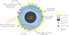Fig. 1

Schematic depicting all nondiffusive chemistry processes included in Pegasis.

2.4 Chemisorption

Thus far, all chemical processes considered have involved surface species that are physisorbed from the gas phase to the grain surface. As discussed earlier, molecules are bound to physisorption sites via weak electrostatic forces, making them susceptible to desorptive processes in high temperature environments (>100 K). To study the effects of surface chemistry at these temperatures, we include a new variant of surface species in our model, which behaves differently from species that undergo physisorption. This distinction arises from treating physisorption and chemisorption sites separately, based on the different binding energies with which molecules attach to the surface (Cazaux & Tielens 2002). As with nondiffusive chemistry, we consider various mechanisms through which chemisorption can occur, and the formulation is primarily based on the work of Acharyya et al. (2020), from which we also obtain the reaction set for each mechanism.

Similarly to diffusive reactions at physisorption sites, we allow surface reactions as well as reactive desorption processes through the chemisorbed sites in an almost identical manner. As with all chemisorption mechanisms, these rates are only calculated when the grain temperature exceeds 100 K. We implement all processes described for physisorbed species for each diffusive chemistry reaction involving chemisorbed species included in our network. In summary, all chemical processes (except nondiffusive chemistry) involving grain surfaces and grain mantles are depicted schematically in Figure 2.

3 Benchmarking PEGASIS

We benchmarked Pegasis against the public version of Nautilus used in RWH16. We ran both codes under the same physical conditions and settings, using the 2014 and 2024 releases of the KIDA network. Because many processes, such as nondiffusive chemistry and chemisorption, are unique to Pegasis, these were excluded from our comparison models. For this benchmark, we adopted typical cold core conditions for our physical parameters. The gas number density was taken as n_H = 3 × 10₄ cm⁻³. We assumed a temperature of 10 K for both gas and grains and a visual extinction of 15 mag. The standard cosmic-ray ionization rate ζ_H₂ of 1.3 × 10⁻¹⁷ s⁻¹ was assumed. Additionally, we allowed photodesorption and self-shielding for H₂, CO, and N₂. Quantum tunneling was not considered in this comparison; only thermal diffusion was allowed. We assumed spherical grains with a radius of 0.1 μm and density 3 g cm⁻³, with a dust-to-gas mass ratio of 0.01. Following RWH16, 10⁶ surface sites per grain were assumed and the ratio of diffusion barrier to binding energy was set to 0.4 for surface species and 0.8 for mantle species. Initial elemental abundances were adopted from RWH16. All models were run for 1 Myr.

We also used our model to investigate differences between the 2014 and 2024 releases of the KIDA chemical network for key species. The comparison is discussed in Appendix B. This benchmarking demonstrates that Pegasis and Nautilus show excellent agreement when using identical initial conditions and chemical networks to simulate cold core conditions.

Table 1

Processes included in each model presented in this work.

4 Model predictions using different approaches

To explore the different mechanisms used in the literature to simulate three-phase chemistry and to assess the effect of nondiffusive chemistry, we consider four different cold dense cloud models (Table 1). The goal is to identify the model that provides the best agreement with observed abundances in TMC-1. The physical conditions are adopted from Fuente et al. (2019), with gas number density n_H = 3 × 10⁴ cm⁻³, gas and grain temperatures = 10 K, visual extinction A_V = 15 mag, and ζH₂ = 1.3 × 10⁻¹⁷ s⁻¹. Following Wakelam et al. (2024), we use a larger value of 2.5 Å for the diffusion barrier thickness than was assumed in the benchmark models. As before, we assume spherical grains with a radius of 0.1 μm and a material density of 3 g cm⁻³, with a dust-to-gas mass ratio of 0.01. The surface site density is set to 1.5 × 10¹⁵ cm⁻². Following RWH16, the ratio of diffusion barrier to binding energy is set to 0.4 for the surface and 0.8 for the mantle. All species are allowed to diffuse both thermally and via quantum tunneling. Photodesorption and cosmic-ray sputtering are also enabled for all models. For chemical desorption, we use the prescription from Riedel et al. (2023), as it accounts for the nature of the desorbing surface. Finally, the initial elemental abundances are taken from Vidal et al. (2017), with all elements in atomic form except hydrogen, which is assumed to be entirely in molecular form from the start. All models are run for 10 Myr.

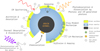Fig. 2

Schematic depicting all ice chemistry processes included in Pegasis, excluding nondiffusive chemistry.

Fig. 3

Evolution of ice thickness represented as the total number of layers across major ice species, for all the models. Contributions were calculated by accounting for the abundances of both surface and mantle species. The top row shows models with diffusive chemistry and the bottom row shows models with nondiffusive chemistry.

4.1 Comparing three-phase chemistry prescriptions

In this section, we explore the effect of the two three-phase chemistry prescriptions on the growth of ices, and how nondiffusive chemistry can further influence the contributions of different species. Figure 3 shows the total number of layers formed by major ices for each model included in this work. The total number of layers is calculated by dividing the ice concentrations (for both surface and mantle) by the total number of sites available per gas-phase molecule. We note that the original implementation of HH93 did not consider active mantle chemistry; however, in all our models, mantle species participate in all possible chemical reactions and photoprocesses.

Both three-phase prescriptions show a very similar distribution of major ices. H₂O and CO ices are the most dominant, making up bulk of the ice thickness. We observe that diffusive models with the three-phase prescriptions of RWH16 and HH93 produce a similar amount of ice layers, although the distribution across different ice species is notably different. There is much more CH₄ ice in M1 compared to M2, and the CO abundance does not decline after 1 Myr in case of M2, as it does for M1. Moreover, these trends remain similar when nondiffusive chemistry is activated in M3 and M4 (see Section 4.4 for discussion). As noted earlier, in the case of RWH16, molecules are immediately available for desorption as soon as the molecule above them leaves the surface, independent of the next event.

The individual contributions of major ices are sensitive to different chemical processes that can be included or excluded in a model run, as well as to the chemical network, as these factors affect chemistry by altering the dominant production pathways of these ices. For instance, RWH16, discussed the effects of reaction-diffusion competition on ice thickness variability.

To investigate the differences between the two prescriptions quantitatively, we examined the evolution of surface layers and mantle layers individually over the simulation time (Figure 4), for models with and without nondiffusive chemistry. We note that the number of mantle layers evolves similarly for both prescriptions, but the surface layers saturate at different values. This is expected, as HH93 does not account for surface thickness, whereas RWH16 includes it by considering the two outermost layers as part of the surface, following Fayolle et al. (2011). In HH93, the active surface layers are modeled through the core coverage factor α: $α_{gain} = \frac{\sum_{p} n_{s} (p)}{N_{site}},$ $\alpha_{\text{gain}} = \dfrac{\sum _{p}n_{\text{s}} (p)}{ N_{\text{site}}},$ (26)

where the numerator represents the total surface abundance and N_site is the total number of sites on a grain. Another key difference between the two prescriptions is that the movement of material between grain surface and grain mantle is based solely on the conservation of mass in the case of HH93, whereas RWH16 adopts the recommendation from Garrod (2013), in which the transfer rates are modeled through the thermal hopping (diffusion) timescales of the mantle molecules. Due to the absence of a buffer in which the outer monolayers are considered part of the surface in HH93, the heavier species are progressively trapped in the mantle. At late times, both accretion and desorption rates decrease, as there is not enough material from the gas phase to accrete onto the grain surfaces. The species locked in the mantle have longer desorption timescales as they must first transition to the surface. In addition, for HH93, mantle-to-surface transitions depend on desorption rates, rather than hopping rates, and these rates are much lower at late times compared to RWH16. This affects the heavier species much more than the three lightest species, H, H₂, and He, which have low binding energies that facilitate high desorption rates (Govers et al. 1980). In our models, we allow direct desorption from mantles through the process of cosmic-ray sputtering. This process brings mantle species back to the gas phase, without their having to first move to the surface layer. For both prescriptions, as adsorption and desorption decline on the surface over time, species continue to migrate from the surface to the mantle, leading to saturation of surface abundances after t > 10⁵ yr. In the case of RWH16, the surface roughness assumption acts as a buffer for grain surface chemistry to proceed and saturate after completely occupying the outer active monolayer region. Finally, we briefly note that the two prescriptions produce significant differences for models with and without nondiffusive chemistry (models M3 and M4 in Figure 3) which are discussed in more detail in Section 4.4.

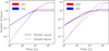Fig. 4

Evolution of ice thickness as a function of the number of surface and mantle layers individually, for models without nondiffusive chemistry (left) and with nondiffusive chemistry (right).

4.2 Gas compositions in TMC-1

In this section, we focus on reproducing the gas-phase chemical abundances observed in the well-studied TMC-1 (CP) (Kaifu et al. 2004; Gratier et al. 2016; Agúndez & Wakelam 2013). All observations were reported as column densities and then converted to abundances with respect to atomic hydrogen, assuming N(H₂) = 10²² cm⁻² (Cernicharo & Guelin 1987; Gratier et al. 2016).

The models in Table 1 share the same physical and chemical conditions but differ in their choice of three-phase chemistry prescription and the inclusion or exclusion of nondiffusive chemistry. The goal is to determine which of the four models best reproduces the observations, and to estimate the chemical age of the source (see, for instance, Majumdar et al. 2017). According to Smith et al. (2004) and Wakelam et al. (2024), abundances are considered well reproduced if they fall within one order of magnitude of the observed value. Several statistical methods have been employed by various authors to estimate how well a model reproduces observations. Wakelam et al. (2024) employ the distance-of-disagreement method, in which the best-fitting time corresponds to the minimum value of the parameter D. $D (t) = \frac{1}{N_{i}} \sum_{i} | \log (X_{mod, i} (t)) - \log (X_{obs, i}) |,$ $D(t) = \dfrac{1}{N_i} \sum_i \left | \log(X_{\text{mod},i}(t)) - \log(X_{\text{obs},i}) \right |,$ (27)

where X_mod,i (t) is the modeled abundance of species i at time t and X_obs,i is the observed abundance of species i from an observation dataset (Agúndez & Wakelam 2013 or Gratier et al. 2016). This method performs well in estimating the best-fitting time, but it is susceptible to large outliers and would be more robust if uncertainties for all observations were readily available. The mean logarithmic differences approach proposed by Loison et al. (2013) and Wakelam et al. (2015) suffers from a similar limitation.

Instead, we adopt the mean confidence level approach discussed in Garrod et al. (2007), which is well suited for our case and has also been applied in Majumdar et al. (2017) and RWH16. For this, we define confidence level κ_i as $κ_{i} = erfc (\frac{\log (X_{mod, i}) - \log (X_{obs, i})}{\sqrt{2} σ}),$ $\kappa_i = \text{erfc} \left( \dfrac{\log(X_{\text{mod},i}) - \log(X_{\text{obs},i})}{\sqrt{2}\sigma} \right),$ (28)

where erfc is the complementary error function, and we take σ = 1, implying that one standard deviation corresponds to the modeled value being within one order of the observed value, following Garrod et al. (2007). We calculate κ_i for each species at each time and the overall confidence at each time is defined as the mean of the individual levels for all species. We plot the mean confidence level for each model in Figure 5 for both observation datasets. For this analysis, we consider all models in Table 1 over a period of 10 Myr.

Our results are similar to those of Garrod et al. (2007) in that they produce two distinct local maxima for the mean confidence level, and therefore provide two options for the best-fitting time. The first local maximum for all models with respect to both observation sets is much flatter and represents a considerably larger interval, ranging from approximately 4 × 10⁴ yr to 2 × 10₅ yr. The models M1 and M3 produce higher mean confidence levels at late times (on the order of several 10⁶ yr), although Hartquist et al. (2001) suggest that TMC-1 is a relatively young molecular cloud with an estimated age of <10⁵ yr for TMC-1 Core D. However, according to Hartmann et al. (2001) and Mouschovias et al. (2006), an age of several 10⁵ yr is too short, as some estimates place the age of these dense clouds in the range of 10⁶-10⁷ yr. In more recent work, Navarro-Almaida et al. (2021) suggest that observations of TMC-1 (CP) can be best explained with a gravitational collapse model (t ~ 1 Myr) or a more sophisticated collapse model with ambipolar diffusion (t ~ 10 Myr). Nevertheless, we note that the late best-fitting times for models M1 and M3 are in agreement with the best times found by Wakelam et al. (2024). For the HH93 (M2 and M4) models, we were unable to find a definitive maximum at late times with either of the observational datasets of Agúndez & Wakelam (2013) or Gratier et al. (2016). For M1 and M3 (i.e., the RWH16 models), where we do observe a peak after 1 Myr, we note that the confidence level value for these late times exceed the value for early time.

Cases in which we note the confidence still increasing beyond 10 Myr suggest limitations of our model. These limitations can be attributed to both the chemical network and the individual chemical processes considered in our model. Moreover, our model is pseudo-time dependent, with physical conditions remaining constant throughout the evolution of the cloud. In reality, these environments are much more complex, with processes such as turbulence, shocks, and evolving densities due to core collapse affecting the chemical timescales. Therefore, in cases where the statistical methods fail to produce the best time within reasonable limits, authors such as Garrod et al. (2007) have opted to discard the models on physical and chemical grounds. The effects of nondiffusive chemistry on estimating chemical ages within the 10 Myr range is discussed in Sect. 4.4.

Overall, as is evident from Figure 6, the RWH16 model M1, can reproduce the observed abundances for the largest number of species: 23 out of32 gas-phase species from Gratier et al. (2016) and 47 out of 61 gas-phase species from Agúndez & Wakelam (2013), with best-fitting times of 4 and 3 Myr, respectively, within a factor of ten. Note that when creating Figure 6, observations with lower or upper limits were excluded. Upon including these observations, M1 reproduces 28 out of 37 gas-phase species abundances for Gratier et al. (2016) (confidence of 52%) and 48 out of 70 gas-phase species from Agúndez & Wakelam (2013) (confidence of 53%). The nondiffusive RWH16 model M3 also produces similar best-fitting times to M1, albeit with lower mean confidence. The HH93 models M2 and M4, despite producing higher confidence levels (as high as 56% for M4) at late times, failed to attain a maximum within 10 Myr.

This ambiguity in determining the best-fitting times is expected due to the complex structure of TMC-1, as well as the distinct physical history of its substructures. The time at which the mean confidence reaches a maximum is also sensitive to the assumed conditions, particularly the initial C/O ratio (Agúndez & Wakelam 2013). The role of desorption mechanisms in estimating chemical ages through modeling has been emphasized several times (Herbst 1995, 2001; Garrod et al. 2006). Finally, the choice of chemical networks can also influence the overall agreement with observations and yield different best-fitting times (Wakelam et al. 2024).

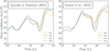Fig. 5

Mean confidence level (%) for the fit between different models and observations from the TMC-1 molecular cloud. Solid lines represent models without nondiffusive chemistry, while dashed lines correspond to models with nondiffusive chemistry.

4.3 Ice compositions

Ice compositions have been observed in absorption along the line of sight towards background stars, massive young stellar objects (MYSOs), and low-mass young stellar objects (LYSOs). Here, we compare observations of these objects with our model predictions. We use the ice abundances at the best-fit age for gas-phase observations of TMC-1. The observations and model abundances (relative to those of water ice) are given in Table 2. We include both surface and mantle abundances in the model predictions. In addition to the interstellar sources, we also include the abundances from cometary bodies in our comparison.

In this section, we discuss the results of model M1 and M2 for major ice species. Models M3 and M4, which involve nondiffusive chemistry, are discussed in the next section. Table 2 clearly shows that nondiffusive chemistry can significantly impact the contribution of different ice species to the total ice, the differences are evident between M1 and M3 and between M2 and M4. The sources and objects considered in this section are more evolved than TMC-1 and exhibit different physical conditions. They have also undergone significant processing and evolution as their physical conditions have changed; hence, we do not expect good agreement with the models. However, this comparison highlights how different the ice inventories are for molecular clouds compared to these sources. This can provide clues as to how different species are preserved, destroyed, or converted into other species as the cloud evolves and collapses to form protostellar objects.

In model M1, we observe that CO ice is nearly on par with H₂O, which is expected in certain scenarios in dense clouds. This is in agreement with RWH16, in which CO ice was produced at levels similar to H₂O ice when competition between diffusive reaction, desorption, and accretion was taken into account. In fact, in M2, the abundance of CO ice far exceeds that of H₂O. In our case, assuming a diffusion barrier thickness of 2.5 Å (Wakelam et al. 2024), the reaction pathway OH + CO → CO₂ + H is two orders of magnitude more efficient than O + HCO → CO₂ + H, consistent with Garrod & Pauly (2011).

However, this is still insufficient to drive the conversion of CO ice into CO₂, as accretion of CO is two orders of magnitude higher than that of CO₂ at this time. For all ice species in model M1, the dominant rates typically involve the movement of molecules between the ice surface and the mantle. The overprediction of CH₄ ice is also noteworthy. The H + CH₃ → CH₄ reaction emerges as the most important for the formation of CH₄ ice on the grain surface, consistent with the experimental results of Qasim et al. (2020). In contrast, model M2 does not exhibit this overprediction of ice. This difference can be attributed to inefficient movement of the ices from the mantle to the surface at late times in the HH93 model. The disparity in H₂CO and other ice abundances between models M1 and M2 in Table 2 can be explained in a similar way.

The differences in abundances detected in the sources in Table 2 suggest that, at the best-fitting time, this model had not attained the expected ratios for most ices with respect to H₂O ice. In addition, these ratios only provide part of the picture. The abundances relative to n_H, can also be derived from the corresponding column densities, as in Boogert et al. (2015). Our model predicts these abundances for TMC-1 within one order of magnitude of those observed, suggesting that over the course of evolution from clouds to protostellar objects, the changes occur mostly in the ratios in which these species exist as ices.

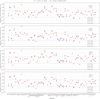Fig. 6

Ratios of modeled abundances to observed abundances for each model, for both datasets used in this work. Only species without upper or lower limits are shown. The number of species reproduced by each model is indicated for the datasets of Gratier et al. (2016) (blue) and Agúndez & Wakelam (2013) (red).

Table 2

Observed ice compositions in various massive young stellar objects (MYSOs), low-mass young stellar objects (LYSOs), and background (BG) stars, along with a Kuiper Belt comet, compared with model predictions at the best-fitting times derived from gas-phase abundances.

4.4 Effects of nondiffusive chemistry

Nondiffusive chemistry facilitates the formation of COMs. As evident in Figure 3, it does not necessarily increase the total ice content; rather, it helps in the formation of COMs from precursors such as methanol. The abundance of ices such as CH₄, CH₃OH, HCOOH, and HCOOCH₃ increases in both M3 and M4 models (Figure 3). In fact, the total number of ice layers decreases with the HH93 three-phase chemistry prescription and increases with the RWH16 prescription. In model M3, water ice rapidly accumulates shortly after 1 Myr of evolution, a trend that is absent in model M4. Specifically, nondiffusive photodissociation-induced reactions in M3 are more efficient than those in M4 at producing water ice in the grain mantle. The formation of water ice can be attributed to the following reactions: $b - H_{2} + b - O H \to b - H_{2} O + b - H$ $\ce{b-H2 + b-OH -> b-H2O + b-H}$ (R1) $b - C H_{4} + b - O H \to b - C H_{3} + b - H_{2} O$ $\ce{b-CH4 + b-OH -> b-CH3 + b-H2O}$ (R2)

The prefix ‘b-’ denotes a species located in the bulk (mantle). Reaction R1 proceeds through a diffusive pathway, as b-H₂ is light enough to diffuse readily in cold environments (approximately ~10 K). In contrast, Reaction R2 primarily proceeds via nondiffusive pathways. Both of these reactions exhibit significantly lower rates in model M4. The insufficient abundance of methane ice in the HH93 models largely explains the inefficiency of Reaction R2. Furthermore, the inclusion of nondiffusive chemistry increases the abundance of CO₂ ice in both models M3 and M4, as its production no longer relies on the very slow diffusion of CO and O at the low temperature of 10 K. Nondiffusive chemistry enables the formation of CO₂ without requiring diffusion, in agreement with the findings of Jiménez-Serra et al. (2025), in which models with nondiffusive chemistry produced CO₂ ice even at low temperatures of T_dust < 12 K.

Figure 4 shows that nondiffusive chemistry does not affect the distribution between surface and mantle abundances under a three-phase prescription. Enabling nondiffusive chemistry not only significantly alters the abundances of major ice species across all models (see Table 2), but also enhances the abundances of COMs in each case. In the case of HH93, nondiffusive chemistry may result in a best-fitting time closer to previous estimates of several Myr. This may be attributed to the additional formation pathways provided by nondiffusive chemistry, which produce heavier COMs that are susceptible to getting trapped in the mantle. These pathways can compensate for the lower surface abundances characteristic of HH93. Given that the effects and trends of nondiffusive chemistry are consistent across all models, we focus our discussion and results on the RWH16 models for brevity.

4.4.1 On COMs in the gas-phase

Figure 7 shows the abundances of various oxygen-bearing COMs in the gas-phase that have been detected in TMC-1 and are included in the 2024 KIDA network, as well as methylamine (CH₃NH₂). This evolution of abundances can be divided into three epochs: the early stage (from the beginning to 10² yr), the middle stage (10² yr to 10⁴ yr), and the late stage (beyond 10⁴ yr). Owing to these three distinct evolutionary stages, we observe significant effects on the abundances of methanol (CH₃OH), ethanol (CH₃CH₂OH), dimethyl ether (CH₃OCH₃), and methyl formate (HCOOCH₃) during the early stage, while the abundances of the remaining species show only marginal differences between the models with and without nondiffusive chemistry. In the middle stage, ethanol exhibits the greatest deviation from the diffusive-only chemistry when nondiffusive mechanisms are included. In the late stage, which encompasses the best-fitting time, the differences for all species gradually decrease as their abundances converge toward steady state. We note that for species such as propenal (C₂H₃CHO), acetone (CH₃COCH₃), and propanal (C₂H₅CHO), the negligible differences across all stages can be attributed to their limited chemical reactions in the 2024 KIDA network. Specifically, propenal has no grainsurface reaction (diffusive or nondiffusive), acetone has only one pathway, and propanal has just two.

In our model, most gas-phase COMs are primarily produced on the grain surface and subsequently desorbed into the phase via chemical desorption, following the prescription of Riedel et al. (2023). Among pathways involving only gas-phase species, dissociative recombination emerges as the sole reaction mechanism. The destruction of gas-phase COMs is primarily driven by a single mechanism of proton-transfer, where ions such as H₃⁺ and H₃O⁺ act as primary proton donors.

Diffusive chemistry dominates over nondiffusive mechanisms for gas-phase COMs, whose major formation pathway involves successive hydrogenation on the grain surface followed by reactive desorption, as the lone H atom is light enough to diffuse efficiently at low temperatures of ~10 K. For example, CH₃OH is most efficiently produced via diffusive hydrogenation of both the methoxy (CH₃O) and hydroxymethyl (CH₂OH) radicals, each contributing approximately 44% to the overall formation. However, in the case of heavier COMs such as ethanol (CH₃CH₂OH), whose major pathway (~55%) is $s - C H_{3} + s - C H_{2} O H \to s - C H_{3} C H_{2} O H \to C H_{3} C H_{2} O H$ $\ce{s-CH3 + s-CH2OH -> s-CH3CH2OH -> CH3CH2OH} \tag{R3}$ (R3)

where both reactants are heavy molecules, the nondiffusive pathway dominates. The prefix ‘s-’ denotes a ice species on the grain surface. This trend is observed for all COMs shown in Figure 7. However, the relative contribution of each chemical process -gas-phase, grain-surface diffusive, or grain-surface nondiffusive - is time-dependent. For instance, acetaldehyde (CH₃CHO) forms primarily (~53%) via a nondiffusive grain-surface reaction between s-CH₃ and s-HCO at the best-fitting time of 4 Myr. The formation of acetone (CH₃COCH₃), methyl formate (HCOOCH₃), and methylamine (CH₃NH₂) is notably dominated by gas-phase processes. Specifically, these molecules are primarily produced via dissociative recombination of their respective protonated precursors - C₃H₆OH⁺ for acetone (~54%), H₅C₂O₂⁺ for methyl formate (~80%), and CH₃NH₃⁺ for methylamine (~69%) at the best-fitting time of 4 Myr. Finally, propanal (C₂H₅CHO) is forms first on the grain surface through a nondiffusive reaction and subsequently desorbs into the gas phase via chemical desorption. Rather than forming through hydrogenation, propanal forms via the addition of atomic oxygen to propene (CH₃CHCH₂).

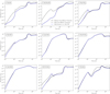Fig. 7

Gas-phase abundances of major COMs as a function of time for models with (M3) and without (M1) nondiffusive chemistry.

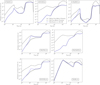Fig. 8

Abundances of major COM ices as a function of time with (M3) and without (M1) nondiffusive chemistry.

4.4.2 On COMs in the ice-phase

We concentrate our discussion on a subset of the COMs listed in Table 2 as they have been detected in MYSOs, LYSOs, and cometary bodies, as well as on some oxygen-bearing COMs detected in prestellar cores such as L1689B, L1544, and B1-b (Bacmann et al. 2012; Cernicharo et al. 2012; Vastel et al. 2014). The evolution of their fractional abundances relative to water ice is shown in Figure 8.

To form methanol (s-CH₃OH) on the grain surface, without nondiffusive chemistry, two main pathways exist: $s - H + s - C H_{3} O \to s - C H_{3} O H$ $\ce{s-H + s-CH3O -> s-CH3OH}$ (R4) $s - H + s - C H_{2} O H \to s - C H_{3} O H$ $\ce{s-H + s-CH2OH -> s-CH3OH}$ (R5)

Reaction R4 represents the final step in the successive hydrogenation of s-CO to form methanol, whereas reaction R5 corresponds to hydrogenation of the hydroxymethyl radical, which itself originates from H-abstraction of methanol. With nondiffusive chemistry, the reaction s-OH + s-CH₃ → s-CH₃OH also becomes significant via the three-body nondiffusive reaction, although its contribution remains below 1%. This is similar to the findings of Jiménez-Serra et al. (2025), who found that this pathway produces methanol only marginally, even in models incorporating nondiffusive chemistry. Overall, the Eley-Rideal nondiffusive reactions dominate all other pathways forming methanol. The destruction of s-CH₃OH is also strongly influenced by the inclusion of nondiffusive chemistry. In the diffusive-only scenario, methanol is destroyed by reacting with atomic hydrogen, leading to the formation of the hydroxy-methyl group (s-CH₂OH) or methoxide (s-CH₃O). Both processes are enhanced by three-body and Eley-Rideal nondiffusive mechanisms. Notably, nondiffusive chemistry destroys methanol on grain surfaces more efficiently than photoprocesses.

For formic acid (s-HCOOH), nondiffusive chemistry greatly enhances the main pathway s-H + s-HOCO → s-HCOOH, with s-OH + s-HcO → s-HCOOH also contributing sub stantially. The latter reaction proceeds through all nondiffusive mechanisms (Eley-Rideal, three-body and photodissociation-induced nondiffusive mechanisms) included in our model and is much more efficient than the diffusive counterpart. Turning on nondiffusive chemistry also enhances the rates of diffusive reactions, as more ices become available to react on grain surfaces. For acetaldehyde (s-CH₃CHO), the main formation pathways $s - C H_{3} + s - H C O \to s - C H_{3} C H O$ $\ce{s-CH3 + s-HCO -> s-CH3CHO}$ (R6) $s - H + s - C H_{3} C O \to s - C H_{3} C H O$ $\ce{s-H + s-CH3CO -> s-CH3CHO}$ (R7)

We note that R6 is more efficient through the nondiffusive channel and R7 dominates for diffusive chemistry. The inclusion of nondiffusive chemistry also enhances acetaldehyde destruction pathways, supplementing conventional photoprocesses and diffusive reactions. All nondiffusive mechanisms are more efficient than photoprocesses but less so than diffusive pathways.

The case of dimethyl ether (CH₃OCH₃) is more interesting, as it is produced through the following three-body excited nondiffusive reaction (represented as two successive two-body reactions): $s - C H^{⋆} 3 + s - H_{2} C O \to s - C H_{3} O C H_{2}$ $\ce{s-CH^{\star}3 + s-H2CO -> s-CH3OCH2}$ (R8) $s - H + s - C H_{3} O C H_{2} \to s - C H_{3} O C H_{3} .$ $\ce{s-H + s-CH3OCH2 -> s-CH3OCH3}.$ (R9)

Reaction R9 proceeds via this mechanism at a much higher rate than its diffusive counterpart due to the involvement of excited s-CH^★₃ ice in R8. The reaction s-CH₃ + s-CH₃O → s-CH₃OCH₃ represents other major pathway for forming dimethyl ether on grain surfaces. Production of ethanol (s-CH₃CH₂OH) is almost negligible without nondiffusive chemistry, but increases significantly via the reaction of more readily available hydroxy-methyl (s-CH₂OH) with s-CH₃ ice. Notably, enabling nondiffusive chemistry suppresses the corresponding diffusive reaction. Similarly, production of s-HCOOCH₃ via reaction of methoxide (s-CH₃O) with s-HCO becomes much more feasible with nondiffusive chemistry, while the diffusive pathway is suppressed. Although nondiffusive chemistry produces the smallest abundance differences for methylamine (s-CH₃NH₂), a new pathway in the form of s-NH₂ + s-CH₃→s-CH₃NH₂ emerges as a major route to form this nitrogenbearing COM.

We performed the same analysis using model M1 with ER chemistry from Ruaud et al. (2015) and found it less efficient than nondiffusive chemistry in producing the COMs discussed here (Figure 8).

5 Conclusions

In this work, we present a new and flexible astrochemical code that offers numerous choices and options for exploring the effects of different chemical processes under varying physical conditions in the interstellar medium. The key findings are summarized below.

Our benchmarking with well-established models, such as Nautilus, reveals excellent agreement, while also highlighting the key differences between the latest 2024 KIDA network and the previously released 2014 version. It also establishes the importance of reproducing identical results from identical initial conditions, demonstrating the robustness and stability of the numerical methods used in Pegasis.
The importance of grain surface chemistry in cold cores suggests that the three-phase prescription of RWH16 captures surface processes slightly better than that of HH93, due to higher concentrations of species on the surface.
We find that current networks still lack the ability to unambiguously reproduce the gas-phase observations of TMC-1 (CP). This can be attributed to multiple factors discussed in Wakelam et al. (2024) regarding uncertainties in the chemical network. We select the late time as the best-fitting epoch because it provides the higher mean confidence.
The significance of desorption cannot be understated when estimating chemical ages. Previous works, such as Garrod et al. (2006), have emphasized its importance; the process is sensitive to the reaction network and the types of desorptive processes considered.
Comparison with ice abundances observed toward BG stars, MYSOs, LYSOs, and cometary bodies provides insight into the chemical inventory’s transformation as cloud collapses toward more evolved protostellar stages.
We explore the effects of all nondiffusive mechanisms included in our model on the abundances of COMs, noting that major reactions are greatly enhanced when nondiffusive chemistry is enabled, thereby increasing the share of COMs in both surface and bulk ice.
For gas-phase COMs, nondiffusive mechanisms emerge as the dominant pathways for their formation on grain surfaces, followed by chemical desorption - especially when the involved reactants are heavier than atomic hydrogen -and thus do not diffuse efficiently at the low temperatures typical of cold cores.
Nondiffusive chemistry also affects the diffusive chemistry, sometimes negatively and positively, depending on the molecule. The Eley-Rideal and three-body nondiffusive mechanisms are consistently more efficient than photodissociation-induced nondiffusive reactions, all of which have higher rates than their diffusive counterparts across COMs.
The more general treatment of Eley-Rideal chemistry via nondiffusive means, as opposed to the carbon-specific treatment of the Eley-Rideal process in Ruaud et al. (2015), leads to a better estimation of COM abundances in cold cores.
The inclusion of nondiffusive chemistry alongside chemisorption makes Pegasis an extremely versatile astrochemical code, enabling simulations of diverse astrochemical environments with varying grain-surface chemistry and processes. These environments may correspond to cold cores (as studied here) or high-temperature regions (>100 K), which we will explore in a future study.

Acknowledgements

L.M. expresses his sincere thanks to Valentine Wakelam for permitting the use of the Nautilus gas-grain three-phase chemical code in the past, for allowing a detailed benchmark comparison with Pegasis in this work, and for encouraging the independent development of this new, fast, Python-based astrochemical code within his group. L.M. also thanks Ewine F. van Dishoeck for valuable discussions in the past related to the role of nondiffusive chemistry. L.M. acknowledges financial support from DAE and the DST-SERB research grant (MTR/2021/000864) from the Government of India for this work. This research was carried out in part at the Jet Propulsion Laboratory, which is operated for NASA by the California Institute of Technology. K.W. acknowledges the financial support from the NASA Emerging Worlds grant 18-EW-182-0083. We would like to thank the anonymous referee for constructive comments that helped improve the manuscript.

Appendix A Generation of nondiffusive reactions

To generate the reaction set for each nondiffusive mechanism discussed in the work, we start with grain-surface and bulk-ice reactions of the 2024 KIDA network. To generate the set for photodissociation-induced nondiffusive reactions, we identify all the species which are produced through photodissociations by UV photons on grain surfaces and photodissociations by cosmic-ray induced UV photons on grain surfaces. These are the type 17, 18, 19, 20 in the reaction network (Wakelam et al. 2024). Once we have these photoproducts, we move to type 14 which represents all diffusive reactions, to identify the subset of reactions where the photoproducts participate as reactants, giving us the required reaction set. In the case of nondiffusive Eley-Rideal reactions, similar process is performed, except this time, we take products from type 99, which represents adsorption reactions on grains. In the subset of diffusive reactions where these products occur as reactants, it ensures that one reactant has already accreted on the grain-surface and it immediately encounters the other reactant there. Further, we ensure that the complete reaction is a surface-only process with no bulk-ice species involved, as is the case with E-R. Finally, to generate the nondiffusive three-body reactions, we need to select the subset of diffusive reactions for both grain-surface and grain-mantle where both involved reactants occur as products of diffusive reactions itself. To this end, we take products from type 14, and then proceed similar to previous cases to generate the reaction set for this mechansim. The following two grain-surface reactions are added separately for the three-body excited formation mechanism (Jin & Garrod 2020) $s - C H^{⋆} 3 + s - C O \to s - C H_{3} C O$ $\ce{s-CH^{\star}3 + s-CO -> s-CH3CO}$ (AR1) $s - H + s - C H_{3} C O \to s - C H_{3} C H O$ $\ce{s-H + s-CH3CO -> s-CH3CHO}$ (AR2)

and $s - C H^{⋆} 3 + s - H_{2} C O \to s - C H_{3} O C H_{2}$ $\ce{s-CH^{\star}3 + s-H2CO -> s-CH3OCH2}$ (AR3) $s - H + s - C H_{3} O C H_{2} \to s - C H_{3} O C H_{3}$ $\ce{s-H + s-CH3OCH2 -> s-CH3OCH3}$ (AR4)

under the constraint that s-CH₃^★ ice is formed by the following reaction $s - H + s - C H_{2} \to s - C H^{⋆} 3$ $\ce{s-H + s-CH2 -> s-CH^{\star}3}$ (AR5)

Jin & Garrod (2020) discuss an additional reaction that undergoes a nondiffusive process via the formation of an excited intermediate. However, this reaction was not included because one of its participants (s-CH₃OCO) is not present in the 2024 KIDA network.

Appendix B Benchmarking Pegasis

We depict time evolution of select species detected in TMC-1 (CP) using the both 2014 and 2024 KIDA networks with Pegasis and Nautilus. The oxygen-bearing species are shown in Figure B.1, with hydrocarbons in Figure B.2, nitrogen-bearing in Figures B.3, B.4 and sulfur-bearing species follow in Figure B.5. For visual clarity, the Nautilus results were over-plotted over Pegasis results through orange-colored markers. As is evident from the figures, Pegasis and Nautilus have excellent agreement, with the plots of both models exhibiting high co-incidence.

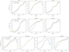Fig. B.1

Comparison of selected oxygen-bearing species in gas-phase detected in TMC-1 molecular cloud. Both PEGASIS (blue lines) and NAUTILUS (orange markers) have excellent agreement for both the networks (2014 is represented by dash-dotted lines and 2024 represented by solid lines).

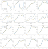Fig. B.2

Same as Figure B.1, but for hydrocarbons.

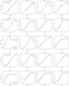Fig. B.3

Same as Figure B.1, but for nitrogen-bearing species.

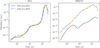Fig. B.4

Same as Figure B.1, but for NO-bearing species.

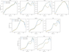Fig. B.5

Same as Figure B.1, but for sulfur-bearing species.

References

Acharyya, K., Schulte, S. W., & Herbst, E. 2020, ApJS, 247, 4 [Google Scholar]
Agúndez, M., & Wakelam, V. 2013, Chem. Rev., 113, 8710 [Google Scholar]
Agúndez, M., Marcelino, N., Tercero, B., et al. 2021, A&A, 649, L4 [NASA ADS] [CrossRef] [EDP Sciences] [Google Scholar]
Agúndez, M., Loison, J.-C., Hickson, K., et al. 2023, A&A, 673, A34 [NASA ADS] [CrossRef] [EDP Sciences] [Google Scholar]
Agúndez, M., Bermúdez, C., Cabezas, C., et al. 2024, A&A, 688, L31 [NASA ADS] [CrossRef] [EDP Sciences] [Google Scholar]
Agúndez, M., Molpeceres, G., Cabezas, C., et al. 2025, A&A, 693, L20 [NASA ADS] [CrossRef] [EDP Sciences] [Google Scholar]
Andersson, S., & van Dishoeck, E. 2008, A&A, 491, 907 [NASA ADS] [CrossRef] [EDP Sciences] [Google Scholar]
Bacmann, A., Taquet, V., Faure, A., Kahane, C., & Ceccarelli, C. 2012, A&A, 541, L12 [NASA ADS] [CrossRef] [EDP Sciences] [Google Scholar]
Balucani, N., Ceccarelli, C., & Taquet, V. 2015, MNRAS, 449, L16 [Google Scholar]
Bates, D. R., & Spitzer, Jr., L. 1951, ApJ, 113, 441 [NASA ADS] [CrossRef] [Google Scholar]
Bergner, J. B., Öberg, K. I., Garrod, R. T., & Graninger, D. M. 2017a, ApJ, 841, 120 [Google Scholar]
Bergner, J. B., Öberg, K. I., & Rajappan, M. 2017b, ApJ, 845, 29 [Google Scholar]
Boogert, A. C. A., Gerakines, P. A., & Whittet, D. C. B. 2015, ARA&A, 53, 541 [Google Scholar]
Cabezas, C., Agúndez, M., Marcelino, N., et al. 2025, A&A, 693, L14 [NASA ADS] [CrossRef] [EDP Sciences] [Google Scholar]
Cazaux, S., & Tielens, A. 2002, ApJ, 575, L29 [NASA ADS] [CrossRef] [Google Scholar]
Cernicharo, J., & Guelin, M. 1987, A&A, 176, 299 [NASA ADS] [Google Scholar]
Cernicharo, J., Marcelino, N., Roueff, E., et al. 2012, ApJ, 759, L43 [NASA ADS] [CrossRef] [Google Scholar]
Cernicharo, J., Cabezas, C., Agúndez, M., et al. 2024a, A&A, 688, L13 [NASA ADS] [CrossRef] [EDP Sciences] [Google Scholar]
Cernicharo, J., Cabezas, C., Fuentetaja, R., et al. 2024b, A&A, 690, L13 [NASA ADS] [CrossRef] [EDP Sciences] [Google Scholar]
Chang, Q., & Herbst, E. 2016, ApJ, 819, 145 [Google Scholar]
Collings, M. P., Anderson, M. A., Chen, R., et al. 2004, MNRAS, 354, 1133 [NASA ADS] [CrossRef] [Google Scholar]
Cuppen, H., Karssemeijer, L., & Lamberts, T. 2013, Chem. Rev., 113, 8840 [NASA ADS] [CrossRef] [Google Scholar]
Das, A., Majumdar, L., Sahu, D., et al. 2015, ApJ, 808, 21 [NASA ADS] [CrossRef] [Google Scholar]
Draine, B. T., & Sutin, B. 1987, ApJ, 320, 803 [NASA ADS] [CrossRef] [Google Scholar]
Du, F. 2021, Res. Astron. Astrophys., 21, 077 [NASA ADS] [CrossRef] [Google Scholar]
Fayolle, E. C., Öberg, K., Cuppen, H. M., Visser, R., & Linnartz, H. 2011, A&A, 529, A74 [NASA ADS] [CrossRef] [EDP Sciences] [Google Scholar]
Fuente, A., Navarro, D., Caselli, P., et al. 2019, A&A, 624, A105 [NASA ADS] [CrossRef] [EDP Sciences] [Google Scholar]
Fuentetaja, R., Agúndez, M., Cabezas, C., et al. 2024, A&A, 688, L15 [NASA ADS] [CrossRef] [EDP Sciences] [Google Scholar]
Furuya, K., Aikawa, Y., Hincelin, U., et al. 2015, A&A, 584, A124 [NASA ADS] [CrossRef] [EDP Sciences] [Google Scholar]
Furuya, K., Drozdovskaya, M., Visser, R., et al. 2017, A&A, 599, A40 [NASA ADS] [CrossRef] [EDP Sciences] [Google Scholar]
Garrod, R. 2008, A&A, 491, 239 [NASA ADS] [CrossRef] [EDP Sciences] [Google Scholar]
Garrod, R. T. 2013, ApJ, 765, 60 [Google Scholar]
Garrod, R. T., & Herbst, E. 2006, A&A, 457, 927 [NASA ADS] [CrossRef] [EDP Sciences] [Google Scholar]
Garrod, R. T., & Pauly, T. 2011, ApJ, 735, 15 [Google Scholar]
Garrod, R., Park, I. H., Caselli, P., & Herbst, E. 2006, Faraday Discuss., 133, 51 [Google Scholar]
Garrod, R. T., Wakelam, V., & Herbst, E. 2007, A&A, 467, 1103 [NASA ADS] [CrossRef] [EDP Sciences] [Google Scholar]
Geppert, W. D., & Larsson, M. 2008, Mol. Phys., 106, 2199 [Google Scholar]
Gould, R. J., & Salpeter, E. E. 1963, ApJ, 138, 393 [NASA ADS] [CrossRef] [Google Scholar]
Govers, T. R., Mattera, L., & Scoles, G. 1980, J. Chem. Phys., 72, 5446 [Google Scholar]
Gratier, P., Majumdar, L., Ohishi, M., et al. 2016, ApJS, 225, 25 [Google Scholar]
Gredel, R. 1990, in Molecular Astrophysics, ed. T. W. Hartquist (Cambridge: Cambridge University Press), 305 [Google Scholar]
Gredel, R., Lepp, S., & Dalgarno, A. 1987, ApJ, 323, L137 [Google Scholar]
Gredel, R., Lepp, S., Dalgarno, A., & Herbst, E. 1989, ApJ, 347, 289 [Google Scholar]
Hartmann, L., Ballesteros-Paredes, J., & Bergin, E. A. 2001, ApJ, 562, 852 [NASA ADS] [CrossRef] [Google Scholar]
Hartquist, T., Williams, D., & Viti, S. 2001, A&A, 369, 605 [NASA ADS] [CrossRef] [EDP Sciences] [Google Scholar]
Hasegawa, T. I., & Herbst, E. 1993a, MNRAS, 261, 83 [NASA ADS] [CrossRef] [Google Scholar]
Hasegawa, T. I., & Herbst, E. 1993b, MNRAS, 263, 589 [Google Scholar]
Hasegawa, T. I., Herbst, E., & Leukng, C. M. 1992, ApJS, 82, 167 [NASA ADS] [CrossRef] [Google Scholar]
Herbst, E. 1995, Annu. Rev. Phys. Chem., 46, 27 [Google Scholar]
Herbst, E. 2001, Chem. Soc. Rev., 30, 168 [CrossRef] [Google Scholar]
Herbst, E., & Klemperer, W. 1973, ApJ, 185, 505 [Google Scholar]
Herbst, E., & van Dishoeck, E. F. 2009, ARA&A, 47, 427 [NASA ADS] [CrossRef] [Google Scholar]
Herbst, E., Chang, Q., & Cuppen, H. M. 2005, J. Phys. Conf. Ser., 6, 18 [Google Scholar]
Hindmarsh, A. C. 1983, in IMACS Transactions on Scientific Computation, Scientific Computing, eds. R. S. S. et al. (Amsterdam: North-Holland), 1, 55 [Google Scholar]
Holbrook, K. A., Pilling, M. J., & Robertson, S. H. 1996, Unimolecular Reactions, 2nd edn. (Hoboken: Wiley) [Google Scholar]
Holdship, J., Viti, S., Jiménez-Serra, I., Makrymallis, A., & Priestley, F. 2017, AJ, 154, 38 [NASA ADS] [CrossRef] [Google Scholar]
Jiménez-Serra, I., Megías, A., Salaris, J., et al. 2025, A&A, 695, A247 [NASA ADS] [CrossRef] [EDP Sciences] [Google Scholar]
Jin, M., & Garrod, R. T. 2020, ApJS, 249, 26 [Google Scholar]
Kaifu, N., Ohishi, M., Kawaguchi, K., et al. 2004, Publ. Astron. Soc. Jpn., 56, 69 [Google Scholar]
Kalvāns, J. 2014, A&A, 573, A38 [Google Scholar]
Kalvāns, J., & Shmeld, I. 2010, A&A, 521, A37 [NASA ADS] [CrossRef] [EDP Sciences] [Google Scholar]
Katz, N., Furman, I., Biham, O., Pirronello, V., & Vidali, G. 1999, ApJ, 522, 305 [NASA ADS] [CrossRef] [Google Scholar]
Kooij, D. M. 1893, ZPhCh, 12U, 155 [Google Scholar]
Lam, S. K., stuartarchibald, Pitrou, A., et al. 2024, https://doi.org/10.5281/zenodo.11642058 [Google Scholar]
Le Teuff, Y. H., Millar, T. J., & Markwick, A. J. 2000, A&AS, 146, 157 [NASA ADS] [CrossRef] [EDP Sciences] [Google Scholar]
Lee, H. H., Herbst, E., Pineau des Forets, G., Roueff, E., & Le Bourlot, J. 1996, A&A, 311, 690 [Google Scholar]
Li, X., Heays, A. N., Visser, R., et al. 2013, A&A, 555, A14 [NASA ADS] [CrossRef] [EDP Sciences] [Google Scholar]
Loison, J.-C., Wakelam, V., Hickson, K. M., Bergeat, A., & Mereau, R. 2013, MNRAS, 437, 930 [Google Scholar]
Majumdar, L., Gratier, P., Ruaud, M., et al. 2017, MNRAS, 466, 4470 [Google Scholar]
Maret, S., Bergin, E., & Tafalla, M. 2013, A&A, 559, A53 [NASA ADS] [CrossRef] [EDP Sciences] [Google Scholar]
McElroy, D., Walsh, C., Markwick, A., et al. 2013, A&A, 550, A36 [NASA ADS] [CrossRef] [EDP Sciences] [Google Scholar]
McGuire, B. A. 2022, ApJS, 259, 30 [NASA ADS] [CrossRef] [Google Scholar]
Millar, T. J., Bennett, A., Rawlings, J. M. C., Brown, P. D., & Charnley, S. B. 1991, A&AS, 87, 585 [NASA ADS] [Google Scholar]
Millar, T. J., Farquhar, P. R. A., & Willacy, K. 1997, A&AS, 121, 139 [NASA ADS] [CrossRef] [EDP Sciences] [Google Scholar]
Millar, T., Walsh, C., Van de Sande, M., & Markwick, A. 2024, A&A, 682, A109 [NASA ADS] [CrossRef] [EDP Sciences] [Google Scholar]
Minissale, M., Dulieu, F., Cazaux, S., & Hocuk, S. 2016, A&A, 585, A24 [NASA ADS] [CrossRef] [EDP Sciences] [Google Scholar]
Mouschovias, T. C., Tassis, K., & Kunz, M. W. 2006, ApJ, 646, 1043 [Google Scholar]
Mumma, M. J., & Charnley, S. B. 2011, ARA&A, 49, 471 [NASA ADS] [CrossRef] [Google Scholar]
Navarro-Almaida, D., Fuente, A., Majumdar, L., et al. 2021, A&A, 653, A15 [NASA ADS] [CrossRef] [EDP Sciences] [Google Scholar]
Öberg, K. I., Fuchs, G. W., Awad, Z., et al. 2007, ApJ, 662, L23 [Google Scholar]
Öberg, K. I., Garrod, R. T., van Dishoeck, E. F., & Linnartz, H. 2009, A&A, 504, 891 [NASA ADS] [CrossRef] [EDP Sciences] [Google Scholar]
Prasad, S. S., & Tarafdar, S. P. 1983, ApJ, 267, 603 [Google Scholar]
Qasim, D., Fedoseev, G., Chuang, K. J., et al. 2020, Nat. Astron, 4, 781 [Google Scholar]
Rachid, M., van Scheltinga, J. T., Koletzki, D., & Linnartz, H. 2020, A&A, 639, A4 [NASA ADS] [CrossRef] [EDP Sciences] [Google Scholar]
Reboussin, L., Wakelam, V., Guilloteau, S., & Hersant, F. 2014, MNRAS, 440, 3557 [NASA ADS] [CrossRef] [Google Scholar]
Remijan, A. J., Changala, P. B., Xue, C., et al. 2025, ApJ, 982, 191 [Google Scholar]
Riedel, W., Sipilä, O., Redaelli, E., et al. 2023, A&A, 680, A87 [NASA ADS] [CrossRef] [EDP Sciences] [Google Scholar]
Roberge, W. G., Jones, D., Lepp, S., & Dalgarno, A. 1991, ApJS, 77, 287 [Google Scholar]
Rocha, W., van Dishoeck, E., Ressler, M., et al. 2024, A&A, 683, A124 [NASA ADS] [CrossRef] [EDP Sciences] [Google Scholar]
Ruaud, M., Loison, J., Hickson, K., et al. 2015, MNRAS, 447, 4004 [Google Scholar]
Ruaud, M., Wakelam, V., & Hersant, F. 2016, MNRAS, 459, 3756 [Google Scholar]
Rubin, M., Altwegg, K., Balsiger, H., et al. 2019, MNRAS, 489, 594 [Google Scholar]
Semenov, D., Hersant, F., Wakelam, V., et al. 2010, A&A, 522, A42 [NASA ADS] [CrossRef] [EDP Sciences] [Google Scholar]
Shen, C., Greenberg, J., Schutte, W., & Van Dishoeck, E. 2004, A&A, 415, 203 [NASA ADS] [CrossRef] [EDP Sciences] [Google Scholar]
Shingledecker, C. N., Tennis, J., Le Gal, R., & Herbst, E. 2018, ApJ, 861, 20 [Google Scholar]
Sipilä, O., Caselli, P., Redaelli, E., & Spezzano, S. 2022, A&A, 668, A131 [NASA ADS] [CrossRef] [EDP Sciences] [Google Scholar]
Smith, I. W., Herbst, E., & Chang, Q. 2004, MNRAS, 350, 323 [Google Scholar]
Sternberg, A., Dalgarno, A., & Lepp, S. 1987, ApJ, 320, 676 [NASA ADS] [CrossRef] [Google Scholar]
Taquet, V., Ceccarelli, C., & Kahane, C. 2012, A&A, 538, A42 [NASA ADS] [CrossRef] [EDP Sciences] [Google Scholar]
Terwisscha van Scheltinga, J., Ligterink, N., Boogert, A., Van Dishoeck, E., & Linnartz, H. 2018, A&A, 611, A35 [NASA ADS] [CrossRef] [EDP Sciences] [Google Scholar]
Terwisscha van Scheltinga, J. T., Marcandalli, G., McClure, M. K., Hogerheijde, M. R., & Linnartz, H. 2021, A&A, 651, A95 [NASA ADS] [CrossRef] [EDP Sciences] [Google Scholar]
Tielens, A. G. G. M., & Allamandola, L. J. 1986, Composition, Structure, and Chemistry of Interstellar Dust (Berlin: Springer) [Google Scholar]
Tielens, A. G. G. M., & Hagen, W. 1982, A&A, 114, 245 [Google Scholar]
Umebayashi, T. 1983, Prog. Theor. Phys., 69, 480 [Google Scholar]
Vastel, C., Ceccarelli, C., Lefloch, B., & Bachiller, R. 2014, ApJ, 795, L2 [NASA ADS] [CrossRef] [Google Scholar]
Vasyunin, A. I., & Herbst, E. 2013, ApJ, 769, 34 [Google Scholar]
Vasyunin, A. I., Caselli, P., Dulieu, F., & Jiménez-Serra, I. 2017, ApJ, 842, 33 [Google Scholar]
Vidal, T. H., Loison, J.-C., Jaziri, A. Y., et al. 2017, MNRAS, 469, 435 [NASA ADS] [CrossRef] [Google Scholar]
Vidali, G., Roser, J. E., Ling, L., et al. 2006, Faraday Discuss., 133, 125 [Google Scholar]
Visser, R., Van Dishoeck, E., & Black, J. H. 2009, A&A, 503, 323 [NASA ADS] [CrossRef] [EDP Sciences] [Google Scholar]
Wakelam, V., Herbst, E., Loison, J.-C., et al. 2012, ApJS, 199, 21 [Google Scholar]
Wakelam, V., Loison, J.-C., Herbst, E., et al. 2015, ApJS, 217, 20 [Google Scholar]
Wakelam, V., Dartois, E., Chabot, M., et al. 2021, A&A, 652, A63 [NASA ADS] [CrossRef] [EDP Sciences] [Google Scholar]
Wakelam, V., Gratier, P., Loison, J.-C., et al. 2024, A&A, 689, A63 [NASA ADS] [CrossRef] [EDP Sciences] [Google Scholar]
Watson, W. D. 1973, ApJ, 183, L17 [NASA ADS] [CrossRef] [Google Scholar]
Watson, W. D. 1974, ApJ, 188, 35 [NASA ADS] [CrossRef] [Google Scholar]
Watson, W. D. 1976, Rev. Mod. Phys., 48, 513 [NASA ADS] [CrossRef] [Google Scholar]
Wenzel, G., Cooke, I. R., Changala, P. B., et al. 2024, Science, 386, 810 [NASA ADS] [CrossRef] [Google Scholar]
Willacy, K., & Millar, T. J. 1998, MNRAS, 298, 562 [Google Scholar]
Woodall, J., Agúndez, M., Markwick-Kemper, A., & Millar, T. 2007, A&A, 466, 1197 [NASA ADS] [CrossRef] [EDP Sciences] [Google Scholar]
Woon, D. E., & Herbst, E. 2009, ApJS, 185, 273 [Google Scholar]

¹

https://cdms.astro.uni-koeln.de/classic/molecules

²

https://github.com/smaret/astrochem

³

https://astrochem-tools.org/codes/

⁴

https://uclchem.github.io/

⁵

https://github.com/fjdu/chempl

⁶

https://github.com/kmaitreys/pylsodes

All Tables

Table 1

Processes included in each model presented in this work.

In the text

Table 2

Observed ice compositions in various massive young stellar objects (MYSOs), low-mass young stellar objects (LYSOs), and background (BG) stars, along with a Kuiper Belt comet, compared with model predictions at the best-fitting times derived from gas-phase abundances.

In the text

All Figures

	Fig. 1 Schematic depicting all nondiffusive chemistry processes included in Pegasis.
In the text

	Fig. 2 Schematic depicting all ice chemistry processes included in Pegasis, excluding nondiffusive chemistry.
In the text

	Fig. 3 Evolution of ice thickness represented as the total number of layers across major ice species, for all the models. Contributions were calculated by accounting for the abundances of both surface and mantle species. The top row shows models with diffusive chemistry and the bottom row shows models with nondiffusive chemistry.
In the text

	Fig. 4 Evolution of ice thickness as a function of the number of surface and mantle layers individually, for models without nondiffusive chemistry (left) and with nondiffusive chemistry (right).
In the text

	Fig. 5 Mean confidence level (%) for the fit between different models and observations from the TMC-1 molecular cloud. Solid lines represent models without nondiffusive chemistry, while dashed lines correspond to models with nondiffusive chemistry.
In the text

	Fig. 6 Ratios of modeled abundances to observed abundances for each model, for both datasets used in this work. Only species without upper or lower limits are shown. The number of species reproduced by each model is indicated for the datasets of Gratier et al. (2016) (blue) and Agúndez & Wakelam (2013) (red).
In the text

	Fig. 7 Gas-phase abundances of major COMs as a function of time for models with (M3) and without (M1) nondiffusive chemistry.
In the text

	Fig. 8 Abundances of major COM ices as a function of time with (M3) and without (M1) nondiffusive chemistry.
In the text

	Fig. B.1 Comparison of selected oxygen-bearing species in gas-phase detected in TMC-1 molecular cloud. Both PEGASIS (blue lines) and NAUTILUS (orange markers) have excellent agreement for both the networks (2014 is represented by dash-dotted lines and 2024 represented by solid lines).
In the text

	Fig. B.2 Same as Figure B.1, but for hydrocarbons.
In the text

	Fig. B.3 Same as Figure B.1, but for nitrogen-bearing species.
In the text

	Fig. B.4 Same as Figure B.1, but for NO-bearing species.
In the text

	Fig. B.5 Same as Figure B.1, but for sulfur-bearing species.
In the text

Current usage metrics show cumulative count of Article Views (full-text article views including HTML views, PDF and ePub downloads, according to the available data) and Abstracts Views on Vision4Press platform.

Data correspond to usage on the plateform after 2015. The current usage metrics is available 48-96 hours after online publication and is updated daily on week days.

Initial download of the metrics may take a while.

[1] Acharyya, K., Schulte, S. W., & Herbst, E. 2020, ApJS, 247, 4 [Google Scholar]

[2] Agúndez, M., & Wakelam, V. 2013, Chem. Rev., 113, 8710 [Google Scholar]

[3] Agúndez, M., Marcelino, N., Tercero, B., et al. 2021, A&A, 649, L4 [NASA ADS] [CrossRef] [EDP Sciences] [Google Scholar]

[4] Agúndez, M., Loison, J.-C., Hickson, K., et al. 2023, A&A, 673, A34 [NASA ADS] [CrossRef] [EDP Sciences] [Google Scholar]

[5] Agúndez, M., Bermúdez, C., Cabezas, C., et al. 2024, A&A, 688, L31 [NASA ADS] [CrossRef] [EDP Sciences] [Google Scholar]

[6] Agúndez, M., Molpeceres, G., Cabezas, C., et al. 2025, A&A, 693, L20 [NASA ADS] [CrossRef] [EDP Sciences] [Google Scholar]

[7] Andersson, S., & van Dishoeck, E. 2008, A&A, 491, 907 [NASA ADS] [CrossRef] [EDP Sciences] [Google Scholar]

[8] Bacmann, A., Taquet, V., Faure, A., Kahane, C., & Ceccarelli, C. 2012, A&A, 541, L12 [NASA ADS] [CrossRef] [EDP Sciences] [Google Scholar]

[9] Balucani, N., Ceccarelli, C., & Taquet, V. 2015, MNRAS, 449, L16 [Google Scholar]

[10] Bates, D. R., & Spitzer, Jr., L. 1951, ApJ, 113, 441 [NASA ADS] [CrossRef] [Google Scholar]

[11] Bergner, J. B., Öberg, K. I., Garrod, R. T., & Graninger, D. M. 2017a, ApJ, 841, 120 [Google Scholar]

[12] Bergner, J. B., Öberg, K. I., & Rajappan, M. 2017b, ApJ, 845, 29 [Google Scholar]

[13] Boogert, A. C. A., Gerakines, P. A., & Whittet, D. C. B. 2015, ARA&A, 53, 541 [Google Scholar]

[14] Cabezas, C., Agúndez, M., Marcelino, N., et al. 2025, A&A, 693, L14 [NASA ADS] [CrossRef] [EDP Sciences] [Google Scholar]

[15] Cazaux, S., & Tielens, A. 2002, ApJ, 575, L29 [NASA ADS] [CrossRef] [Google Scholar]

[16] Cernicharo, J., & Guelin, M. 1987, A&A, 176, 299 [NASA ADS] [Google Scholar]

[17] Cernicharo, J., Marcelino, N., Roueff, E., et al. 2012, ApJ, 759, L43 [NASA ADS] [CrossRef] [Google Scholar]

[18] Cernicharo, J., Cabezas, C., Agúndez, M., et al. 2024a, A&A, 688, L13 [NASA ADS] [CrossRef] [EDP Sciences] [Google Scholar]

[19] Cernicharo, J., Cabezas, C., Fuentetaja, R., et al. 2024b, A&A, 690, L13 [NASA ADS] [CrossRef] [EDP Sciences] [Google Scholar]

[20] Chang, Q., & Herbst, E. 2016, ApJ, 819, 145 [Google Scholar]

[21] Collings, M. P., Anderson, M. A., Chen, R., et al. 2004, MNRAS, 354, 1133 [NASA ADS] [CrossRef] [Google Scholar]

[22] Cuppen, H., Karssemeijer, L., & Lamberts, T. 2013, Chem. Rev., 113, 8840 [NASA ADS] [CrossRef] [Google Scholar]

[23] Das, A., Majumdar, L., Sahu, D., et al. 2015, ApJ, 808, 21 [NASA ADS] [CrossRef] [Google Scholar]

[24] Draine, B. T., & Sutin, B. 1987, ApJ, 320, 803 [NASA ADS] [CrossRef] [Google Scholar]

[25] Du, F. 2021, Res. Astron. Astrophys., 21, 077 [NASA ADS] [CrossRef] [Google Scholar]

[26] Fayolle, E. C., Öberg, K., Cuppen, H. M., Visser, R., & Linnartz, H. 2011, A&A, 529, A74 [NASA ADS] [CrossRef] [EDP Sciences] [Google Scholar]

[27] Fuente, A., Navarro, D., Caselli, P., et al. 2019, A&A, 624, A105 [NASA ADS] [CrossRef] [EDP Sciences] [Google Scholar]

[28] Fuentetaja, R., Agúndez, M., Cabezas, C., et al. 2024, A&A, 688, L15 [NASA ADS] [CrossRef] [EDP Sciences] [Google Scholar]

[29] Furuya, K., Aikawa, Y., Hincelin, U., et al. 2015, A&A, 584, A124 [NASA ADS] [CrossRef] [EDP Sciences] [Google Scholar]

[30] Furuya, K., Drozdovskaya, M., Visser, R., et al. 2017, A&A, 599, A40 [NASA ADS] [CrossRef] [EDP Sciences] [Google Scholar]

[31] Garrod, R. 2008, A&A, 491, 239 [NASA ADS] [CrossRef] [EDP Sciences] [Google Scholar]

[32] Garrod, R. T. 2013, ApJ, 765, 60 [Google Scholar]

[33] Garrod, R. T., & Herbst, E. 2006, A&A, 457, 927 [NASA ADS] [CrossRef] [EDP Sciences] [Google Scholar]

[34] Garrod, R. T., & Pauly, T. 2011, ApJ, 735, 15 [Google Scholar]

[35] Garrod, R., Park, I. H., Caselli, P., & Herbst, E. 2006, Faraday Discuss., 133, 51 [Google Scholar]

[36] Garrod, R. T., Wakelam, V., & Herbst, E. 2007, A&A, 467, 1103 [NASA ADS] [CrossRef] [EDP Sciences] [Google Scholar]

[37] Geppert, W. D., & Larsson, M. 2008, Mol. Phys., 106, 2199 [Google Scholar]

[38] Gould, R. J., & Salpeter, E. E. 1963, ApJ, 138, 393 [NASA ADS] [CrossRef] [Google Scholar]

[39] Govers, T. R., Mattera, L., & Scoles, G. 1980, J. Chem. Phys., 72, 5446 [Google Scholar]

[40] Gratier, P., Majumdar, L., Ohishi, M., et al. 2016, ApJS, 225, 25 [Google Scholar]

[41] Gredel, R. 1990, in Molecular Astrophysics, ed. T. W. Hartquist (Cambridge: Cambridge University Press), 305 [Google Scholar]

[42] Gredel, R., Lepp, S., & Dalgarno, A. 1987, ApJ, 323, L137 [Google Scholar]

[43] Gredel, R., Lepp, S., Dalgarno, A., & Herbst, E. 1989, ApJ, 347, 289 [Google Scholar]

[44] Hartmann, L., Ballesteros-Paredes, J., & Bergin, E. A. 2001, ApJ, 562, 852 [NASA ADS] [CrossRef] [Google Scholar]

[45] Hartquist, T., Williams, D., & Viti, S. 2001, A&A, 369, 605 [NASA ADS] [CrossRef] [EDP Sciences] [Google Scholar]

[46] Hasegawa, T. I., & Herbst, E. 1993a, MNRAS, 261, 83 [NASA ADS] [CrossRef] [Google Scholar]

[47] Hasegawa, T. I., & Herbst, E. 1993b, MNRAS, 263, 589 [Google Scholar]

[48] Hasegawa, T. I., Herbst, E., & Leukng, C. M. 1992, ApJS, 82, 167 [NASA ADS] [CrossRef] [Google Scholar]

[49] Herbst, E. 1995, Annu. Rev. Phys. Chem., 46, 27 [Google Scholar]

[50] Herbst, E. 2001, Chem. Soc. Rev., 30, 168 [CrossRef] [Google Scholar]

[51] Herbst, E., & Klemperer, W. 1973, ApJ, 185, 505 [Google Scholar]

[52] Herbst, E., & van Dishoeck, E. F. 2009, ARA&A, 47, 427 [NASA ADS] [CrossRef] [Google Scholar]

[53] Herbst, E., Chang, Q., & Cuppen, H. M. 2005, J. Phys. Conf. Ser., 6, 18 [Google Scholar]

[54] Hindmarsh, A. C. 1983, in IMACS Transactions on Scientific Computation, Scientific Computing, eds. R. S. S. et al. (Amsterdam: North-Holland), 1, 55 [Google Scholar]

[55] Holbrook, K. A., Pilling, M. J., & Robertson, S. H. 1996, Unimolecular Reactions, 2nd edn. (Hoboken: Wiley) [Google Scholar]

[56] Holdship, J., Viti, S., Jiménez-Serra, I., Makrymallis, A., & Priestley, F. 2017, AJ, 154, 38 [NASA ADS] [CrossRef] [Google Scholar]

[57] Jiménez-Serra, I., Megías, A., Salaris, J., et al. 2025, A&A, 695, A247 [NASA ADS] [CrossRef] [EDP Sciences] [Google Scholar]

[58] Jin, M., & Garrod, R. T. 2020, ApJS, 249, 26 [Google Scholar]

[59] Kaifu, N., Ohishi, M., Kawaguchi, K., et al. 2004, Publ. Astron. Soc. Jpn., 56, 69 [Google Scholar]

[60] Kalvāns, J. 2014, A&A, 573, A38 [Google Scholar]

[61] Kalvāns, J., & Shmeld, I. 2010, A&A, 521, A37 [NASA ADS] [CrossRef] [EDP Sciences] [Google Scholar]

[62] Katz, N., Furman, I., Biham, O., Pirronello, V., & Vidali, G. 1999, ApJ, 522, 305 [NASA ADS] [CrossRef] [Google Scholar]

[63] Kooij, D. M. 1893, ZPhCh, 12U, 155 [Google Scholar]

[64] Lam, S. K., stuartarchibald, Pitrou, A., et al. 2024, https://doi.org/10.5281/zenodo.11642058 [Google Scholar]

[65] Le Teuff, Y. H., Millar, T. J., & Markwick, A. J. 2000, A&AS, 146, 157 [NASA ADS] [CrossRef] [EDP Sciences] [Google Scholar]

[66] Lee, H. H., Herbst, E., Pineau des Forets, G., Roueff, E., & Le Bourlot, J. 1996, A&A, 311, 690 [Google Scholar]

[67] Li, X., Heays, A. N., Visser, R., et al. 2013, A&A, 555, A14 [NASA ADS] [CrossRef] [EDP Sciences] [Google Scholar]

[68] Loison, J.-C., Wakelam, V., Hickson, K. M., Bergeat, A., & Mereau, R. 2013, MNRAS, 437, 930 [Google Scholar]

[69] Majumdar, L., Gratier, P., Ruaud, M., et al. 2017, MNRAS, 466, 4470 [Google Scholar]

[70] Maret, S., Bergin, E., & Tafalla, M. 2013, A&A, 559, A53 [NASA ADS] [CrossRef] [EDP Sciences] [Google Scholar]

[71] McElroy, D., Walsh, C., Markwick, A., et al. 2013, A&A, 550, A36 [NASA ADS] [CrossRef] [EDP Sciences] [Google Scholar]

[72] McGuire, B. A. 2022, ApJS, 259, 30 [NASA ADS] [CrossRef] [Google Scholar]

[73] Millar, T. J., Bennett, A., Rawlings, J. M. C., Brown, P. D., & Charnley, S. B. 1991, A&AS, 87, 585 [NASA ADS] [Google Scholar]

[74] Millar, T. J., Farquhar, P. R. A., & Willacy, K. 1997, A&AS, 121, 139 [NASA ADS] [CrossRef] [EDP Sciences] [Google Scholar]

[75] Millar, T., Walsh, C., Van de Sande, M., & Markwick, A. 2024, A&A, 682, A109 [NASA ADS] [CrossRef] [EDP Sciences] [Google Scholar]

[76] Minissale, M., Dulieu, F., Cazaux, S., & Hocuk, S. 2016, A&A, 585, A24 [NASA ADS] [CrossRef] [EDP Sciences] [Google Scholar]

[77] Mouschovias, T. C., Tassis, K., & Kunz, M. W. 2006, ApJ, 646, 1043 [Google Scholar]

[78] Mumma, M. J., & Charnley, S. B. 2011, ARA&A, 49, 471 [NASA ADS] [CrossRef] [Google Scholar]

[79] Navarro-Almaida, D., Fuente, A., Majumdar, L., et al. 2021, A&A, 653, A15 [NASA ADS] [CrossRef] [EDP Sciences] [Google Scholar]

[80] Öberg, K. I., Fuchs, G. W., Awad, Z., et al. 2007, ApJ, 662, L23 [Google Scholar]

[81] Öberg, K. I., Garrod, R. T., van Dishoeck, E. F., & Linnartz, H. 2009, A&A, 504, 891 [NASA ADS] [CrossRef] [EDP Sciences] [Google Scholar]

[82] Prasad, S. S., & Tarafdar, S. P. 1983, ApJ, 267, 603 [Google Scholar]

[83] Qasim, D., Fedoseev, G., Chuang, K. J., et al. 2020, Nat. Astron, 4, 781 [Google Scholar]

[84] Rachid, M., van Scheltinga, J. T., Koletzki, D., & Linnartz, H. 2020, A&A, 639, A4 [NASA ADS] [CrossRef] [EDP Sciences] [Google Scholar]

[85] Reboussin, L., Wakelam, V., Guilloteau, S., & Hersant, F. 2014, MNRAS, 440, 3557 [NASA ADS] [CrossRef] [Google Scholar]

[86] Remijan, A. J., Changala, P. B., Xue, C., et al. 2025, ApJ, 982, 191 [Google Scholar]

[87] Riedel, W., Sipilä, O., Redaelli, E., et al. 2023, A&A, 680, A87 [NASA ADS] [CrossRef] [EDP Sciences] [Google Scholar]

[88] Roberge, W. G., Jones, D., Lepp, S., & Dalgarno, A. 1991, ApJS, 77, 287 [Google Scholar]

[89] Rocha, W., van Dishoeck, E., Ressler, M., et al. 2024, A&A, 683, A124 [NASA ADS] [CrossRef] [EDP Sciences] [Google Scholar]

[90] Ruaud, M., Loison, J., Hickson, K., et al. 2015, MNRAS, 447, 4004 [Google Scholar]

[91] Ruaud, M., Wakelam, V., & Hersant, F. 2016, MNRAS, 459, 3756 [Google Scholar]

[92] Rubin, M., Altwegg, K., Balsiger, H., et al. 2019, MNRAS, 489, 594 [Google Scholar]

[93] Semenov, D., Hersant, F., Wakelam, V., et al. 2010, A&A, 522, A42 [NASA ADS] [CrossRef] [EDP Sciences] [Google Scholar]

[94] Shen, C., Greenberg, J., Schutte, W., & Van Dishoeck, E. 2004, A&A, 415, 203 [NASA ADS] [CrossRef] [EDP Sciences] [Google Scholar]

[95] Shingledecker, C. N., Tennis, J., Le Gal, R., & Herbst, E. 2018, ApJ, 861, 20 [Google Scholar]

[96] Sipilä, O., Caselli, P., Redaelli, E., & Spezzano, S. 2022, A&A, 668, A131 [NASA ADS] [CrossRef] [EDP Sciences] [Google Scholar]

[97] Smith, I. W., Herbst, E., & Chang, Q. 2004, MNRAS, 350, 323 [Google Scholar]

[98] Sternberg, A., Dalgarno, A., & Lepp, S. 1987, ApJ, 320, 676 [NASA ADS] [CrossRef] [Google Scholar]

[99] Taquet, V., Ceccarelli, C., & Kahane, C. 2012, A&A, 538, A42 [NASA ADS] [CrossRef] [EDP Sciences] [Google Scholar]

[100] Terwisscha van Scheltinga, J., Ligterink, N., Boogert, A., Van Dishoeck, E., & Linnartz, H. 2018, A&A, 611, A35 [NASA ADS] [CrossRef] [EDP Sciences] [Google Scholar]

[101] Terwisscha van Scheltinga, J. T., Marcandalli, G., McClure, M. K., Hogerheijde, M. R., & Linnartz, H. 2021, A&A, 651, A95 [NASA ADS] [CrossRef] [EDP Sciences] [Google Scholar]

[102] Tielens, A. G. G. M., & Allamandola, L. J. 1986, Composition, Structure, and Chemistry of Interstellar Dust (Berlin: Springer) [Google Scholar]

[103] Tielens, A. G. G. M., & Hagen, W. 1982, A&A, 114, 245 [Google Scholar]

[104] Umebayashi, T. 1983, Prog. Theor. Phys., 69, 480 [Google Scholar]

[105] Vastel, C., Ceccarelli, C., Lefloch, B., & Bachiller, R. 2014, ApJ, 795, L2 [NASA ADS] [CrossRef] [Google Scholar]

[106] Vasyunin, A. I., & Herbst, E. 2013, ApJ, 769, 34 [Google Scholar]

[107] Vasyunin, A. I., Caselli, P., Dulieu, F., & Jiménez-Serra, I. 2017, ApJ, 842, 33 [Google Scholar]

[108] Vidal, T. H., Loison, J.-C., Jaziri, A. Y., et al. 2017, MNRAS, 469, 435 [NASA ADS] [CrossRef] [Google Scholar]

[109] Vidali, G., Roser, J. E., Ling, L., et al. 2006, Faraday Discuss., 133, 125 [Google Scholar]

[110] Visser, R., Van Dishoeck, E., & Black, J. H. 2009, A&A, 503, 323 [NASA ADS] [CrossRef] [EDP Sciences] [Google Scholar]

[111] Wakelam, V., Herbst, E., Loison, J.-C., et al. 2012, ApJS, 199, 21 [Google Scholar]

[112] Wakelam, V., Loison, J.-C., Herbst, E., et al. 2015, ApJS, 217, 20 [Google Scholar]

[113] Wakelam, V., Dartois, E., Chabot, M., et al. 2021, A&A, 652, A63 [NASA ADS] [CrossRef] [EDP Sciences] [Google Scholar]

[114] Wakelam, V., Gratier, P., Loison, J.-C., et al. 2024, A&A, 689, A63 [NASA ADS] [CrossRef] [EDP Sciences] [Google Scholar]

[115] Watson, W. D. 1973, ApJ, 183, L17 [NASA ADS] [CrossRef] [Google Scholar]

[116] Watson, W. D. 1974, ApJ, 188, 35 [NASA ADS] [CrossRef] [Google Scholar]

[117] Watson, W. D. 1976, Rev. Mod. Phys., 48, 513 [NASA ADS] [CrossRef] [Google Scholar]

[118] Wenzel, G., Cooke, I. R., Changala, P. B., et al. 2024, Science, 386, 810 [NASA ADS] [CrossRef] [Google Scholar]

[119] Willacy, K., & Millar, T. J. 1998, MNRAS, 298, 562 [Google Scholar]

[120] Woodall, J., Agúndez, M., Markwick-Kemper, A., & Millar, T. 2007, A&A, 466, 1197 [NASA ADS] [CrossRef] [EDP Sciences] [Google Scholar]

[121] Woon, D. E., & Herbst, E. 2009, ApJS, 185, 273 [Google Scholar]