© The Authors 2024

1. Introduction

The cosmic infrared background (CIB) represents the emission from dusty star-forming galaxies across the cosmic history, appearing as a diffuse, cosmological background. The CIB was first detected by Puget et al. (1996) from FIRAS on the COBE satellite (Fixsen et al. 1996), and partially resolved into light from individual galaxies using SCUBA on the James Clerk Maxwell Telescope (Smail et al. 1997; Hughes et al. 1998; Eales et al. 1999).

Detailed studies of CIB anisotropies have been conducted using for example, power spectra measured from the South Pole Telescope (SPT, Hall et al. 2010), Planck (Planck Collaboration XXX 2014), and Herschel-SPIRE (Viero et al. 2013) data. These observations provide valuable cosmological and astrophysical information that both complements and extends beyond observations of individual sources since at high redshifts most of the light originates from sources at or below the confusion limit. Moreover, there is a relation, which can be modeled through a halo model formalism, between the dusty star-forming galaxies and the dark matter halos in which they reside. Particularly, anisotropies in this cosmological background trace the underlying dark matter halo distribution, thus probing the clustering properties of galaxies¹. Starting from the perturbations in the initial density field and through the spherical collapse model, the halo model predicts how dark matter halos are distributed in the Universe. Integrating this framework with information on how galaxies populate dark matter halos links observations of the CIB with the large-scale structure (LSS) of the Universe.

Knowing how dark matter halos are distributed in the Universe, by incorporating a model of galaxy distribution within these halos, along with precise CIB observations over broad frequency and multipole ranges, it is possible to constrain the clustering parameters of galaxies. The Planck and Herschel-SPIRE experiments have been instrumental in this regard, offering insights into the frequency-dependent distribution of cosmic infrared light and its anisotropies. Planck, characterized by a broad frequency coverage (in particular with the high end of the microwave range, 143–857 GHz), and Herschel-SPIRE, focused on higher-resolution submillimeter wavelengths, have both contributed to a more comprehensive understanding of the CIB and its underlying physical drivers.

A crucial aspect at this point is the choice of the specific model for the distribution of the galaxies. Previous works have used SPT, Planck, and SPIRE CIB data to model clustering properties in various ways, including empirical models (Lagache et al. 2003), power-law representations of the CIB power spectrum (Mak et al. 2017), and the common approach of populating dark matter halos with a single galaxy population (Maniyar et al. 2018, 2021). In particular, for the last scenario many attempts have been made in the context of the halo model as well as studying a series of halo models that differ by the treatment of the spectral energy distribution (SED; Viero et al. 2013). Other works, based on the observed dichotomy between elliptical and spiral galaxies, have expanded the model from single to two galaxy populations (Cai et al. 2013; Xia et al. 2012).

In this study, we adopt the approach proposed by Cai et al. (2013) (hereafter C13), which describes star-forming galaxies with two populations, and we import it into a full halo model framework. We populate dark matter halos with late-type (LT) galaxies and with the progenitors of early-type (ET) galaxies. LT galaxies are characterized by young stellar populations (≲7–8 Gyr), corresponding to formation redshifts z ≲ 1–1.5; have low-to-moderate star formation rates (≲10 M_⊙ yr⁻¹); and reside in less massive dark matter halos. On the other hand, ET galaxies exhibit an old stellar population (≳8–9 Gyr), indicative of formation redshifts z ≳ 1.5; have low-to-null star formation rates; and reside in more massive halos. However, during their formation phase, ET galaxies experience intense star formation activity (star formation rate up to 100–1000 M_⊙ yr⁻¹) and are characterized by a high dust content, thus showing up as dust-obscured star-forming objects, which dominate the peak of the cosmic star formation activity in the Universe at z ∼ 2. It is this early, highly star-forming, dust-obscured phase that we consider here for ET galaxies. Although, for simplicity, we keep using the acronym ET to refer to the proto-spheroidal galaxies. The choice of populating dark matter halos with ET and LT galaxies, together with the fact that the halo model formalism naturally predicts the correlation between the two galaxy populations at the level of the galaxy power spectrum – and, consequently, of the CIB – is crucial to achieving a more realistic and coherent description of the CIB emission over a wide range of frequencies and angular scales.

Our analysis extends the halo model to account for the specific luminosity functions and clustering properties of these galaxy populations. The introduction of ET galaxies into the modeling, which are expected to dominate the lower frequency channels, alongside LT galaxies, which are more prominent at higher frequencies, will lead to a more refined prediction of the CIB power spectrum. However, as is further explained in this study, despite employing a more realistic model aimed at describing current observations over a wide range of frequencies and multipoles, we encountered a similar issue as with the single-population models, where the predictions fail to simultaneously fit both Planck and Herschel-SPIRE.

This paper is organized as follows: Section 2 delves into the halo model formalism, detailing the derivation of both dark matter and galaxy power spectra in the nonlinear regime. Section 3 describes the models for galaxy emission, tailored to ET and LT galaxies, and their implications for the CIB. Section 4 describes the three data sets employed in this study, while Section 5 discusses the results from fitting our model predictions to the observational data from Planck and SPIRE, focusing on the inferred clustering parameters of the two galaxy populations. The software developed for this analysis is publicly available².

2. The halo model

As mentioned above, in this work we use the halo model approach (see e.g., Asgari et al. 2023; Cooray & Sheth 2002 for a complete review) to describe the non-linear behavior of the matter density field. One of the main assumptions of the halo model is that all matter in the Universe resides within virialized structures, the dark matter halos. This assumption allows to construct the dark matter power spectrum by adding together the contributions coming from different halos. In this section, we summarize the fundamentals of the halo model, beginning with its most general building blocks, which will then be extended to include dark matter and galaxies.

A real-space field u can be represented as follows:

$$\begin{array}{c}\hfill {\displaystyle {\theta }_u(\mathit{x})={\displaystyle \sum _i}{N}_i{W}_{u,i}(|\mathit{x}-{\mathit{x}}_i|),}\end{array}$$(1)

where the sum runs over the volume elements, with N_i = 0, 1 denoting whether the volume element is occupied (i = 1) or not (i = 0) by a halo, and W_u, i representing the density profile of the field under study. In our case, the general field u could be represented by dark matter, halo or galaxy. It is convenient to express the above equation in Fourier space:

$$\begin{array}{c}\hfill {\displaystyle {\widehat{\theta }}_u(\mathit{k})={\displaystyle \sum _i}{e}^{-i\mathit{k}·{\mathit{x}}_{\mathit{i}}}{N}_i{\widehat{W}}_{u,i}(M,k),}\end{array}$$(2)

where ${\widehat{W}}_{u,i}(M,k)$ is the Fourier transform of the halo profile, assuming spherical symmetry and a mass-independent halo. Additionally, it is convenient to split the expression of the Fourier transform of the halo profile in two contributions, ${\widehat{W}}_u(M,k)=W(M)u(M,k)$, where W(M) contains the information about the amplitude of the profile and u(k, M) is the normalized Fourier transform of the halo profile.

The correlation between two fields u and v is given by

$$\begin{array}{c}\hfill {\displaystyle \langle {\widehat{\theta }}_u(\mathit{k}){\widehat{\theta }}_v^{\ast }(\mathit{k}\prime )\rangle =\langle {\displaystyle \sum _{i,j}}{e}^{-i\mathit{k}·{\mathit{x}}_{\mathit{i}}}{e}^{i\mathit{k}\prime ·{\mathit{x}}_{\mathit{j}}}{N}_i{N}_j{\widehat{W}}_{u,i}(M,k){\widehat{W}}_{v,i}(M,k\prime )\rangle .}\end{array}$$(3)

Splitting the above sum in two parts, i.e, one when i = j and one when i ≠ j, we obtain the two main contributions to the power spectra in the framework of the halo model – the one-halo and the two-halo terms. Moving from the ensemble average and the sum to a continuous integral, the one-halo term describes the contribution from i = j, i.e., the power coming from regions belonging to the same dark matter halo:

$$\begin{array}{c}\hfill P_{\mathit{uv}}^{1\mathrm{h}}(k)={\displaystyle {\int }_0^{\infty }}{\widehat{W}}_u(m,k){\widehat{W}}_v(m,k)\frac{\text{d}n}{\text{d}m}\text{d}m;\end{array}$$(4)

the term with i ≠ j is the two-halo term and describes the contributions to the power spectra coming from different dark matter halos:

$$\begin{array}{c}\hfill P_{\mathit{uv}}^{2\mathrm{h}}=P_{\mathrm{mm}}^{\mathrm{lin}}(k){\displaystyle \prod _{n=u,v}}[{\displaystyle {\int }_o^{\infty }}{\widehat{W}}_n(m,k)b(m)\frac{\text{d}n}{\text{d}m}\text{d}m].\end{array}$$(5)

In both expressions $\mathrm{d}n/\mathrm{d}m$ is the halo mass function and b(m) in Eq. (5) is the halo bias. $P_{\mathrm{mm}}^{\mathrm{lin}}(k)$ is the linear matter power spectrum³. More details on the halo mass function and the halo bias are given later in this section.

The total power spectrum of the two fields is finally given by

$$\begin{array}{c}\hfill P_{\mathit{uv}}(k)=P_{\mathit{uv}}^{1\mathrm{h}}(k)+P_{\mathit{uv}}^{2\mathrm{h}}(k).\end{array}$$(6)

2.1. The ingredients of the halo model

2.1.1. The halo mass function

The halo mass function $\mathrm{d}n/\mathrm{d}m(m,z)$ is the comoving number density of bound objects of mass m at redshift z. It is obtained from the initial matter density field by relating its properties to halos that form later. The relation is usually set by the peak height (Jenkins et al. 2001):

$$\begin{array}{c}\hfill \nu =\frac{{\delta }_c}{\sigma (m)}·\end{array}$$(7)

Here δ_c is the critical linear overdensity needed for a region to start the collapse (for an Einstein-De Sitter background, δ_c = 1.686), and σ(m) is the variance in the linear matter density field as a function of the mass. The halo mass function is usually parameterized in terms of ν or σ, rather than explicitly in terms of the mass. The reason is that the ν or σ parametrizations show a close-to-universal behavior as a function of cosmology and redshift (Press & Schechter 1974; Bond et al. 1991; Sheth & Tormen 1999; Tinker et al. 2008). The relation between the halo mass function and the peak height reads as

$$\begin{array}{c}\hfill \frac{m^2\frac{\text{d}n}{\text{d}m}(m,z)}{\overline{\rho }}\frac{\text{d}m}{m}=\nu f(\nu )\frac{\text{d}\nu }{\nu },\end{array}$$(8)

where $\overline{\rho }$ is the comoving background density and νf(ν) is the number density of peaks.

The literature presents various formulations of the halo mass function, expressed in terms of either ν or σ (e..g, Sheth & Tormen 1999; Jenkins et al. 2001; Warren et al. 2006; Reed et al. 2007; Peacock 2007; Tinker et al. 2008, 2010a; Crocce et al. 2010; Bhattacharya et al. 2011; Courtin et al. 2011; Watson et al. 2013; Despali et al. 2016; McClintock et al. 2019; Bocquet et al. 2020). In this study we adopt the halo mass function presented by Tinker et al. (2008) since it is better aligned to the halo mass function evaluated from N-body simulations and is parameterized in terms of σ. In particular, expressing Eq. (8) in terms of σ, rather than ν, we obtain:

$$\begin{array}{c}\hfill \frac{\text{d}n}{\text{d}lnm}=-\frac{1}{2}f(\sigma ,z)\frac{\overline{\rho }}{m}\frac{\text{d}ln{\sigma }^2}{\text{d}lnm},\end{array}$$(9)

where, following Tinker et al. (2008), f(σ, z) takes the following form:

$$\begin{array}{c}\hfill f(\sigma ,z)=A(z)[{\left(\frac{\sigma }{b(z)}\right)}^{-a(z)}+1]e^{-c(z)/{\sigma }^2}.\end{array}$$(10)

Here the parameters A, a, b and c, are the amplitude of the mass function, the amplitude and the slope of the low mass part of the halo mass function and the cut-off scale, respectively, and they are functions of the density contrast at the collapse and the redshift. The density contrast, Δ, is defined as the ratio between the critical overdensity and the comoving background density, i.e., $\mathrm{\Delta }={\delta }_c/\overline{\rho }$. The redshift evolution of these parameters is due to two contributions; the first one comes from a weak dependence of the density contrast on cosmology, while the second is the explicit redshift dependence parameterized by Tinker et al. (2008).

2.1.2. The halo bias

Dark matter halos are biased tracers of the underling matter distribution. For this reason, when using the halo model to describe the overall matter power spectrum, we have to include a bias term capable of relating the overdensity of halos to the mass overdensity. At the lowest order, the relation between the two overdensities is linear (Mo & White 1996):

$$\begin{array}{c}\hfill {\delta }_h(m,z_1|M,V,z_0)=b(m,z_1)\delta ,\end{array}$$(11)

where δ_h(m, z₁|M, V, z₀) is the number density of halos of mass m formed at redshift z₁ in a cell of comoving volume V, mass M, today, i.e. z₀, δ is the mass overdensity, and b(m, z₁) is the halo bias. In this work, we adopt the model proposed in Tinker et al. (2010b) for the halo bias which shows a good agreement with simulations for a wide range of overdensities (200 < Δ < 3200). The equation of the bias term used in Tinker et al. (2010b) is

$$\begin{array}{c}\hfill b(m,z_1)=1-A\frac{{\nu }^a}{{\nu }^a+{\delta }_c^a}+B{\nu }^b+C{\nu }^c,\end{array}$$(12)

where the constants in the equation above, for a Δ = 200 halo, are:

$$\begin{array}{c}\hfill A=1.04,a=0.132,B=0.183,b=1.5,C=0.262,c=2.4.\end{array}$$

2.1.3. The halo density profile

The last ingredient of the halo model is the halo density profile describing the radial distribution of the density of dark matter halos. The inner structure of dark matter halos depends on their formation time and on the initial density distribution of the collapsed region. Since we define the halos as peaks in the initial density field, the higher the peak the more massive the corresponding halo is. Furthermore, the density around a higher peak is shallower with respect to the density around a lower peak. Consequently, smaller halos are more concentrated. The most common model for the density profile of dark matter halos is the Navarro-Frenk-White (NFW) profile (Navarro et al. 1997):

$$\begin{array}{c}\hfill \rho (r)=\frac{{\rho }_s}{r/r_s{(1+r/r_s)}^2},\end{array}$$(13)

where r_s and ρ_s are the scale radius and the scale density, respectively. To prevent divergence at large radii, the profile is typically truncated at the halo radius, r_h, evaluated as

$$\begin{array}{c}\hfill M=\frac{4}{3}\pi r_h^3{\mathrm{\Delta }}_h\overline{\rho }.\end{array}$$(14)

The ratio between the scale radius and the halo radius is the concentration parameter:

$$\begin{array}{c}\hfill c=\frac{r_h}{r_s}·\end{array}$$(15)

Simulations show that the concentration of halos of the same mass is described by a log-normal distribution:

$$\begin{array}{c}\hfill p(c|m,z)\text{d}c=\frac{\text{d}lnc}{\sqrt{2\pi {\sigma }_{lnc}^2}}exp\{\frac{{ln}^2[c/\overline{c}(m,z)]}{2{\sigma }_{lnc}^2}\},\end{array}$$(16)

where $\overline{c}$ is the mean concentration parameter, which depends on the halo mass and redshift, and σ_c² is the width of the distribution. Several formulations exist for the mean concentration parameter (e.g., Navarro et al. 1997; Bullock et al. 2001; Eke et al. 2001; Neto et al. 2007; Maccio’ et al. 2008; Duffy et al. 2008; Prada et al. 2012; Kwan et al. 2013; Ludlow et al. 2014; Diemer & Kravtsov 2015; Correa et al. 2015; Okoli & Afshordi 2016; Ludlow et al. 2016; Child et al. 2018; Diemer & Joyce 2019). In this work, we adopt the parametrization by Bullock et al. (2001):

$$\begin{array}{c}\hfill \overline{c}(m,z)=\frac{9}{1+z}[\frac{m}{m_{\ast }(z)}{]}^{-0.13},\end{array}$$(17)

where m_*(z) is a characteristic mass scale where ν(m, z) = 1 (ν has been defined in Eq. 7).

2.1.4. Validation tests

All the ingredients listed in the previous subsections represent the building blocks for computing the non-linear matter and galaxy power spectra within the framework of the halo model.

To ensure the robustness of our code, we validated it by comparing our predictions with the output from both TheHaloMod (Murray et al. 2021) and pyhalomodel (Asgari et al. 2023). All the individual predictions of the different terms in our code are in agreement with those of TheHaloMod and pyhalomodel. These comparisons confirm that our code produces reliable results and can be used for further analysis. Specifically, we compared the halo mass functions at different redshifts from our code for a given formalism (Eqs. 9–10) with the predictions from the two publicly available codes. To evaluate the robustness of the computation of the NFW profile (Eq. 13), we also compared the implementation of the concentration parameter (Eq. 17). After testing the accuracy of the concentration parameter computation, we focused on the implementation of the Fourier transform of the NFW profile by conducting various tests. In particular, we compared the predictions of our code with those of TheHaloMod and pyhalomodel for fixed halo masses at different redshifts and for fixed redshifts at different halo masses. Additionally, we tested the predictions for the Fourier transform of the NFW profile with and without normalization. The final component in the computation of the non-linear power spectra that we tested by comparing the outputs from the different codes is the halo bias (Eq. 12).

2.2. Matter power spectrum

The ingredients described previously are needed to compute the matter power spectrum in its non-linear regime which we assemble here. We first need the Fourier transform of the halo density profile as a function of the mass of the halo:

$$\begin{array}{c}\hfill {\widehat{W}}_m(m,k)=\frac{m}{\overline{\rho }}u(k,m),\end{array}$$(18)

where $m/\overline{\rho }$ is the amplitude of the matter profile, $\overline{\rho }$ represents the mean comoving cosmological matter density and u(k, m) is the normalized Fourier transform of the halo density profile (Eq. 13). Incorporating this relation into the expressions for the 1h (Eq. 4) and 2h (Eq. 5) terms yields:

$$\begin{array}{cc}\hfill P_{\mathrm{mm}}^{1\mathrm{h}}(k)& ={\displaystyle {\int }_0^{\infty }}\text{d}m\frac{\text{d}n}{\text{d}m}{\left(\frac{m}{\overline{\rho }}\right)}^2{|u(k,m)|}^2,\hfill \end{array}$$(19)

$$\begin{array}{cc}\hfill P_{\mathrm{mm}}^{2\mathrm{h}}(k)& =P_{\mathrm{mm}}^{\mathrm{lin}}(k)[{\displaystyle {\int }_0^{\infty }}\text{d}mb(m)\frac{\text{d}n}{\text{d}m}\frac{m}{\overline{\rho }}|u(k,m)|{]}^2.\hfill \end{array}$$(20)

2.3. Galaxy power spectrum

Once we know how dark matter halos are distributed in the Universe, we can extend the halo model formalism also to galaxies, ending up with the non linear galaxy power spectrum. One of the predictions of the halo model is the fact that baryonic gas cools and, consequently, forms stars only in virialized dark matter halos. Thus, the number of galaxies within a dark matter halo is related to the mass of the hosting halo itself. Furthermore, we work under the assumption that the first galaxy forms at the center of the hosting halo and we refer to it as central galaxy, and all the other are satellite galaxies.

In order to understand how central and satellite galaxies populate a given dark matter halo of mass M, we have to specify the Halo Occupation Distribution (HOD). There are many models for the HOD in literature (see e.g., Zehavi et al. 2005; Scoccimarro et al. 2001; Berlind et al. 2003), in this study we use the one proposed in Tinker & Wetzel (2010), which models the number of central galaxies as

$$\begin{array}{c}\hfill ⟨N_{\text{cent}}|M⟩=\frac{1}{2}[1+\text{erf}(\frac{logM-log{M}_{\text{min}}}{{\sigma }_{logM}})],\end{array}$$(21)

and the number of satellite galaxies as

$$\begin{array}{c}\hfill ⟨N_{\text{sat}}|M⟩=\frac{1}{2}[1+\text{erf}(\frac{logM-log2M_{\text{min}}}{{\sigma }_{logM}})](\frac{M}{M_{\text{sat}}}{)}^{\alpha }.\end{array}$$(22)

In the equations above, $M_{\min }$ represents the mass of a halo with 50% probability of having a central galaxy. The factor of 2 before $M_{\min }$ in Eq. (22) is to avoid dark matter halos having a larger probability of hosting satellites than central galaxies; σ_{log M} regulates the transition in the dark matter halo from having no galaxies to having one central galaxy; $M_{\mathrm{sat}}$ is the minimum mass for a dark matter halo in order to host a satellite galaxy and α is the power law index regulating the number of satellite galaxies.

We populate dark matter halos with two galaxy populations: early-type (ET) and late-type (LT) galaxies. As mentioned before, ET galaxies have star formation redshifts $z_{\mathrm{SF}}^{\mathrm{ET}}⪆1.5$, while LT galaxies have star formation redshifts $z_{\mathrm{SF}}^{\mathrm{LT}}\lesssim 1$–1.5. Values of the clustering parameters of the two galaxy populations estimated in different analyses from Planck Collaboration XVIII (2011) (hereafter P11), Xia et al. (2012) (hereafter X12) and C13, are reported in Table 1. The main difference between these previous works is in the modeling of the galaxy populations. P11 fits for one single galaxy population, allowing the clustering parameters to vary depending on the frequency channel (this frequency dependence explains the reason why in Table 1, for P11, we report a range of values for the clustering parameters rather than a single estimate). X12 and C13 consider two galaxy populations but use different frequency ranges to constrain the clustering parameters. Specifically, X12 works in the 150–1200 GHz frequency range, while C13 in the 600–3000 GHz frequency range. Pushing to higher frequencies, C13 was capable of constraining the minimum mass for the LT galaxies. Both works keep the ${\alpha }_{\mathrm{LT}}$ clustering parameter fixed to unity to reduce the number of free parameters in the fit. As stated in P11, the other clustering parameters which we do not report in Table 1, i.e., σ_{log M} and $M_{\mathrm{sat}}$, are not critical parameters for the fit. We tested this assumption by taking a wide range of possible values for σ_{log M} and $M_{\mathrm{sat}}$ (Planck Collaboration XVIII 2011; Tinker et al. 2010b) and calculating the CIB power spectrum for different frequencies and found no visible impact from these two clustering parameters. For this reason, we also fix them to σ_{log M} = 0.1 and $M_{\mathrm{sat}}=20M_{\min }^{\mathrm{ET}/\mathrm{LT}}$ respectively, for both galaxy populations.

We now extend the halo model formalism to obtain the galaxy power spectrum. First of all, since galaxies are a discrete field, the most general expression for the 1h term (see Eq. 4) must be slightly modified in order to allow for the fact that a discrete tracer auto-correlates with itself at r = 0. When moving to Fourier space, this auto-correlation translates into a constant term across all the wave numbers. The 1h term for a single discrete field within the same dark matter halo reads:

$$\begin{array}{cc}\hfill P_{\text{gal}}^{1\mathrm{h}}(k)& =\frac{1}{{\overline{n}}_{\text{gal}}^2}{\displaystyle {\int }_0^{\infty }}\text{d}m[N_{\text{gal}}(m)(N_{\text{gal}}(m)-1)u_{\text{gal}}(m,k)u_{\text{gal}}(m,k)\hfill \\ \hfill & +N_{\text{gal}}(m)]\frac{\text{d}n}{\text{d}m},\hfill \end{array}$$(23)

where ${\overline{n}}_{\mathrm{gal}}$ is the average number density of galaxies and $N_{\mathrm{gal}}=N_{\mathrm{cent}}+N_{\mathrm{sat}}$ is the total number of galaxies for a specific galaxy population. In this study we work under the common approximation of $u_{\mathrm{gal}}(k,m)=u(k,m)$, which can be justified by the fact that we are populating dark matter halos with a central galaxy and all remaining are satellite galaxies tracing the halo mass (Peacock & Smith 2000; Seljak 2000). The second term in the square brackets is the Poisson noise, i.e., the auto-correlation between a discrete field with itself. When modeling the galaxy power spectrum, the Poisson noise represents a spurious contribution that does not reflect the true clustering properties of the galaxy distribution but rather the discreteness of the sample. By subtracting this noise, we ensure that the resulting power spectrum more accurately represents the physical clustering of galaxies. When expressing $N_{\mathrm{gal}}$ in terms of the number of central and satellite galaxies, and neglecting the Poisson noise, the 1h term reduces to

$$\begin{array}{c}\hfill P_{\text{gal}}^{1\mathrm{h}}(k)=\frac{1}{{\overline{n}}_{\text{gal}}^2}{\displaystyle {\int }_0^{\infty }}\text{d}m\frac{\text{d}n}{\text{d}m}[2N_{\text{cent}}{N}_{\text{sat}}u(m,k)+N_{\text{sat}}^{2}u{(k,m)}^2].\end{array}$$(24)

The expression for the 2h term in case of discrete fields does not change with respect to the most general Eq. (5), which in case of galaxies reads as

$$\begin{array}{c}\hfill P_{\text{gal}}^{2\mathrm{h}}(k)=P_{\mathrm{mm}}^{\mathrm{lin}}(k)[{\displaystyle {\int }_0^{\infty }}\text{d}m\frac{\text{d}n}{\text{d}m}b(m)\frac{N_{\text{gal}}(m)}{{\overline{n}}_{\text{gal}}}u(k,m){]}^2.\end{array}$$(25)

The expressions for the 1h and the 2h terms apply individually to the ET and the LT galaxies. In order to compute the full galaxy power spectrum, we have to include also the contributions coming from the correlation between the two galaxy populations. When dealing with two different discrete fields, there is no Poisson noise contribution, and the expressions for both the 1h and the 2h terms directly follow from the most general Eqs. (4)–(5):

$$\begin{array}{cc}\hfill P_{\text{mix}}^{1\mathrm{h}}(k)& =\frac{1}{{\overline{n}}_{\text{gal}}^{\text{ET}}{\overline{n}}_{\text{gal}}^{\text{LT}}}{\displaystyle {\int }_0^{\infty }}\text{d}m\frac{\text{d}n}{\text{d}m}[(N_{\text{cent}}^{\text{ET}}{N}_{\text{sat}}^{\text{LT}}+N_{\text{sat}}^{\text{ET}}{N}_{\text{cent}}^{\text{LT}})u\hfill \\ \hfill & +N_{\text{sat}}^{\text{ET}}{N}_{\text{sat}}^{\text{LT}}{u}^2],\hfill \end{array}$$(26)

$$\begin{array}{cc}\hfill P_{\text{mix}}^{2\mathrm{h}}(k)& =P_{\mathrm{mm}}^{\mathrm{lin}}[{\displaystyle {\int }_0^{\infty }}\text{d}m\frac{\text{d}n}{\text{d}m}b(m)\frac{N_{\text{gal}}^{\text{ET}}}{{\overline{n}}_{\text{gal}}^{\text{ET}}}u]\times [{\displaystyle {\int }_0^{\infty }}\text{d}m\frac{\text{d}n}{\text{d}m}b(m)\frac{N_{\text{gal}}^{\text{LT}}}{{\overline{n}}_{\text{gal}}^{\text{LT}}}u].\hfill \end{array}$$(27)

The galaxy power spectrum is finally given as the sum of the 1h and the 2h terms;

$$\begin{array}{c}\hfill P_{\text{gal}}(k)=P_{\text{gal}}^{1\mathrm{h}}(k)+P_{\text{gal}}^{2\mathrm{h}}(k),\end{array}$$(28)

where both the 1h and the 2h terms include the contributions from ET galaxies, LT galaxies and the mixing between the two populations:

$$\begin{array}{cc}\hfill P_{\text{gal}}^{1\mathrm{h}}(k)& =P_{\text{ET}}^{1\mathrm{h}}(k)+P_{\text{LT}}^{1\mathrm{h}}(k)+P_{\text{mix}}^{1\mathrm{h}}(k),\hfill \end{array}$$(29)

$$\begin{array}{cc}\hfill P_{\text{gal}}^{2\mathrm{h}}(k)& =P_{\text{ET}}^{2\mathrm{h}}(k)+P_{\text{LT}}^{2\mathrm{h}}(k)+P_{\text{mix}}^{2\mathrm{h}}(k).\hfill \end{array}$$(30)

The different terms required for the evaluation of the galaxy power spectrum are as follows:

$$\begin{array}{cc}\hfill P_{\text{ET}}^{1\mathrm{h}}(k)& =\frac{1}{{\left({\overline{n}}_{\text{gal}}^{\text{ET}}\right)}^2}{\displaystyle {\int }_0^{\infty }}\text{d}m\frac{\text{d}n}{\text{d}m}[2N_{\text{cent}}^{\text{ET}}{N}_{\text{sat}}^{\text{ET}}u(m,k)\hfill \\ \hfill & +{\left(N_{\text{sat}}^{\text{ET}}\right)}^{2}u{(k,m)}^2],\hfill \end{array}$$(31)

$$\begin{array}{cc}\hfill P_{\text{LT}}^{1\mathrm{h}}(k)& =\frac{1}{{\left({\overline{n}}_{\text{gal}}^{\text{LT}}\right)}^2}{\displaystyle {\int }_0^{\infty }}\text{d}m\frac{\text{d}n}{\text{d}m}[2N_{\text{cent}}^{\text{LT}}{N}_{\text{sat}}^{\text{LT}}u(m,k)\hfill \\ \hfill & +{\left(N_{\text{sat}}^{\text{LT}}\right)}^{2}u{(k,m)}^2],\hfill \end{array}$$(32)

$$\begin{array}{cc}\hfill P_{\text{ET}}^{2\mathrm{h}}(k)& =P_{\mathrm{mm}}^{\mathrm{lin}}(k)[{\displaystyle {\int }_0^{\infty }}\text{d}m\frac{\text{d}n}{\text{d}m}b(m)\frac{N_{\text{gal}}^{\text{ET}}}{{\overline{n}}_{\text{gal}}^{\text{ET}}}u(k,m){]}^2,\hfill \end{array}$$(33)

$$\begin{array}{cc}\hfill P_{\text{LT}}^{2\mathrm{h}}(k)& =P_{\mathrm{mm}}^{\mathrm{lin}}(k)[{\displaystyle {\int }_0^{\infty }}\text{d}m\frac{\text{d}n}{\text{d}m}b(m)\frac{N_{\text{gal}}^{\text{LT}}}{{\overline{n}}_{\text{gal}}^{\text{LT}}}u(k,m){]}^2.\hfill \end{array}$$(34)

In the upper and lower panel of Fig. 1 we show the different contributions to the galaxy power spectrum at redshifts z = 0.001 and z = 2.0, respectively, and highlight the difference between including (black solid curve) and not including (black dashed curve) the mixing terms in its computation. The 1h terms (red curves) dominate at smaller angular scales, while the 2h terms (green curves) are the leading contributions at large angular scales. Focusing on the different contributions to the 1h and the 2h terms coming from ET galaxies (solid), LT galaxies (dashed) and the mixing between the two galaxy populations (dotted), the analysis of the two panels reveals that ET galaxies are always the dominant contribution. Specifically, even though at redshift z = 0.001 the two contributions are comparable, going to higher redshifts, the contribution of the ET galaxies becomes a factor of ∼10 larger than the one of LT. Furthermore, our analysis shows that the difference between the galaxy power spectrum evaluated with and without the mixing terms is more pronounced at smaller redshifts. To our knowledge this is the first time that the galaxy power spectrum is explicitly broken down into two galaxy populations and with each of them including mixing terms.

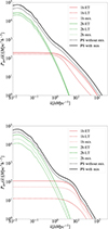Fig. 1. Galaxy power spectrum, evaluated at redshifts z = 0.001 (upper panel) and z = 2.0 (lower panel), broken down into the contributions from one-halo (1h) and two-halo (2h) terms, with (solid) and without (dashed) including the mixing terms between early-type (ET) and late-type (LT) galaxy populations. Red curves: 1h terms from ET (solid), LT (dashed) galaxies, and the mix (1h mix, dotted) between the two. Green curves: 2h terms from ET (solid), LT (dashed) galaxies and the mixing (2h mix, dotted) between the two. Black dashed curve: galaxy power spectrum without mixing terms between the two galaxy populations (PS without mix). Black solid curve: galaxy power spectrum with mixing terms (PS with mix).

3. The cosmic infrared background emission

The halo model provides information about the spatial distribution of galaxies but says nothing about their emission. In this section, we take the predictions of the halo model on how galaxies are distributed within dark matter halos and add modeling of the galaxies emission to present a physical description of the Cosmic Infrared Background (CIB) power spectrum. The key quantity that encapsulates the information on how galaxies emit as a function of redshift is the emissivity function, describing the redshift distribution of the cumulative flux density of sources below a threshold related to each experiment, i.e. the flux cut⁴$S_{\nu }^{\lim }$, and defined as

$$\begin{array}{c}\hfill j_{\nu }(z)={\displaystyle {\int }_0^{S_{\nu }^{\text{lim}}}}\frac{{\text{d}}^{3}N(S_{\nu },z)}{\text{d}{S}_{\nu }\text{d}z\text{d}\mathrm{\Omega }}{S}_{\nu }\text{d}{S}_{\nu }.\end{array}$$(35)

Here $\frac{{\mathrm{d}}^{3}N(S_{\nu },z)}{\mathrm{d}{S}_{\nu }\mathrm{d}z\mathrm{d}\mathrm{\Omega }}$ is the surface density of sources per unit flux density and redshift interval:

$$\begin{array}{c}\hfill \frac{{\text{d}}^{3}N(S_{\nu },z)}{\text{d}{S}_{\nu }\text{d}z\text{d}\mathrm{\Omega }}=\frac{\mathrm{\Phi }(log{L}_{\nu \prime },z)}{L_{\nu \prime }ln10}\frac{\text{d}{L}_{\nu \prime }}{\text{d}{S}_{\nu }}\frac{\text{d}V}{\text{d}z\text{d}\mathrm{\Omega }},\end{array}$$(36)

where ν′ and L_ν′ are the observed frequency and luminosity, $\frac{\mathrm{d}V}{\mathrm{d}z\mathrm{d}\mathrm{\Omega }}$ is the comoving volume per unit solid angle and Φ(log L_ν, z) is the luminosity function (LF), which quantifies the number of galaxies per unit volume with luminosity between L and $L+\mathrm{d}L$. The observed dichotomy in the galaxy populations enters when modeling the luminosity functions. ET and LT galaxies not only show different clustering properties, but also different emission properties. For this reason, in this work we adopt the hybrid approach, firstly introduced by C13, to model the emissions of the two galaxy populations.

From N-body simulations, ET galaxies are expected to populate more massive dark matter halos (Wang et al. 2011), for which it is easier to model the evolution. In fact, it is possible to extract an analytic model for the bolometric LF⁵ of ET galaxies, obtained as a convolution of the halo formation rate, $\mathrm{d}n/\mathrm{d}{t}_{\mathrm{vir}}$, with the galaxy luminosity distribution, P(log L, z) (see C13 for the complete overview of the model). To obtain the expression for the halo formation rate, we explicitly write $\mathrm{d}n$ from Eq. (8) as

$$\begin{array}{c}\hfill \text{d}n=\frac{\overline{\rho }}{m^2}\nu f(\nu )\frac{\text{d}ln\nu }{\text{d}lnm}\text{d}m,\end{array}$$(37)

and the halo formation rate, $\mathrm{d}n/\mathrm{d}{t}_{\mathrm{vir}}$, has been evaluated as:

$$\begin{array}{c}\hfill \frac{\text{d}n}{\text{d}{t}_{\text{vir}}}=\text{d}n\frac{\text{d}ln(\nu f(\nu ))}{\text{d}{t}_{\text{vir}}}·\end{array}$$(38)

The galaxy luminosity distribution is evaluated assuming a log-normal distribution, so that

$$\begin{array}{c}\hfill P(logL|log\overline{L})\text{d}logL=\frac{exp\{-{log}^2(L/\overline{L})/2{\sigma }^2\}}{\sqrt{2\pi {\sigma }^2}}\text{d}logL,\end{array}$$(39)

where $\overline{L}$ and σ are the mean luminosity and the dispersion of the distribution, respectively. The bolometric LF for the ET galaxies is then obtained as

$$\begin{array}{c}\hfill \mathrm{\Phi }(logL,z)={\displaystyle {\int }_{M_{\text{vir}}^{\text{min}}}^{M_{\text{vir}}^{\text{max}}}}\text{d}{M}_{\text{vir}}{\displaystyle {\int }_{z_{\text{vir}}^{\text{min}}}^{z_{\text{vir}}^{\text{max}}}}\text{d}{z}_{\text{vir}}|\frac{\text{d}{t}_{\text{vir}}}{\text{d}{z}_{\text{vir}}}|\frac{\text{d}n}{\text{d}{t}_{\text{vir}}}P(logL,z).\end{array}$$(40)

Late-type galaxies are expected to populate less massive dark matter halos, which more likely merge with other low-mass dark matter halos. This makes the modeling more challenging (Lapi & Cavaliere 2011), and for this reason LT galaxies require an empirical parameterization of their bolometric LF (see Saunders et al. 1990):

$$\begin{array}{c}\hfill \mathrm{\Phi }(logL,z)={\mathrm{\Phi }}^{\ast }(\frac{L}{L^{\ast }}{)}^{1-\alpha }exp\{-\frac{{log}^2(1+L/L^{\ast })}{2{\sigma }^2}\},\end{array}$$(41)

where Φ^* and L^* are the characteristic density and luminosity, respectively, α is the slope in the low-luminosity regime and σ is the dispersion of the galaxy population (see Table 1 of C13 for the values of this parameters).

The CIB emission is composed of two different components: a clustering term, describing the galaxy overdensities in the background tracing the dark matter distribution, and a shot noise term, describing the contribution of a diffuse background of unresolved sources.

To compute the clustering term of the CIB power spectrum we integrate the emissivity function, j_ν(z), describing how galaxies emit (Eq. 35), together with the non-linear galaxy power spectrum from the halo model formalism (Eq. 28):

$$\begin{array}{c}\hfill C_{\ell ,\nu \times \nu \prime }^{\text{clust}}={\displaystyle \int \frac{\text{d}z}{{\chi }^2}}\frac{\text{d}z}{\text{d}\chi }{j}_{\nu }(z)j_{\nu \prime }(z)P_{\text{gal}}(k=\ell /\chi ,z).\end{array}$$(42)

As mentioned above the non-linear galaxy power spectrum that enters in Eq. (42) includes three main contributions coming from ET galaxies, LT galaxies and the mixing among the two populations:

$$\begin{array}{c}\hfill P_{\text{gal}}(k)=P_{\text{gal}}^{\text{ET}}(k)+P_{\text{gal}}^{\text{LT}}(k)+P_{\text{gal}}^{\text{mix}}(k).\end{array}$$(43)

The emissivity functions in Eq. (42) account for the contributions coming from both galaxy populations,

$$\begin{array}{c}\hfill j_{\nu }(z)=j_{\nu }^{\text{ET}}(z)+j_{\nu }^{\text{LT}}(z).\end{array}$$(44)

When taking the product j_ν(z)j_ν′(z) in Eq. (42), we found

$$\begin{array}{c}\hfill \begin{array}{cc}\hfill j_{\nu }(z)j_{\nu \prime }(z)& =j_{\nu }^{\text{ET}}(z)j_{\nu \prime }^{\text{ET}}(z)+j_{\nu }^{\text{LT}}(z)j_{\nu \prime }^{\text{LT}}(z)\hfill \\ \hfill & +(j_{\nu }^{\text{ET}}(z)j_{\nu \prime }^{\text{LT}}(z)+j_{\nu }^{\text{LT}}(z)j_{\nu \prime }^{\text{ET}}(z)).\hfill \end{array}\end{array}$$(45)

In summary, we arrive to a clustering term of the CIB power spectrum composed of three terms:

$$\begin{array}{c}\hfill C_{\ell ,\nu \times \nu \prime }^{\text{clust}}=C_{\ell ,\nu \times \nu \prime }^{\text{ET,clust}}+C_{\ell ,\nu \times \nu \prime }^{\text{LT,clust}}+C_{\ell ,\nu \times \nu \prime }^{\text{mix,clust}}.\end{array}$$(46)

We expect that for z < 1, ET galaxies become quiescent, and therefore no longer contribute to the CIB power spectrum. This information is encapsulated in the emissivity functions, j_ν^ET/LT, which are truncated at z ∼ 1 for ET galaxies. The shape of the emissivity function for ET galaxies inherently accounts for their quiescence below a certain redshift, without requiring any additional parameters.

The shot noise (SN) component of the CIB power spectrum is obtained integrating the contribution of sources falling below the flux cut, $S_{\nu }^{\lim }$, of a given frequency channel and a given experiment:

$$\begin{array}{c}\hfill C_{\ell ,\nu }^{\mathrm{SN}}={\displaystyle {\int }_0^{S_{\nu }^{\text{lim}}}{S}_{\nu }^2}\frac{{\text{d}}^{2}N(S_{\nu })}{\text{d}{S}_{\nu }\text{d}\mathrm{\Omega }}\text{d}{S}_{\nu },\end{array}$$(47)

where ${\mathrm{d}}^{2}N(S_{\nu })/\mathrm{d}{S}_{\nu }\mathrm{d}\mathrm{\Omega }$ is obtained integrating Eq. (36) over redshift, and represents the differential number counts. The shot noise term is independent of the angular scale, thus representing a flat contribution to the CIB power spectrum when expressed in C_ℓs. In this study, the shot noise level for a specific frequency channel ν, SN_ν, is modeled as

$$\begin{array}{c}\hfill C_{\ell ,\nu \times \nu \prime }^{\mathrm{SN}}={\mathcal{C}}_{\nu \times \nu \prime }\sqrt{{\mathrm{SN}}_{\nu }\times {\mathrm{SN}}_{\nu \prime }},\end{array}$$(48)

where 𝒞_{ν1 × ν2} accounts for the possible correlation between emissions at different frequencies.

Finally, the CIB power spectrum is given by the sum of clustering and shot noise terms:

$$\begin{array}{c}\hfill C_{\ell ,\nu \times \nu \prime }^{\mathrm{CIB}}=C_{\ell ,\nu \times \nu \prime }^{\text{clust}}+C_{\ell ,\nu \times \nu \prime }^{\mathrm{SN}}.\end{array}$$(49)

Figure 2 shows the model predictions for the CIB power spectrum (black curve), highlighting the different contributions coming from ET (blue), LT (green), mixing terms (orange) and shot noise (red). This is plotted for two different frequency combinations: 217 × 217 GHz (dashed curves) and 1200 × 1200 GHz (solid curves), taking the two extremes of the data sets which we will use in Sect. 5. The figure shows that the LT galaxies dominate at higher frequencies (comparing the solid and dashed green curves) and that large angular scales (low multipoles) are dominated by the clustering terms, while the contribution coming from the constant shot noise term becomes more and more relevant as we move to higher multipoles, i.e. smaller angular scales.

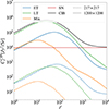Fig. 2. Different contributions to the CIB power spectrum as predicted by our model, for two different frequency combinations: 217 × 217 GHz (dashed curves), and 1200 × 1200 GHz (solid curves). In both cases, the contribution from early-type (ET) galaxies is in blue, for late-type (LT) galaxies in green and the mixing between the two galaxy populations in orange. The shot noise term is the flat contribution shown in red. The total CIB power spectrum (Eq. 49) is shown in black. The values of the model parameters used to produce these curves are: $log(M_{\min }^{\mathrm{ET}}/{\mathrm{M}}_{\odot }{h}^{-1})=12.07$, $log(M_{\min }^{\mathrm{LT}}/{\mathrm{M}}_{\odot }{h}^{-1})=10.85$, ${\alpha }_{\mathrm{ET}}=1$, ${\alpha }_{\mathrm{LT}}=1$, SN217 = 16 and SN1200 = 9833.

4. Dataset

To constrain the parameters describing the clustering properties of the two galaxy populations, we fit our model to three data sets: the CIB power spectrum measurements from Planck Collaboration XXX (2014) (denoted as P14 in this work), the CIB power spectrum obtained from a re-analysis of Planck data by Lenz et al. (2019) (hereafter L19), and the angular power spectra from Herschel-SPIRE data presented by Viero et al. (2019) (hereafter V19).

4.1. Planck data

P14 presented measurements of the CIB power spectrum over five frequencies, using a total area of 2240 deg² and spanning 143–857 GHz. The flux density cuts applied at the map level are S_ν^lim= 350, 225, 315, 350, 710 mJy for the 143, 217, 353, 545, 857 GHz frequency channels, respectively (see Table 1 of P14). In this study, we use ten CIB power spectra from P14, selecting only four frequency channels (217, 353, 545 and 857 GHz). In analogy with P14, we do not include the 143 GHz measurements for model fits since this channel has significant CMB signal contaminating the CIB (the CMB power spectrum at ℓ = 100 is ∼5000 higher than that of the CIB). This can be overcome implementing large corrections in the analysis to remove the CMB, but neither P14 nor this work attempt to do this.

The P14 data set covers the multipole range from ℓ = 150 to ℓ = 2500, binned using a logarithmic binning, Δℓ/ℓ = 0.3. Across this range, P14 provides 8 data points for each CIB frequency auto- and cross-spectrum, resulting in a total of 80 data points in the data set available for the model fit that is described in Sect. 5. The error bars associated to each point account for both cosmic variance and instrumental noise. Since P14 data come without a covariance matrix, we conduct our analysis building a diagonal covariance matrix from the spectra error bars and therefore neglecting possible correlations between different multipoles.

Data from Planck have been calibrated in two different ways, depending on the frequency channel. Specifically, the calibrator for the 217 and 353 GHz channels is the CMB orbital dipole, which boasts superior accuracy, while the 545 and 857 GHz channels are calibrated using planetary measurements. The calibration method generates a frequency-dependent uncertainty, with all values reported in Table 6 of Planck Collaboration VIII (2016) and used in later sections when fitting the spectra. Additionally, updates to the calibrations were introduced between the first and the second Planck Public Releases, i.e. PR1 and PR2. The CIB spectra are from PR1 and to account for these calibration updates here we correct them with

$$\begin{array}{c}\hfill C_{\ell ,{\nu }_1\times {\nu }_2}^{\mathrm{CIB}}=\frac{C_{\ell ,{\nu }_1\times {\nu }_2}^{\mathrm{CIB},PR1}}{{\mathrm{corr}}_{{\nu }_1}\times {\mathrm{corr}}_{{\nu }_2}}·\end{array}$$(50)

C_{ℓ, ν1 × ν2}^CIB represents the calibration-corrected data fed in input to the fit, C_{ℓ, ν1 × ν2}^CIB, PR1 are the original CIB power spectra presented in P14 and corr_νi are the calibration corrections for each frequency, as detailed in Planck Collaboration VIII (2016), and corresponding to 0.991, 0.997, 1.018, 1.033 for the 217, 353, 545 and 857 GHz frequency channels, respectively.

As detailed in the next section, to compare the model predictions with the data we also need to apply color corrections. Specifically, P14 analysis computes the color corrections for each frequency channel using the CIB SED from Bethermin et al. (2012), ending up with color-correction factors of 1.119, 1.097, 1.068 and 0.995 for the 217, 353, 545 and 857 GHz frequency channels, respectively.

4.2. Lenz data

The second data set explored in this study is L19 (Lenz et al. 2019), which provides six CIB power spectra using the 353, 545 and 857 GHz Planck maps – L19 excludes both 143 and 217 GHz channels on the basis of CMB contamination. As described in their measurements paper, the authors of L19 employed a method based on neutral atomic hydrogen data to remove Galactic dust from the Planck intensity maps. This procedure allows to extract the CIB power spectra down to lower multipoles compared to P14, reaching ℓ ∼ 75 (extending the P14 CIB power spectra starting from ℓ ∼ 150). L19 CIB data are also presented with a different and less aggressive binning scheme than the one of P14. Specifically, the authors apply a linear binning, including 64 multipoles in each bin and resulting in a data set with a total of 186 data points.

From the L19 dataset, we decide to exclude the first three bandpowers of each spectrum. We do this for two reasons: to better allow for a straightforward comparison with P14 data, and noting that the P14 data exhibit more power at lower multipoles compared to the L19 bandpowers (see Fig. 11 of L19). This could be due to a more aggressive dust cleaning procedure adopted in L19 but the consistency of the two data sets is beyond the scope of this work and not fully addressed in other literature for us to trust those additional bandpowers. We explore a few assumptions, including an investigation on the impact of the dust contamination in the L19 analysis in Appendix B.

As for P14, we apply to the L19 data set color corrections and the calibration factors, using the same values quoted in the previous subsection.

Similarly to P14, L19 spectra have been released without a covariance matrix. Once again, here we build a diagonal covariance between bandpowers, neglecting possible correlations between bands – we explore more this assumption in Appendix B.

4.3. SPIRE data

The third data set used in this work is the V19 CIB measurement from Herschel-SPIRE observations⁶. This covers higher frequencies and multipoles than those covered by the Planck data, providing complementary information on CIB physics. In particular, the higher angular resolution is expected to better probe the multipole region dominated by shot noise contribution, as opposed to the Planck scales which are more sensitive to the clustering term.

SPIRE observations approached the THz regime, covering 600, 857 and 1200 GHz from 90 deg². V19 applied a common flux density cut to the three frequency bands of S_ν^lim = 300 mJy. The CIB spectra span multipoles from ℓ = 600 to ℓ = 11 000. Following the binning scheme of Amblard et al. (2011), the bandpowers are linearly binned for ℓ < 1950, and for higher multipoles a logarithmic binning with Δℓ/ℓ = 720 is applied. In total, this data set consists of 132 data points.

The maps are calibrated with uncertainty of 5% for each frequency channel. The color corrections needed at 600, 857 and 1200 GHz are 0.9988, 0.9929 and 0.9957, respectively (Lagache et al. 2003).

SPIRE spectra are accompanied by a covariance matrix which is, however, not well defined⁷. In analogy with other studies (see e.g., Maniyar et al. 2021) to overcome issues with the available covariance, we revert to assuming uncorrelated error bars also for V19 data, using a simple diagonal covariance matrix.

5. Results

Here we bring together the full model described in Sect. 3 and the three data sets in Sect. 4. We explore the model against the multi-frequency, multi-scale observations from Planck and Herschel-SPIRE individually. We discuss our results in the context of previous literature findings, and show that even this extended, two-population model – built to capture an extended frequency range – is not able to solve a tension between P14 and V19 CIB measurements which was reported in Maniyar et al. (2021) with a single-population model. This prevents us from achieving a joint fit using both data sets.

To compare the predictions of the model to the observed data, we correct the theory to account for instrument-specific corrections as follows:

$$\begin{array}{c}\hfill C_{\ell ,{\nu }_1\times {\nu }_2}^{\mathrm{CIB},\text{data}}={\mathcal{A}}_{{\nu }_{1}x{\nu }_2}\times c{c}_{{\nu }_1}\times c{c}_{{\nu }_2}\times C_{\ell ,{\nu }_1\times {\nu }_2}^{\mathrm{CIB},\text{model}}.\end{array}$$(51)

Here, $C_{\ell ,{\nu }_1\times {\nu }_2}^{\mathrm{CIB},\mathrm{model}}$ is the CIB power spectrum as predicted by the model ; ${\mathcal{A}}_{{\nu }_1\times {\nu }_2}=\sqrt{f_{\mathrm{cal}}^{{\nu }_1}\times f_{\mathrm{cal}}^{{\nu }_2}}$ accounts for the absolute calibration uncertainties, i.e. $f_{\mathrm{cal}}^{{\nu }_i}$ for each different frequency channels; cc_νi is the color correction per frequency channel.

To explore the parameters of the model, we perform a Monte Carlo Markov Chain (MCMC) analysis by making use of the emcee ensemble sampler (Foreman-Mackey et al. 2013). The multi-dimensional parameter space is explored sampling a Gaussian likelihood:

$$\begin{array}{c}\hfill {\displaystyle log\mathcal{L}(C_{\ell }^{\text{data}}|C_{\ell }^{\text{model}})\propto -\frac{1}{2}{\displaystyle \sum _{\ell }}\frac{(C_{\ell }^{\text{data}}-C_{\ell }^{\text{model}}{)}^2}{{\sigma }_{\ell }^2},}\end{array}$$(52)

where σ_ℓ² represents the error bars associated to the points of each data set (i.e., representing a diagonal covariance matrix for all the three data sets).

The analysis has taken into consideration different scenarios and the numbers of fixed or varied model parameters has been set accordingly in each case as we describe below and in the individual subsections.

We perform our analyses covering two scenarios for the shot noise term:

• In one case, we assume maximal correlation between the shot noise contributions, with the correlation coefficients in Eq. (48) all set to 1.

• In another case, the correlation coefficients are treated as free parameters in the MCMC analysis.

The data considered in this work are able to constrain, with different degrees of sensitivity, the clustering parameters for both the early and the late galaxy populations, i.e., $M_{\min }^{\mathrm{ET}}$, ${\alpha }_{\mathrm{ET}}$, $M_{\min }^{\mathrm{LT}}$ and ${\alpha }_{\mathrm{LT}}$; the shot noise levels for the considered frequency channels, SN_νi; and the calibration factors, $f_{\mathrm{cal}}^{{\nu }_i}$. However, the data sets covering Planck frequencies and multipole ranges are not able to constrain the ${\alpha }_{\mathrm{ET}}$ clustering parameter (see Appendix A.1.) which we then fix to 1 for P14 and L19. On the other hand, as we show later, all data sets considered in this work can constrain ${\alpha }_{\mathrm{LT}}$ (either unconstrained or only weakly constrained in previous works) and this parameter is therefore always varied in our runs.

The choice of the prior distributions assigned to the free parameters, and the discussion and implications of the results from the individual model fits are discussed in the following sub-sections.

5.1. P14 data analysis

For P14 we sample 10 and 16 free parameters for the two scenarios, respectively, with prior ranges listed in the second column of Table 2. As mentioned above, expecting no constraining power from Planck , in the baseline case we fix ${\alpha }_{\mathrm{ET}}=1$ (and explore its variation in Appendix A.1.). We vary the calibration factors with a Gaussian prior centered on 1 and with errors taken as twice the uncertainty in Table 6 of Planck Collaboration VIII (2016), except for the calibration factor at 217 GHz which we fix to f_cal²¹⁷ = 1⁸. The clustering parameters and the shot noise levels are sampled from uniform distributions. When correlation coefficients are treated as free parameters, these are also sampled from uniform prior distributions.

Results (1σ confidence level) for the two model scenarios with fixed/varied correlations are reported in the third and the fourth columns of Table 2. We obtain χ² = 81 with 70 degrees of freedom when fixing the correlation coefficients, and χ² = 45 when the correlation coefficients are free to vary (when the number of degrees of freedom is 64), with Probability To Exceed (PTE) of 17.9% and 96.9% for the two cases, respectively. We show how the best-fit model compares with the ten P14 CIB spectra in Fig. 3.

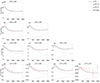Fig. 3. Comparison between P14 data and the model predictions obtained with the best-fit parameters in Table 2. The CIB power spectrum, the clustering term and the shot noise term predicted by the model are represented with the solid black, the dashed gray and the dot-dashed gray curves, respectively. P14 data with their error bars are represented in red.

In Fig. 4, we show the 1-dimensional posterior distributions and the 2-dimensional correlations (at 68 and 95% confidence) of the clustering parameters for the two scenarios considered in this work. The two cases are in good agreement, and as expected we recover larger constraints for some parameters due to the higher number of degrees of freedom in the MCMC when leaving correlations free to vary. The relative impact seen here on the best-fit values for the minimum mass of the ET and LT galaxies is likely due to the fact that, within the multipole range probed by P14 data, the contribution to the CIB power spectrum from clustering dominates, while the shot noise is expected to dominate at smaller angular scales. Therefore, the different treatment of the shot noise levels does not have a significant impact on the clustering parameters. Motivated by the results found on the L19 data set (see next section), we re-run the analysis removing the spectra involving 217 GHz and note much closer agreements between the two scenarios as shown in Fig. 5. To understand this we need to look at the full parameter space explored by the fit. We find a tension in the two scenarios for the value of the shot noise level of the 217 GHz frequency channel, shown in Fig. 6. Specifically, we obtain a value for the shot noise level which is higher in the case with free correlations than in the case with fixed correlations at ∼4σ level. We also see that the correlation coefficients involving the 217 GHz frequency channel, i.e., 𝒞_217 × i with i = 353, 545, 857 (see fourth column of Table 2), are significantly lower than unity. We explain this behavior by noting the degeneracy between the shot noise level and the correlation coefficients at 217 GHz (see Fig. 6), which P14 data are not able to break. Specifically, they are anti-correlated, meaning that a shift of the shot noise level toward a lower value, closer to the one obtained in the first scenario, leads to higher values of the 𝒞_217 × i.

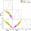Fig. 4. Posterior probability distributions of the clustering parameters for the two scenarios where the correlations for the shot noise are fixed to unity (in purple) and where they are free parameters in the fit (in green). The posterior distributions for the two cases are in agreement, exploring the same regions of the parameter space. We fix ${\alpha }_{\mathrm{ET}}=1$.

Fig. 5. Same as Fig. 4 excluding the 217 GHz frequency channel.

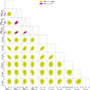Fig. 6. Posterior probability distributions of the shot noise levels for the scenario where the correlation coefficients are fixed to unity (in purple), and posterior probability distributions for the shot noise levels and the correlation coefficients for the scenario where the latter are free to vary (in green). This figure highlights the movement in the 217 GHz shot noise and shows the degeneracies with parameters characterizing the spectra including at least one leg of the 217 GHz channel.

When comparing our results with other literature findings, we note significant deviations between the values for the minimum masses of both galaxy populations extracted here with those found in the literature, more evident for the ET galaxies. Specifically, we find the minimum mass, $log(M_{\min }^{\mathrm{ET}}/{\mathrm{M}}_{\odot }{h}^{-1})$, to be lower than previously reported values (see Table 1). In particular, when comparing the value we obtain when fixing the correlation coefficients for the shot noise to unity, $log(M_{\min }^{\mathrm{ET}}/{\mathrm{M}}_{\odot }{h}^{-1})=11.{45}_{-0.13}^{+0.16}$, with the ones of C13, $log(M_{\min }^{\mathrm{ET}}/{\mathrm{M}}_{\odot }{h}^{-1})=12.{00}_{-0.04}^{+0.04}$, and X12, $log(M_{\min }^{\mathrm{ET}}/{\mathrm{M}}_{\odot }{h}^{-1})=12.{09}_{-0.06}^{+0.06}$, we find a tension at the level of ∼4σ. In contrast, our analysis shows a higher value of the minimum mass for LT galaxies than the expected value found in C13 of $log(M_{\min }^{\mathrm{LT}}/{\mathrm{M}}_{\odot }{h}^{-1})=10.85\pm 0.06$, but it is still compatible with the current constraint within ∼1σ. This discrepancy raises a critical point as far as the model is concerned: our results suggest that the minimum mass for ET galaxies is not higher than that for LT, contrary to prior assumptions. We speculate that this inconsistency may stem from the limited frequency and multipole ranges covered by P14 data. These ranges may not be sufficiently wide to effectively distinguish between the contributions of the two galaxy populations to the CIB spectrum, and, consequently, brake the degeneracies among all the three clustering parameters (see Fig. 4). Concerning ${\alpha }_{\mathrm{LT}}$, as already mentioned, previous analyses only considered it fixed to unity. Here, ${\alpha }_{\mathrm{LT}}$ is a free parameter of the model fit and is constrained at the best fit values of ${\alpha }_{\mathrm{LT}}=1.{337}_{-0.072}^{+0.063}$ and ${\alpha }_{\mathrm{LT}}=1.{436}_{-0.067}^{+0.075}$ for the case where the correlation coefficients are fixed and free to vary, respectively.

We now comment on the shot-noise correlation coefficients, in the scenario where they are free to vary (fourth column of Table 2). To ease the comparison with previous Planck analyses, we also report in Table 3 the values of the correlation coefficients extrapolated from Table 6 of P14, as

$$\begin{array}{c}\hfill {\mathcal{C}}_{{\nu }_1\times {\nu }_2}=\frac{C_{\ell ,{\nu }_1\times {\nu }_2}^{\text{Planck}}}{\sqrt{C_{\ell ,{\nu }_1\times {\nu }_1}^{\text{Planck}}{C}_{\ell ,{\nu }_2\times {\nu }_2}^{\text{Planck}}}},\text{with}{\nu }_1\ne {\nu }_2,\end{array}$$(53)

where $C_{\ell ,{\nu }_1\times {\nu }_2}^{\mathrm{Planck}}$ represent the entries of Table 6 of P14. We observe that the correlation coefficients involving the 217 GHz frequency channel, 𝒞_217 × i with i = 353, 545, 857, are always lower than the values reported in Table 3, even though they are still compatible within ∼2σ. On the other hand, the remaining correlation coefficients are compatible with the values in Table 3 within ∼1σ. The observed low correlation coefficients are likely due to non-trivial degeneracies between the free parameters of the model, which the specific data are not able to efficiently break. In other words, the number of free parameters for this second scenario is too high and the model overfits the data, and this is confirmed by the low χ² obtained in this scenario (χ² = 45).

5.2. L19 data analysis

In this section, we present the analysis of the L19 dataset. We note that, as explained in more details later, our model fits to L19 for both scenarios of correlations result in a poor χ². We, therefore, do not attempt to interpret the goodness of the fit to this data set and present results in this section only as a qualitative outcome.

The choice of the free parameters in the model fit and their prior distributions mirror what was described in the previous section and are listed in the first and second column of Table 4, respectively. As done for the analysis of P14 data, ${\alpha }_{\mathrm{ET}}$ is fixed to unity, and the priors for the calibration factors of the 353, 545, and 857 GHz channels are based on Planck uncertainties.

In Table 4, we also report the 1σ confidence level results in both the scenarios of fixed (third column) and variable (fourth column) shot noise correlation coefficients. In Fig. 7, we show the posterior distributions of the clustering parameters for the two scenarios of shot noise correlation coefficients fixed to unity (in purple), and free-to-vary correlation (in green). The results show perfect agreement between the two scenarios, with only a minor broadening of the distributions in the case of increased degrees of freedom in the fit. Specifically, we note that the posterior distributions deviate much less than those of P14 seen in Fig. 4, confirming that the exclusion of the 217 GHz frequency channel – not included at all in the L19 data set – makes the results of the fits more stable among the two scenarios.

Fig. 7. Same as Fig. 4 but for the L19 CIB dataset.

The model fits to the L19 data result in poor goodness-of-the-fit metrics, in particular in exceedingly high χ² values (specifically we obtained a χ² of 655 and 650 for 159 and 156 degrees of freedom, respectively). However, we cannot definitely conclude that this is caused by deficits in the model. Appendix B is devoted to a detailed and closer examination of the L19 dataset; we show there how a smooth theory cannot meet the bandpowers as published, and that changing assumptions in the data set is also not enough to improve the χ² and that the qualitative results presented here remain valid.

Without focusing on the exact results from L19, in the following we do a qualitative exploration of how the posteriors compare to those of P14. The clustering parameters for the two scenarios explored in this study are shown in Figs. 8 and 9. The overlap between the two data sets is good (the largest shift is noted in the 1D posterior distribution of the minimum masses for the LT galaxies in Fig. 9, approaching a ∼3σ difference).

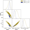Fig. 8. Comparison of the posterior distributions of the clustering parameters for P14 (dark yellow) and L19 (dark purple) data in the case in which the correlation coefficients of the shot noise are fixed to unity.

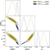Fig. 9. Same as Fig. 8 but for the case in which the correlation coefficients of the shot noise are free to vary.

5.3. Herschel-SPIRE data analysis

We now move to discuss the results from the V19 SPIRE dataset.

The model parameters and the prior distributions adopted in the analysis are reported in the first and second column of Table 5, respectively. Unlike the previous data sets, the SPIRE data allows to constrain the ${\alpha }_{\mathrm{ET}}$ clustering parameter. We therefore let it be free to vary along with the other clustering parameters. The calibration factors for the three frequency channels, $f_{\mathrm{cal}}^i$ with i = 600, 857, 1200, are varied with a Gaussian prior centered on 1 and a 1σ width determined as twice the calibration accuracy reported in Valtchanov (2017). As done for the P14 and L19 analyses, we consider two scenarios of fixed and free-to-vary shot-noise correlation coefficients.

The results of the model fit (68% confidence level) for the two cases under study are reported in the third and the fourth columns of Table 5. We obtain χ² = 101 for 122 degrees of freedom, when fixing the correlation coefficients for the shot noise, and χ² = 80 for the scenario where the correlation coefficients are free to vary and the number of degrees of freedom is 119. The spectra-model comparison is shown in Fig. 10, for the case where the correlation coefficients for the shot noise are fixed to unity across all the V19 spectra. Specifically, V19 data starts to be sensitive not only to the information coming from the clustering part, but also to the shot noise contribution. We find good agreement both in the multipole region where the clustering dominates and in the region when the shot noise dominates, at all frequencies.

Fig. 10. Same as Fig. 3 but for the V19 data set and using the best-fit parameters from Table 5.

Figure 11 shows the posterior distributions of the clustering parameters when fixing the correlation coefficients for the shot noise to unity (purple) and when letting them free to vary (green).

Fig. 11. Same as Fig. 4 but for the V19 CIB dataset.

The best-fit values which we obtain for the minimum mass of the ET galaxies are higher than those obtained in the analysis conducted on P14 data. They are also higher than the ones previously found in C13 and X12 (and reported in Table 1). Similarly, the minimum mass for LT galaxies in both scenarios explored in this work appears to be higher that the value found in C13 ($log(M_{\min }^{\mathrm{LT}}/{\mathrm{M}}_{\odot }{h}^{-1})=10.85\pm 0.06$), totalling a ∼4σ tension between our work and previous literature. This difference could be explained by the fact that we are exploring an extended model compared to C13 who fixed ${\alpha }_{\mathrm{LT}}=1$. In fact, from Fig. 11 we note that, due to the positive correlation between $log(M_{\min }^{\mathrm{LT}})$ and ${\alpha }_{\mathrm{LT}}$, values of ${\alpha }_{\mathrm{LT}}$ closer to unity will pull $log(M_{\min }^{\mathrm{LT}})$ toward lower values.

Our results also showcase the ability of V19 data to distinguish among the two galaxy populations and therefore their sensitivity to ${\alpha }_{\mathrm{ET}}$, which is unconstrained by Planck. The constraints on ${\alpha }_{\mathrm{ET}}$ are in agreement with semi-analytical models (Gao et al. 2004; Hansen et al. 2009), predicting ${\alpha }_{\mathrm{ET}}\le 1.0$. However, we note that these results are not in agreement with the estimated values of ${\alpha }_{\mathrm{ET}}=1.55\pm 0.05$ and ${\alpha }_{\mathrm{ET}}=1.81\pm 0.04$ found in C13 and X12, corresponding to a tension of ∼4σ and 5σ respectively. The discrepancy between our findings and those of C13 and X12 reduces when considering the correlation coefficients of the shot noise as free parameters. Specifically, the ${\alpha }_{\mathrm{ET}}$ clustering parameter in that scenario is compatible with the values of C13 and X12 within 1σ and 2σ, respectively. We can explain this better agreement looking at how the model parameters act on the spectra. The ${\alpha }_{\mathrm{ET}}$ clustering parameter (as well as ${\alpha }_{\mathrm{LT}}$) re-scale the overall power, similarly to calibration factors. From Table 5, we see that in the case of free correlations, the shot noise values change and carry with them the correlation factors which go low and reduce power in the spectra. This is then compensated by power added back in by higher clustering parameters. Concerning the spectral index of LT galaxies, a previous study conducted by C13 shows that ${\alpha }_{\mathrm{LT}}$ was only weakly constrained and therefore kept fixed at unity. Here we show that the V19 data are capable of constraining this parameter at ${\alpha }_{\mathrm{LT}}=1.253\pm 0.044$ and ${\alpha }_{\mathrm{LT}}=1.311\pm 0.071$ for the two scenarios.

Shot noise levels depend on the scenario under scrutiny. When assuming maximal correlation between frequencies (correlation coefficients fixed to unity), the shot noise values are a factor of ∼2 smaller than the levels predicted by the model of Bethermin et al. (2012) and reported in Table 4 of Lagache et al. (2020). Allowing shot noise correlation coefficients to vary, or in other words, giving more freedom to the model fit, leads the parameters to move toward values that are closer to the ones reported in the literature.

We conclude by commenting on the calibration factors. They are generally consistent with 1 within 1σ regardless of the treatment of the shot noise correlation coefficients. We only report a low value of the 1200 GHz factor $f_{\mathrm{cal}}^{1200}$, which deviates from 1 at 2σ in the case of free-to-vary correlations between shot noise levels. This may compensate for a lower value of the shot noise level at 1200 GHz with respect to the value found in the case of fixed shot-noise correlations.

5.4. P14 and V19 comparison

Given the general agreement between the posterior distributions of P14 and L19 shown in Sect. 5.2 and given the qualitative nature of our L19 results, in this section we compare the results between Planck and SPIRE data taking the P14 and V19 results.

Figures 12 and 13 show the posterior distributions of the clustering parameters for V19 (in dark blue) and P14 (in dark yellow) for the case in which the correlation coefficients of the shot noise are fixed to unity and the case in which they are free to vary, respectively. From the inspection of these figures, we note a tension between the two data sets in the best-fit values of the minimum mass of the ET galaxies, at the level of ∼5σ for both scenarios. We find better agreement for the $log(M_{\min }^{\mathrm{LT}}/{\mathrm{M}}_{\odot }{h}^{-1})$ and ${\alpha }_{\mathrm{LT}}$ clustering parameters. Specifically, the best-fit values for the minimum mass for LT galaxies from the two data sets are in agreement within ∼2σ when fixing the correlation coefficients, and ∼1σ for the case where the correlation coefficients are free to vary. Lastly, the best-fit values for the ${\alpha }_{\mathrm{LT}}$ clustering parameter are in agreement within ∼1σ for the two data sets and for both the scenarios explored in this study. We remind the reader that the P14 data do not allow to provide significant constraining power for α_ET, which is thus fixed to 1.

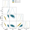Fig. 12. Comparison of the posterior distributions of the clustering parameters from P14 (dark yellow) and V19 (dark blue) data for the case in which the correlation coefficients of the shot noise are fixed to unity. The two posterior distributions are in tension, not exploring the same regions of the parameter space.

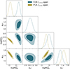Fig. 13. Same as Fig. 12 but for the case in which the correlation coefficients of the shot noise are free to vary in the analysis. The two data sets are still in tension.

We performed a number of tests to verify this comparison and to understand the impact of method and model assumptions on the agreement/disagreement. In particular, for P14 we tried excluding the 217 GHz frequency channel and fixing the ${\alpha }_{\mathrm{ET}}$ clustering parameter to values different from 1 (e.g. ${\alpha }_{\mathrm{ET}}=0.5$ and ${\alpha }_{\mathrm{ET}}=1.5$). For V19, we performed the MCMC fixing the ${\alpha }_{\mathrm{ET}}$ clustering parameter in order to recover the same setup used for P14. None of these tests improved the agreement between the two data sets. Given the tension between the two data sets, we do not perform a joint analysis. The tests we have done and the limited availability to compare overlapping scales do not allow us to clearly identify the source of the discrepancy between the data sets. The tension may equally point at inherent differences in the data sets or a failure in the ability of our model to capture the complexity of the physics under scrutiny (for example, we are not including the luminosity dependence of the HOD, as done in Viero et al. 2013). The analysis of independent data from other surveys may help shed light into this tension.

6. Conclusions and future perspectives

In this work, we applied a halo model formalism to derive a physically motivated model of the CIB emission. The model includes contributions to the CIB emission generated by two different types of galaxy populations, namely early-type (ET) and late-type (LT) galaxies, which show different halo distribution and emission characteristics. For the first time, the mixing terms between these populations has also been fully integrated into the calculations. In the model, we distinguish between a contribution from the clustering of matter to the CIB power spectrum (dominating at larger angular scales) and a shot noise contribution (dominating at smaller scales). We populate dark matter halos with two galaxy populations to explain two phenomena. Firstly, galaxy number counts exhibit a bimodal distribution suggesting different behaviors for different galaxies. Secondly, previous attempts to model the CIB power spectrum using a single galaxy population have failed to fit all data accurately. We compare our model against three state-of-the-art data sets – data from the official Planck release (P14), a reanalysis of Planck data by Lenz (L19), and data from Herschel-SPIRE (V19). The data sets have been chosen so to cover two observational regimes: lower frequency and lower multipole ranges (Planck); high-frequency, high-multipoles ranges (SPIRE). The two regimes map onto different sensitivities to the model parameters and contributions from galaxy populations. As we summarize below, despite our extension, the model still faces challenges in describing all these data sets.

We found that P14 data provide information on the clustering parameters. However, the frequency range probed with P14 is not wide enough to effectively distinguish between contributions from the two galaxy populations. Qualitatively, L19 data say the same story. The same does not apply to V19. In this case, the analysis allows to constrain the clustering parameters of both ET and LT galaxies.

When comparing the results from P14 and V19, we report – in agreement with previous analyses (see e.g., Maniyar et al. 2021) – a tension between the two data sets. This discrepancy is severe enough to prevent us from performing a joint fit. At this stage, we are unable to clearly pinpoint the source of this discrepancy, which might be due to either the data themselves or to model assumptions (or both). If we assume that the two-population model is a correct and complete description of all CIB emission, the difficulty in fitting the data may be due to e.g., other signals contaminating what we consider a CIB-only data set or a mistreatment of other experimental factors (such as beams or calibrations). In Appendix B (available at https://zenodo.org/records/13960802), we demonstrate how possible dust residuals affect the clustering parameters for the L19 dataset. Alternatively, if we take current data at face value and assume that they are a clean measurement of the CIB emission, the tension might indicate that our model is still incomplete. However, at present, there are no additional astrophysical signatures guiding us in refining the model further.

Our work also highlights that the results are highly dependent on the choices made in the analysis and on which priors and external information are imposed on the parameters. We provide a long list of tests in this paper but found limitations in the constraining power of the data sets at hand, we need new observations to be able to lock in further the model.

The tension observed between the low- and high-frequency/multipole range experiments suggests that surveys spanning wider frequency/angular scale coverage could help shed light on the current discrepancies, as well as advance our understanding of the physics of CIB emission.

The approach used here for the CIB can be extended to provide a physical description of the Sunyaev Zeldovich (SZ) effect. Furthermore, being CIB and SZ tracers of the same underlying matter distribution, the extension of the halo model approach to the SZ effect will also allow properly predict the correlation between the two tracers (building on other existing literature).

Data availability

Supplementary material and more detailed discussions are available at https://zenodo.org/records/13960802. Appendices A, B, and C contain the full triangle plots, showing the posterior distributions for all three data sets, along with a comparison of the model predictions with observational data. Appendix A.1 focuses on the results of the model fit to the P14 data, allowing the α_ET clustering parameter to vary freely. Appendix B.2 presents a series of tests on the L19 data set, analyzing the impact of the covariance matrix on the model fit and investigating potential dust contamination.

Finally, Appendix D provides an overview of the general structure of our code.

Acknowledgments

We thank Laura Salvati and Ian Harrison for useful discussions during the preparation of this work. We thank Abhishek Maniyar for valuable information about the halomodel_cib_tsz_cibxtsz code (Maniyar et al. 2021). GZ thanks the Cardiff University for hospitality during the finalization of the manuscript. We acknowledge the use of numpy (Harris et al. 2020), matplotlib (Hunter 2007) and getdist (Lewis 2019) software packages. We acknowledge the CINECA award under the ISCRA initiative, for the availability of high performance computing resources. EC acknowledges support from the European Research Council (ERC) under the European Union’s Horizon 2020 research and innovation programme (Grant agreement No. 849169). GZ and MG are funded by the European Union (ERC, RELiCS, project number 101116027). Views and opinions expressed are however those of the author(s) only and do not necessarily reflect those of the European Union or the European Research Council Executive Agency. Neither the European Union nor the granting authority can be held responsible for them. MG, GZ, CC, MG and LP acknowledge the financial support from the COSMOS network (www.cosmosnet.it) through the ASI (Italian Space Agency) Grants 2016-24-H.0 and 2016-24-H.1-2018.

References

All Tables

All Figures

Fig. 1. Galaxy power spectrum, evaluated at redshifts z = 0.001 (upper panel) and z = 2.0 (lower panel), broken down into the contributions from one-halo (1h) and two-halo (2h) terms, with (solid) and without (dashed) including the mixing terms between early-type (ET) and late-type (LT) galaxy populations. Red curves: 1h terms from ET (solid), LT (dashed) galaxies, and the mix (1h mix, dotted) between the two. Green curves: 2h terms from ET (solid), LT (dashed) galaxies and the mixing (2h mix, dotted) between the two. Black dashed curve: galaxy power spectrum without mixing terms between the two galaxy populations (PS without mix). Black solid curve: galaxy power spectrum with mixing terms (PS with mix).

In the text

Fig. 2. Different contributions to the CIB power spectrum as predicted by our model, for two different frequency combinations: 217 × 217 GHz (dashed curves), and 1200 × 1200 GHz (solid curves). In both cases, the contribution from early-type (ET) galaxies is in blue, for late-type (LT) galaxies in green and the mixing between the two galaxy populations in orange. The shot noise term is the flat contribution shown in red. The total CIB power spectrum (Eq. 49) is shown in black. The values of the model parameters used to produce these curves are: $log(M_{\min }^{\mathrm{ET}}/{\mathrm{M}}_{\odot }{h}^{-1})=12.07$, $log(M_{\min }^{\mathrm{LT}}/{\mathrm{M}}_{\odot }{h}^{-1})=10.85$, ${\alpha }_{\mathrm{ET}}=1$, ${\alpha }_{\mathrm{LT}}=1$, SN217 = 16 and SN1200 = 9833.

In the text

	Fig. 3. Comparison between P14 data and the model predictions obtained with the best-fit parameters in Table 2. The CIB power spectrum, the clustering term and the shot noise term predicted by the model are represented with the solid black, the dashed gray and the dot-dashed gray curves, respectively. P14 data with their error bars are represented in red.
In the text

	Fig. 4. Posterior probability distributions of the clustering parameters for the two scenarios where the correlations for the shot noise are fixed to unity (in purple) and where they are free parameters in the fit (in green). The posterior distributions for the two cases are in agreement, exploring the same regions of the parameter space. We fix ${\alpha }_{\mathrm{ET}}=1$.
In the text

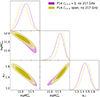	Fig. 5. Same as Fig. 4 excluding the 217 GHz frequency channel.
In the text

Fig. 6. Posterior probability distributions of the shot noise levels for the scenario where the correlation coefficients are fixed to unity (in purple), and posterior probability distributions for the shot noise levels and the correlation coefficients for the scenario where the latter are free to vary (in green). This figure highlights the movement in the 217 GHz shot noise and shows the degeneracies with parameters characterizing the spectra including at least one leg of the 217 GHz channel.

In the text

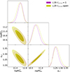	Fig. 7. Same as Fig. 4 but for the L19 CIB dataset.
In the text

	Fig. 8. Comparison of the posterior distributions of the clustering parameters for P14 (dark yellow) and L19 (dark purple) data in the case in which the correlation coefficients of the shot noise are fixed to unity.
In the text

	Fig. 9. Same as Fig. 8 but for the case in which the correlation coefficients of the shot noise are free to vary.
In the text

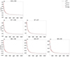	Fig. 10. Same as Fig. 3 but for the V19 data set and using the best-fit parameters from Table 5.
In the text

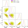	Fig. 11. Same as Fig. 4 but for the V19 CIB dataset.
In the text

	Fig. 12. Comparison of the posterior distributions of the clustering parameters from P14 (dark yellow) and V19 (dark blue) data for the case in which the correlation coefficients of the shot noise are fixed to unity. The two posterior distributions are in tension, not exploring the same regions of the parameter space.
In the text

	Fig. 13. Same as Fig. 12 but for the case in which the correlation coefficients of the shot noise are free to vary in the analysis. The two data sets are still in tension.
In the text

References

- Amblard, A., Cooray, A., Serra, P., et al. 2011, Nature, 470, 510 [NASA ADS] [CrossRef] [Google Scholar]
- Asgari, M., Mead, A. J., & Heymans, C. 2023, ArXiv e-prints [arXiv:2303.08752] [Google Scholar]
- Berlind, A. A., Weinberg, D. H., Benson, A. J., et al. 2003, ApJ, 593, 1 [NASA ADS] [CrossRef] [Google Scholar]
- Bethermin, M., Daddi, E., Magdis, G., et al. 2012, ApJ, 757, L23 [NASA ADS] [CrossRef] [Google Scholar]
- Bhattacharya, S., Heitmann, K., White, M., et al. 2011, ApJ, 732, 122 [NASA ADS] [CrossRef] [Google Scholar]
- Bocquet, S., Heitmann, K., Habib, S., et al. 2020, ApJ, 901, 5 [Google Scholar]
- Bond, J. R., Cole, S., Efstathiou, G., & Kaiser, N. 1991, ApJ, 379, 440 [NASA ADS] [CrossRef] [Google Scholar]
- Bullock, J. S., Kolatt, T. S., Sigad, Y., et al. 2001, MNRAS, 321, 559 [Google Scholar]
- Cai, Z.-Y., Lapi, A., Xia, J.-Q., et al. 2013, ApJ, 768, 21 [NASA ADS] [CrossRef] [Google Scholar]
- Child, H. L., Habib, S., Heitmann, K., et al. 2018, ApJ, 859, 55 [NASA ADS] [CrossRef] [Google Scholar]
- Cooray, A., & Sheth, R. K. 2002, Phys. Rep., 372, 1 [NASA ADS] [CrossRef] [Google Scholar]
- Correa, C. A., Wyithe, J. S. B., Schaye, J., & Duffy, A. R. 2015, MNRAS, 452, 1217 [CrossRef] [Google Scholar]
- Courtin, J., Rasera, Y., Alimi, J. M., et al. 2011, MNRAS, 410, 1911 [NASA ADS] [Google Scholar]
- Crocce, M., Fosalba, P., Castander, F. J., & Gaztanaga, E. 2010, MNRAS, 403, 1353 [NASA ADS] [CrossRef] [Google Scholar]
- Despali, G., Giocoli, C., Angulo, R. E., et al. 2016, MNRAS, 456, 2486 [NASA ADS] [CrossRef] [Google Scholar]
- Diemer, B., & Joyce, M. 2019, ApJ, 871, 168 [NASA ADS] [CrossRef] [Google Scholar]
- Diemer, B., & Kravtsov, A. V. 2015, ApJ, 799, 108 [Google Scholar]
- Duffy, A. R., Schaye, J., Kay, S. T., & Dalla Vecchia, C. 2008, MNRAS, 390, L64, [Erratum: Mon. Not. Roy. Astron. Soc. 415, L85 (2011)] [Google Scholar]
- Eales, S., Lilly, S., Gear, W., et al. 1999, ApJ, 515, 518 [NASA ADS] [CrossRef] [Google Scholar]
- Eke, V. R., Navarro, J. F., & Steinmetz, M. 2001, ApJ, 554, 114 [NASA ADS] [CrossRef] [Google Scholar]
- Fixsen, D. J., Cheng, E. S., Gales, J. M., et al. 1996, ApJ, 473, 576 [Google Scholar]
- Foreman-Mackey, D., Hogg, D. W., Lang, D., & Goodman, J. 2013, PASP, 125, 306 [Google Scholar]
- Gao, L., White, S. D. M., Jenkins, A., Stoehr, F., & Springel, V. 2004, MNRAS, 355, 819 [Google Scholar]
- Grossan, B., & Smoot, G. F. 2007, A&A, 474, 731 [NASA ADS] [CrossRef] [EDP Sciences] [Google Scholar]
- Hall, N. R., Keisler, R., Knox, L., et al. 2010, ApJ, 718, 632 [NASA ADS] [CrossRef] [Google Scholar]
- Hansen, S. M., Sheldon, E. S., Wechsler, R. H., & Koester, B. P. 2009, ApJ, 699, 1333 [NASA ADS] [CrossRef] [Google Scholar]
- Harris, C. R., Millman, K. J., van der Walt, S. J., et al. 2020, Nature, 585, 357 [NASA ADS] [CrossRef] [Google Scholar]
- Howlett, C., Lewis, A., Hall, A., & Challinor, A. 2012, JCAP, 1204, 027 [Google Scholar]
- Hughes, D. H., Serjeant, S., Dunlop, J., et al. 1998, Nature, 394, 241 [Google Scholar]
- Hunter, J. D. 2007, Comput. Sci. Eng., 9, 90 [NASA ADS] [CrossRef] [Google Scholar]
- Jenkins, A., Frenk, C. S., White, S. D. M., et al. 2001, MNRAS, 321, 372 [Google Scholar]
- Kwan, J., Bhattacharya, S., Heitmann, K., & Habib, S. 2013, ApJ, 768, 123 [NASA ADS] [CrossRef] [Google Scholar]
- Lagache, G., Dole, H., & Puget, J. L. 2003, MNRAS, 338, 555 [Google Scholar]
- Lagache, G., Bavouzet, N., Fernandez-Conde, N., et al. 2007, ApJ, 665, L89 [NASA ADS] [CrossRef] [Google Scholar]
- Lagache, G., Béthermin, M., Montier, L., Serra, P., & Tucci, M. 2020, A&A, 642, A232 [NASA ADS] [CrossRef] [EDP Sciences] [Google Scholar]
- Lapi, A., & Cavaliere, A. 2011, Adv. Astron., 2011, 903429 [CrossRef] [Google Scholar]
- Lenz, D., Doré, O., & Lagache, G. 2019, ApJ, 883, 75 [Google Scholar]
- Lewis, A. 2019, ArXiv e-prints [arXiv:1910.13970] [Google Scholar]
- Lewis, A., Challinor, A., & Lasenby, A. 2000, ApJ, 538, 473 [Google Scholar]
- Ludlow, A. D., Navarro, J. F., Angulo, R. E., et al. 2014, MNRAS, 441, 378 [NASA ADS] [CrossRef] [Google Scholar]
- Ludlow, A. D., Bose, S., Angulo, R. E., et al. 2016, MNRAS, 460, 1214 [Google Scholar]
- Maccio’, A. V., Dutton, A. A., & Bosch, F. C. v. d. 2008, MNRAS, 391, 1940 [CrossRef] [Google Scholar]
- Mak, D. S. Y., Challinor, A., Efstathiou, G., Lagache, G., & Lagache, G. 2017, MNRAS, 466, 286 [NASA ADS] [CrossRef] [Google Scholar]
- Maniyar, A. S., Béthermin, M., & Lagache, G. 2018, A&A, 614, A39 [NASA ADS] [CrossRef] [EDP Sciences] [Google Scholar]
- Maniyar, A. S., Béthermin, M., & Lagache, G. 2021, A&A, 645, A40 [NASA ADS] [CrossRef] [EDP Sciences] [Google Scholar]
- McClintock, T., Rozo, E., Becker, M. R., et al. 2019, ApJ, 872, 53 [NASA ADS] [CrossRef] [Google Scholar]
- Mo, H. J., & White, S. D. M. 1996, MNRAS, 282, 347 [Google Scholar]
- Murray, S. G., Diemer, B., Chen, Z., et al. 2021, Astron. Comput., 36, 100487 [NASA ADS] [CrossRef] [Google Scholar]
- Navarro, J. F., Frenk, C. S., & White, S. D. M. 1997, ApJ, 490, 493 [Google Scholar]
- Neto, A. F., Gao, L., Bett, P., et al. 2007, MNRAS, 381, 1450 [NASA ADS] [CrossRef] [Google Scholar]
- Okoli, C., & Afshordi, N. 2016, MNRAS, 456, 3068 [Google Scholar]
- Peacock, J. A. 2007, MNRAS, 379, 1067 [Google Scholar]
- Peacock, J. A., & Smith, R. E. 2000, MNRAS, 318, 1144 [Google Scholar]
- Planck Collaboration XVIII. 2011, A&A, 536, A18 [NASA ADS] [CrossRef] [EDP Sciences] [Google Scholar]
- Planck Collaboration XXX. 2014, A&A, 571, A30 [NASA ADS] [CrossRef] [EDP Sciences] [Google Scholar]
- Planck Collaboration VIII. 2016, A&A, 594, A8 [NASA ADS] [CrossRef] [EDP Sciences] [Google Scholar]
- Prada, F., Klypin, A. A., Cuesta, A. J., Betancort-Rijo, J. E., & Primack, J. 2012, MNRAS, 423, 3018 [NASA ADS] [CrossRef] [Google Scholar]
- Press, W. H., & Schechter, P. 1974, ApJ, 187, 425 [Google Scholar]
- Puget, J. L., Abergel, A., Bernard, J. P., et al. 1996, A&A, 308, L5 [Google Scholar]
- Reed, D., Bower, R., Frenk, C., Jenkins, A., & Theuns, T. 2007, MNRAS, 374, 2 [NASA ADS] [CrossRef] [Google Scholar]
- Saunders, W., Rowan-Robinson, M., Lawrence, A., et al. 1990, MNRAS, 242, 318 [Google Scholar]
- Scoccimarro, R., Sheth, R. K., Hui, L., & Jain, B. 2001, ApJ, 546, 20 [NASA ADS] [CrossRef] [Google Scholar]
- Seljak, U. 2000, MNRAS, 318, 203 [Google Scholar]
- Sheth, R. K., & Tormen, G. 1999, MNRAS, 308, 119 [Google Scholar]
- Smail, I., Ivison, R. J., & Blain, A. W. 1997, ApJ, 490, L5 [NASA ADS] [CrossRef] [Google Scholar]
- Tinker, J. L., & Wetzel, A. R. 2010, ApJ, 719, 88 [NASA ADS] [CrossRef] [Google Scholar]
- Tinker, J. L., Kravtsov, A. V., Klypin, A., et al. 2008, ApJ, 688, 709 [NASA ADS] [CrossRef] [Google Scholar]
- Tinker, J. L., Robertson, B. E., Kravtsov, A. V., et al. 2010a, ApJ, 724, 878 [NASA ADS] [CrossRef] [Google Scholar]
- Tinker, J. L., Wechsler, R. H., & Zheng, Z. 2010b, ApJ, 709, 67 [NASA ADS] [CrossRef] [Google Scholar]
- Valtchanov, I. E. 2017, SPIRE Handbook v3.1, Herschel Explanatory Supplement, Vol. IV, hERSCHEL-HSC-DOC-0798 [Google Scholar]
- Viero, M. P., Wang, L., Zemcov, M., et al. 2013, ApJ, 772, 77 [Google Scholar]
- Viero, M. P., Reichardt, C. L., Benson, B. A., et al. 2019, ApJ, 881, 96 [NASA ADS] [CrossRef] [Google Scholar]
- Wang, J., Navarro, J. F., Frenk, C. S., et al. 2011, MNRAS, 413, 1373 [NASA ADS] [CrossRef] [Google Scholar]
- Warren, M. S., Abazajian, K., Holz, D. E., & Teodoro, L. 2006, ApJ, 646, 881 [NASA ADS] [CrossRef] [Google Scholar]
- Watson, W. A., Iliev, I. T., D’Aloisio, A., et al. 2013, MNRAS, 433, 1230 [Google Scholar]
- Xia, J.-Q., Negrello, M., Lapi, A., et al. 2012, MNRAS, 422, 1324 [NASA ADS] [CrossRef] [Google Scholar]
- Zehavi, I., Zheng, Z., Weinberg, D. H., et al. 2005, ApJ, 630, 1 [Google Scholar]