| Issue |
A&A
Volume 692, December 2024
|
|
|---|---|---|
| Article Number | A26 | |
| Number of page(s) | 20 | |
| Section | Stellar structure and evolution | |
| DOI | https://doi.org/10.1051/0004-6361/202450805 | |
| Published online | 29 November 2024 | |
The fast rise of the unusual type IIL/IIb SN 2018ivc
1
INAF – Osservatorio Astronomico di Brera, Via E. Bianchi 46, I-23807 Merate (LC), Italy
2
INAF – Osservatorio Astronomico di Padova, Vicolo dell’Osservatorio 5, I-35122 Padova, Italy
3
Instituto de Astrofísica, Universidad Andres Bello, Fernandez Concha 700, Las Condes, 8320000 Santiago RM, Chile
4
Millennium Institute of Astrophysics (MAS), Nuncio Monseñor Sótero Sanz 100, Providencia, 8320000 Santiago RM, Chile
5
Instituto de Alta Investigación, Universidad de Tarapacá, Casilla 7D, Arica, Chile
6
Department of Astronomy, Kyoto University, Kitashirakawa-Oiwake-cho, Sakyo-ku, Kyoto 606-8502, Japan
7
National Astronomical Observatory of Japan, National Institutes of Natural Sciences, and Graduate Institute for Advanced Studies, SOKENDAI, 2-21-1 Osawa, Mitaka, Tokyo 181-8588, Japan
8
School of Physics and Astronomy, Monash University, Clayton, Victoria 3800, Australia
9
Department of Physics and Astronomy, University of Turku, FI-20014 Turku, Finland
10
Finnish Centre for Astronomy with ESO (FINCA), FI-20014 University of Turku, Finland
11
Instituto de Astrofísica de La Plata (IALP), CCT-CONICET-UNLP, Paseo del Bosque S/N, B1900FWA La Plata, Argentina
12
Facultad de Ciencias Astronómicas y Geofísicas, Universidad Nacional de La Plata, Paseo del Bosque S/N, B1900FWA La Plata, Argentina
13
Kavli Institute for the Physics and Mathematics of the Universe (WPI), The University of Tokyo, 5-1-5 Kashiwanoha, Kashiwa, Chiba 277-8583, Japan
14
European Southern Observatory, Alonso de Córdova 3107, Casilla 19, 8320000 Santiago, Chile
15
School of Physics, O’Brien Centre for Science North, University College Dublin, Belfield, Dublin 4, Ireland
16
Astronomical Observatory, University of Warsaw, Al. Ujazdowskie 4, 00-478 Warszawa, Poland
17
Astrophysics Research Centre, School of Mathematics and Physics, Queen’s University Belfast, Belfast BT7 1NN, UK
18
Yunnan Observatories, Chinese Academy of Sciences, Kunming 650216, PR China
19
Key Laboratory for the Structure and Evolution of Celestial Objects, Chinese Academy of Sciences, Kunming 650216, PR China
20
International Centre of Supernovae, Yunnan Key Laboratory, Kunming 650216, PR China
21
Institute of Space Sciences (ICE-CSIC), Campus UAB, Carrer de Can Magrans, s/n, E-08193 Barcelona, Spain
22
The Oskar Klein Centre, Department of Astronomy, Stockholm University, AlbaNova, SE-10691 Stockholm, Sweden
23
INAF – Osservatorio Astronomioco di Roma, Via Frascati 33, I-00078 Monte Porzio Catone (RM), Italy
24
Università degli Studi di Catania, Dip. di Fisica e Astronomia “Ettore Majorana”, Via S. Sofia 64, I-95123 Catania, Italy
25
INAF - Osservatorio Astrofisico di Catania, Via S. Sofia 78, I-95123 Catania, Italy
26
Institut d’Estudis Espacials de Catalunya (IEEC), 08860 Castelldefels (Barcelona), Spain
⋆ Corresponding author; This email address is being protected from spambots. You need JavaScript enabled to view it.
Received:
20
May
2024
Accepted:
25
September
2024
Abstract
We present an analysis of the photometric and spectroscopic dataset of the type II supernova (SN) 2018ivc in the nearby (10 Mpc) galaxy Messier 77. Thanks to our high-cadence data, we observed the SN rising very rapidly by nearly three magnitudes in five hours (or 18 mag d−1). The r-band light curve presents four distinct phases: the maximum light, which was reached in just one day, followed by a first, rapid linear decline and a short-duration plateau. Finally, the long, slower linear decline lasted for one year. Thanks to the ensuing radio re-brightening, we were able to detect SN 2018ivc four years after the explosion. The early spectra show a blue, nearly featureless continuum, but the spectra go on to evolve rapidly; after about ten days, a prominent Hα line starts to emerge, characterised by a peculiar profile. However, the spectra are heavily contaminated by emission lines from the host galaxy. The He I lines, namely λλ5876,7065, are also strong. In addition, strong absorption from the Na I doublet is evident and indicative of a non-negligible internal reddening. From its equivalent width, we derived a lower limit on the host reddening of AV ≃ 1.5 mag. From the Balmer decrement and a match of the B − V colour curve of SN 2018ivc to that of the comparison objects, we obtained a host reddening of AV ≃ 3.0 mag. The spectra are similar to those of SNe II, but with strong He lines. Given the peculiar light curve and spectral features, we suggest SN 2018ivc could be a transitional object between the type IIL and type IIb SNe classes. In addition, we found signs of an interaction with the circum-stellar medium (CSM) in the light curve, also making SN 2018ivc an interacting event. Finally, we modelled the early multi-band light curves and photospheric velocity of SN 2018ivc to estimate the physical parameters of the explosion and CSM.
Key words: supernovae: general / supernovae: individual: SN 2018ivc / galaxies: individual: M 77
© The Authors 2024
 Open Access article, published by EDP Sciences, under the terms of the Creative Commons Attribution License (https://creativecommons.org/licenses/by/4.0), which permits unrestricted use, distribution, and reproduction in any medium, provided the original work is properly cited.
This article is published in open access under the Subscribe to Open model. This email address is being protected from spambots. You need JavaScript enabled to view it. to support open access publication.
1. Introduction
Modern fast astronomical surveys, with a cadence of one day or less, are able to detect very young transients a mere few hours after their explosions, including supernovae (SNe), which comprise the final fate of the most massive stars. Examples of these surveys include the Zwicky Transient Factory (ZTF; Bellm et al. 2019) and the Asteroid Terrestrial-impact Last Alert System (ATLAS; Tonry et al. 2018; Smith et al. 2020). A number of surveys have been specifically built to discover new fast-evolving objects by selecting a limited number of sky fields around nearby galaxies and reducing the time cadence to obtain multiple exposures in a single night. The CHilean Automatic Supernova sEarch survey (CHASE, PI Pignata, Pignata et al. 2009; Hamuy et al. 2012) project is an example of this approach.
With a time interval of a few hours between each image, it is possible to follow the photometric evolution of the elusive first phases after the explosion. The few events detected so early have revealed fast rises, brightening by one order of magnitude or more in a few hours due to the rapid increase in the radius of the emitting photosphere. Core-collapse SNe (CCSNe) are believed to show a sharp increase in luminosity towards an ephemeral peak and then a decline in the first hours after the explosion. This feature is known as a ‘shock break-out’ (SBO, Falk & Arnett 1977; Nakar & Sari 2010; Waxman & Katz 2017).
By definition, type II SNe show emission lines from hydrogen, namely, from the Balmer series (Filippenko 1997) and have been subdivided into different categories according to the properties of their light curves or features in the spectra. Based on the photometrical evolution, type II SNe were historically divided into type IIP and type IIL (Barbon et al. 1979), depending on the declining slope after the maximum light. The former are characterised by a nearly constant luminosity lasting for 3-4 months, a ‘plateau’ (i.e. the ‘P’ label), while the latter continue to fade linearly, with a mean slope of more than 1 mag/100 days (Patat et al. 1994; Valenti et al. 2016). Detailed studies have revealed that the difference in the light curves between the two typologies is reflected in some physical properties, with SNe IIL being on average more luminous than SNe IIP, and having hotter progenitors (yellow and red supergiant stars, respectively, e.g. Smartt 2009; Van Dyk 2017 and references therein). Nowadays, with catalogues of hundreds of SNe, the gap between the two classes has been filled up, exhibiting a continuum in the distribution of slopes (e.g. Anderson et al. 2014b; Sanders et al. 2015; Galbany et al. 2016; Valenti et al. 2016).
If helium lines are seen to appear in the spectra of a type II SN and then end up dominating at late phases (1-2 months), the SN is labelled as a type IIb (Woosley et al. 1987; Filippenko et al. 1993). In this type of object, Balmer lines may disappear from the spectra taken months after maximum, with He lines becoming the dominant features. Concerning the light curves, a sub-sample of SNe IIb showed a secondary peak about three weeks after the first maximum, noticeable in all filters (see for instance Richmond et al. 1994; Kumar et al. 2013), due to the cooling following the shock breakout. Finally, a sub-class of SNe II shows narrow Balmer emission lines, hence, they are are known as type IIn SNe (Schlegel 1990; Filippenko 1997; Fraser 2020). These narrow lines are generated within a slow-moving (∼102 km s−1) circum-stellar medium (CSM) surrounding the progenitor star; when the fast SN ejecta collide with the dense CSM, they start to interact. Thus, the kinetic energy of the ejecta is efficiently converted into radiation, providing an additional power source to the light curve and making the SN brighter.
It is rare to observe the very first light coming from a new SN event, because the cadence of a survey might not be high enough or the object evolves too rapidly. In this paper, we present the observations of the fast rise of SN 2018ivc, caught just after the explosion thanks to the observing strategy of the CHASE program and its subsequent evolution, which shows spectroscopic and photometric features common to both type IIL and type IIb classes of SNe. We also performed an independent analysis to the one previously conducted by Bostroem et al. (2020) (hereafter B20).
The structure of the paper is as follows. In Sect. 2, we report how the object was discovered and the characteristics of the host galaxy. In Sect. 3, we present the photometric data of SN 2018ivc, along with the evolution of the light curves and the comparison of the absolute light curve with other, similarly fast-rising objects. The spectroscopic data are analysed in Sect. 4, together with a brief description of the spectral evolution, the estimation of the internal reddening, and a comparison with reference objects. In Sect. 5, we discuss the possibility that SN 2018ivc may be a transitional object between the two SNe types IIL and IIb, based on the presence of common features of both classes and even an interacting SN. We also present our modelling of the early light curve with SNEC and the derived explosion parameters. In Sect. 6, we summarise our conclusions.
2. Discovery and host galaxy
SN 2018ivc (also DLT18aq, ZTF18acrcogn, ATLAS18zot, and PS19aht) was officially discovered by the Distance Less Than 40 Mpc (DLT40; Sand et al. 2018) supernova search on 2018 November 24.076 (UT) in the galaxy NGC 1068 (Valenti et al. 2018), at celestial coordinates α = 02:42:41.29, δ = −00:00:31.71 (J2000). The transient was quite bright, at 14.65 AB mag in the Clear filter. Their last non-detection, down to 19.35 mag, dates back to 2018 November 19 (five days earlier).
The spectroscopic classification of SN 2018ivc was performed at the Asiago Astrophysical Observatory with the 1.22-meter Galileo Telescope. The transient was classified as a young type II SN, because of a blue featureless continuum (Ochner et al. 2018), as confirmed by Zhang et al. (2018) and Yamanaka (2018). A colour image of SN 2018ivc within its host galaxy taken four days after discovery is shown in Fig. 1.
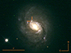 |
Fig. 1. Colour image of the host galaxy Messier 77 and of SN 2018ivc taken on 2018 November 27, four days after the explosion, with the PROMPT6 telescope. The image is a combination of the frames obtained with the B, V and R filters using the RGB technique. The SN location is marked. |
NGC 1068 (or Messier 77), is a spiral galaxy of type (R)SA(rs)b according to de Vaucouleurs et al. (1991). The galaxy hosts a well known active galactic nucleus, classified also as a Seyfert 2 galaxy (Osterbrock & Martel 1993). The Milky Way reddening in the direction of NGC 1068 is AV, MW = 0.091 mag (Schlafly & Finkbeiner 2011); however, the internal reddening is much larger and uncertain, as discussed in Sect. 4.4.
The NASA/IPAC Extragalactic Database (NED1) reports 11 measurements of distance to NGC 1068. We adopt the most recent estimation, which corresponds to a distance modulus (μ) of 30.02 ± 0.39 mag (Nasonova et al. 2011) obtained through the Tully-Fisher method. This translates into a distance of 10.1 Mpc, which is the same distance assumed by B20. The redshift of NGC 1068 z = 0.003793 ± 0.000010 (Huchra et al. 1999) corresponds to an heliocentric radial velocity of 1137 ± 3 km s−1.
3. Photometry
3.1. Observational facilities
The photometric follow-up of SN 2018ivc was performed with a plethora of instruments and telescopes around the world, made available to our collaborations. Their characteristics are reported in Table 1. Observations were made in the optical with Open, Johnson-Cousins (JC) BVRI, Sloan ugriz, and ATLAS cyan, orange (c, o) filters, and in the near-infrared (NIR) with JHKs filters.
Observational facilities and instrumentation used in the photometric follow-up of SN 2018ivc.
3.2. Data reduction
For the photometric data reduction, we used a dedicated pipeline called SNOoPY2. The instrumental magnitudes were determined through the PSF-fit method. For Sloan filter images, the photometric zero points and colour terms were computed through a sequence of reference stars from the Sloan Digital Sky Survey (SDSS) survey in the SN field. For JC BV filters, the magnitudes of the reference stars were taken from the AAVSO Photometric All-Sky Survey DR10 catalogue3. To calibrate the frames in JC RI, we converted the gri magnitudes of the SDSS standard stars in the field into BVRI magnitudes, adopting the conversion formulas of Smith et al. (2002) (see their Table 7). Finally, for NIR images, the magnitudes were calibrated with the 2MASS catalogue (Skrutskie et al. 2006). Photometric errors were estimated through artificial star experiments, also accounting for uncertainties in the PSF-fitting procedure.
Because of the complex environment around the SN, we used the template-subtraction technique4 to remove the background underlying the object. For the JC I and Sloan filters, the archive images of the SDSS DR125 survey were used as templates, while for BVR filters we chose the FORS2 images taken at the European Southern Observatory (ESO) Very Large Telescope (VLT) on 13 September 2016. Open filter magnitudes were calibrated as SDSS Sloan-r ones, because the quantum efficiency of the detector peaks at a wavelength near the maximum sensitivity of that filter.
We caution that we found a discrepancy between our Sloan g-band photometric measurements and those published by B20; these details are discussed in Appendix A.
3.3. Light curve evolution
Because of the treatment of the Open filter images as Sloan-r, the light curve in this filter is optimally sampled, especially in the earliest phases. It is used as a reference to describe the evolution of the light curves of SN 2018ivc.
The CHASE survey, using the PROMPT1 telescope, reports an upper limit on 22 November 2018. The non-detection is not stringent, at only 18.3 mag. At the beginning of the following Chilean night (November 23.03), we registered the last non-detection, this time a much deeper one (> 19.7 mag, with a threshold at 2.5σ). However, 2.5 hours later (Nov 23.13), we observed the first detection of a new source at mag 18.9 ± 0.2. Another 2.5 hours later (Nov 23.24), the transient had reached mag 16.9 ± 0.05. Consequently, in about five hours, SN 2018ivc increased in brightness by at least 2.8 magnitudes, which is equivalent to > 13.3 mag day−1. However, between the first and second detection (second and third PROMPT observations) the rise was even faster, with an increase of 2 mag in just 2.5 hours, or a rate of 18.2 ± 2.1 mag day−1. The Japanese amateur astronomer K. Itagaki detected the object eight hours after our third image (Nov 23.59) at mag 15.46. Thus, SN 2018ivc rose by more than four magnitudes in less than 14 hours. We performed a parabolic fit (i.e. a ‘fireball model’) of the fluxes of the first three detections of November 23 (the first two from CHASE plus the Itagaki’s measurement, Fig. 2) to better constrain the explosion epoch as the instant the flux is equal to 0. Interestingly, the zero flux is found at MJD 58445.108, only half an hour before the first PROMPT detection, consistent with our assumed interval for the explosion epoch (see below).
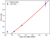 |
Fig. 2. Parabolic fit on the fluxes of the three detections of November 23. The explosion is predicted to occur when the curve crosses the zero flux level, at MJD 58445.11. The last upper limit is shown as a downwards triangle. |
While our last non-detection is not much fainter than the first detection, it is nonetheless the most stringent upper limit available from TNS or from the literature. We cannot exclude a scenario with a slower rise just after the explosion and before our observations. Finally, we also made use of our hydrodynamical modelling of the light curve, presented in Sect. 5.3, to provide an independent constrain of the explosion epoch, as described in the Appendix B. For all of the above reasons, we assume the explosion epoch as the middle point between the last upper limit and the first detection, on MJD 58445.08 (Nov 23.08). In Fig. 3 we show four cut-outs of the template-subtracted images from the PROMPT telescopes on the night of November 23, and at maximum light the night after, showing how the object has increased in brightness in just five hours and in the first 24 hours.
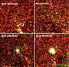 |
Fig. 3. Four stamps of the template-subtracted images from the PROMPT telescopes of 23 November 2018, showing the fast rise of SN 2018ivc after the explosion. Top-left: last non-detection with a threshold of 2.5σ. Top-right: First detection. Bottom-left: second, much brighter detection of the night. Bottom-right: First PROMPT image from the following night, with the source close to maximum light. The colour scales are roughly the same on all the stamps. All the green circles are centred on the position of the transient calculated by the PSF fitting and have a radius of 5″. |
The next day, the DLT40 survey officially discovered the transient. At that epoch, the object was already near maximum light, at Clear mag 14.65. We then initiated the multi-band follow-up campaign. The complete photometric evolution of SN 2018ivc over one year of follow-up is plotted in Fig. 4, left panel.
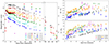 |
Fig. 4. Open, JC BVRI, Sloan ugriz, ATLAS c, o and NIR JHK light curves (left) over the one-year follow-up of SN 2018ivc. The graph has been broken into two windows (before and after +3 months) for clarity. Downward triangles mark upper limits. B − V and V − R reddening-corrected colour curves (right) of SN 2018ivc (filled points) and of the comparison objects: SNe 1993J, 2001fa, 2007fz, 1996al, and 1998S. For SN 2018ivc, we considered both the low (orange circles) and high (blue diamonds) reddening scenarios (see Sect. 4.4). |
The Open+r-band light curve can be divided into four distinct phases: a very fast rise to maximum light, reached just 1.5 days after the first detection, a first, steep linear decline, a short-duration plateau and a long, shallower linear decline. The timescale to maximum light described above is considerably short with respect to the median value of a large sample of SNe II (7.5 ± 0.3 days; González-Gaitán et al. 2015), though it has been observed in at least one other object (the sub-luminous type IIP SN 2005cs, Tsvetkov et al. 2006; Pastorello et al. 2009). After the maximum, SN 2018ivc started to fade linearly, with a slope of 13.5 ± 0.3 mag (100 d)−1. This fast linear decline only lasts 4.5 days and is followed by a short-duration phase at nearly constant luminosity, resembling a plateau lasting for about 10 days. In the redder bands a short plateau is observed, in the V and g filters the light curves show a change in the slope, becoming almost flat, while in the B filter the flattening feature is absent. Later on, the object started again to fade with a second linear decline of 3.7 ± 0.2 mag (100 d)−1, which is observed up to 3 months after the explosion, when the object went behind the Sun. However, this decline seems not to be monotonic, for example, at around +30 days it slightly slows down in the r-band. B20 also noted the short plateau and the second flattening in their light curve at the same phases and interpreted those as a signature of interaction between the SN ejecta and the CSM around the progenitor. A 2 week plateau, between +5 and +18 days, is observed in the i- and z-band light curves. Unfortunately, the NIR campaign started too late to verify whether this short plateau was also visible in the JHK filters.
Observations conducted between August and October 2019, after the Solar conjunction, show that a linear decline still ongoing, but at a shallower rate: in the V-band the rate of decline between +250 and +380 days is 1.2 ± 0.1 mag (100 d)−1, similar to other SNe II (see the s3 parameter values in Anderson et al. 2014b). In contrast, the r- and i-band light curves around +300 days are more flat, probably due to an intensification of the Hα and Ca II NIR emission lines, respectively; this is likely caused by stronger interaction. The object was still detected in Hubble Space Telescope (HST) images taken on 2 December 2020 (+740 d), at F555W = 22.71 ± 0.02 and F555W = 21.97 ± 0.03 Vegamag (Baer-Way et al. 2024).
In September 2022, one month after the ALMA observations of Maeda et al. (2023b), where they observed a radio rebrightening of SN 2018ivc, we imaged the field of the object with the 8.2-m VLT+FORS2, under favourable sky conditions (seeing ∼0.7–0.8″), in the r-band. Remarkably, we detect a source at the SN position at r = 21.1 mag four years after the explosion. SN 2001ig is another SN IIb that showed modulations and bumps in its radio light curve (Ryder et al. 2004) and was detected in the optical three years after the explosion (Ryder et al. 2006). In that case, the radio re-brightenings were interpreted as due to interaction with CSM shells produced in a binary system, with the optical detection being the survived massive companion star.
3.4. Colour curves
Based on the peculiarity of the early light curve, with a linear decline but with a short-duration plateau, and the strong He I lines in the spectra (see Sect. 4), we constructed a small sample of comparison objects. We selected the transitional type IIL SNe 2001fa and 2007fz (Faran et al. 2014), the type IIb SNe 1993J (e.g. Matheson et al. 2000a,b), 2011fu (Morales-Garoffolo et al. 2015), and 2013df (Morales-Garoffolo et al. 2014), and the type IIn SNe 1996al (Benetti et al. 2016) and 1998S7 (Leonard et al. 2000; Fassia et al. 2001; Pozzo et al. 2004).
We calculated the extinction-corrected B − V and V − R colour curves of SN 2018ivc, assuming both host reddening scenarios (discussed in Sect. 4.4) and compared them with the comparison objects. The colour curves are plotted in Fig. 4, right panel. Both the B − V and V − R colours become rapidly redder from the first observation up to ∼1 month after the explosion. Then, the increase is slower and from +50 days onwards, the B − V colour becomes bluer again.
In the low internal reddening scenario, the colours of SN 2018ivc are more similar to those of SNe 1993J and 2007fz, while in the high reddening scenario they are more akin to SN 2001fa and the SNe IIn 1996al and 1998S (the latter always remains much bluer, but the (B − V)0 colours are the same between +30 and +40 days). Type IIn SNe are known to show bluer colours due to the contribution of the ejecta-CSM interaction, which makes the continuum bluer with respect to other sub-types of SNe II (Hillier & Dessart 2019; Rodríguez et al. 2020).
3.5. Absolute light curve and rise slope comparison
We constructed the absolute r-band light curve of SN 2018ivc, with the adopted μ and the low host reddening case of AV, host = 1.5 ± 0.2 mag, as discussed in Sect. 4.4. Given the very fast rise the first day after the explosion (with a rate of 18 mag in 1 day), we chose to compare it with the rise of objects for which there is a claim of SBO detection; namely, the type IIb SN 2016gkg (Bersten et al. 2018) and the two type IIPs KSN 2011a and KSN 2011d (Garnavich et al. 2016, but see Rubin & Gal-Yam 2017). We note that the latter two were discovered by the Kepler spacecraft. The prototypical type IIb SN 1993J (Wheeler et al. 1993; Richmond et al. 1994; Woosley et al. 1994) was also used as a reference. The comparison of the absolute light curves of these four objects is shown in Fig. 5.
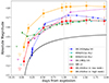 |
Fig. 5. Comparison of the absolute light curves of SNe 2018ivc, 1993J, 2016gkg (adopting the explosion epoch from Arcavi et al. 2017), KSN2011a, and KSN2011d in the first two days after the explosion. For SN 2018ivc, the Clear (calibrated as r-band) magnitudes are plotted, for SNe 1993J and 2016gkg the V-band and for the two Kepler’s SNe the KP-filter ones. For SN 2018ivc, the error bars are also plotted, summing in quadrature the errors from the photometric measurements, the μ and the internal reddening. Both the low and high host reddening scenarios are considered. The official discovery date of SN 2018ivc is marked with a vertical line. The downward triangles mark the last non-detection of each SN. The absolute r-band light curve following the SBO from a typical Wolf-Rayet model (M = 5 M⊙, R = 10 R⊙, Eexpl = 1 foe) of Nakar & Sari (2010) is also plotted (black line). |
SN 2016gkg was serendipitously observed to double in flux in just 20 minutes, which is equivalent to a rising slope of 43 ± 6 mag d−1 (Bersten et al. 2018); the fastest SN rise known to date. The hydrodynamic simulation of Bersten et al. (2018) reveals that this behaviour is consistent with the rise during the SBO phase. Compared with the rise we observed in SN 2018ivc (18 ± 2 mag d−1), the rise of SN 2016gkg is much faster. However, because the SBO rise and cooling has a typical duration of much less than 2.5 hours (see the hydrodynamic models from Bersten et al. 2018 and Tominaga et al. 2011), it could also have occurred in SN 2018ivc between the first and second CHASE observation. In this case, SN 2018ivc could have risen even faster than observed, and a higher temporal cadence of the survey may have spotted the SBO signature. Another possibility is that the CSM might have created an extended pseudo-photosphere, which would cause the SBO to last for days; hence, making it blend with the rising light curve. However, another possibility is that we actually missed the SBO because it occurred before our first observation. In fact, our last pre-discovery upper limit is not stringent enough to rule out an explosion epoch earlier than the one we assumed.
The Kepler mission claimed to have observed the SBO rise of two type IIP SNe, thanks to the fast cadence of its instrument. KSN 2011a rises faster than the model prediction by Rabinak & Waxman (2011); this was interpreted as being due to the SN shock propagating into the CSM, which allowed for the conversion of more kinetic energy into luminosity and dilute the SBO signal (Ofek et al. 2010; Chevalier & Irwin 2011; Garnavich et al. 2016). Between the first two detections, KSN 2011a has a rise slope of 5.9 mag d−1; taking into account the last non-detection, a lower limit for the rise slope of 11.5 mag d−1 was obtained. This is still slower than that observed in SN 2018ivc. In KSN 2011d, the cooling after the SBO was indeed observed (i.e. the light curve was declining just after discovery), but the rise was not. From the last non-detection, we can derive a lower limit of the slope of the rising as 11.3 mag d−1. The selected objects show heterogeneous behaviours (especially before 0.5 d), which are probably due to the different physical conditions of the exploding stars and their close environments.
4. Spectroscopy
Together with the photometric follow-up campaign of SN 2018ivc, we started a spectroscopic one, that lasted two months and during which we collected nine optical spectra, whose log is reported in Table 2. The classification spectrum is the one obtained at the Asiago Observatory, even if an earlier spectrum from the Kanata Observatory is available8.
Log of the spectroscopic observations of SN 2018ivc.
4.1. Data reduction
The spectra were pre-reduced and calibrated using standard IRAF routines, including correction for bias and flat-field, extraction of the 1D spectrum, removal of background and cosmic rays, and wavelength and flux calibrations, using arc lamps and spectrophotometric standard stars. The spectra were also corrected for the strongest telluric absorption bands. The spectra from the NOT telescope were reduced using the ALFOSCGUI9 pipeline, designed specifically for the quick reduction of photometric and spectroscopic data taken with the ALFOSC instrument, in the frame of the NOT Unbiased Transients Survey (NUTS) project (Mattila et al. 2016). The spectra from the NTT telescope were collected through the extended European Southern Observatory Spectroscopic Survey of Transient Objects (ePESSTO; Smartt et al. 2015) collaboration, and reduced with a pyraf-based pipeline (PESSTO), optimised for the EFOSC2 instrument.
The subtraction of the underlying background was particularly difficult because the object is located at the edge of the brightest part of the galaxy disk (as can be seen in Fig. 1). Hence, the contamination from the host, in the form of forbidden and narrow Balmer emission lines, is strong and spatially variable in the neighbourhood of the SN (they are stronger towards the centre of the galaxy and fainter outwards).
Finally, the spectra are corrected for the redshift of the host galaxy and the Galactic reddening, but not for the internal one, because of its uncertainties (Sect. 4.4). The sequence of spectra is shown in Fig. 6.
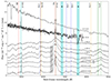 |
Fig. 6. Spectral sequence of SN 2018ivc, spanning two months of evolution after the discovery. The phases relative to the explosion are reported. The spectra have been corrected for redshift and Milky Way extinction only, as the host galaxy reddening is highly uncertain. The principal identified transitions are highlighted with vertical dashed lines. The possible high velocity feature discussed in Sect. 5.2 is also marked in gray. Each spectrum is shifted by a constant for graphical purposes. The regions most affected by the telluric absorption bands are marked in cyan. |
4.2. Line identification and spectral evolution
In the earliest spectra, over a blue featureless continuum, narrow emissions from the host galaxy are detected: those are narrow Hα and Hβ, [O III] λλ4959,5007, and [N II] λ6584. This latter line is present in all the spectra, and its contamination deteriorates the profile of the Hα line from the SN. An absorption line from the unresolved Na ID doublet is already visible, suggesting the presence of a conspicuous internal extinction along the line of sight. We also tentatively identify another absorption from the Na I λ8195.
Starting from the +10 days spectrum, a broad emission from the Ca II NIR triplet appears, each line (after a deblending) with a vFWHM between ∼6500 and ∼8000 km s−1, and it increases in strength over time. Hα now presents a broad component, with a FHWM of 12 000 km s−1, from the fast SN expanding ejecta. To the blue side of Hα, a broad bump (with a FWHM close to the one of Hα line) from He I λ5876 is visible, apparently with a broad P Cygni profile, and the strong absorption from Na I on top of the line. The blue part of the spectrum is characterised by some emission features from broad Hβ and blends of metal lines, likely due to Fe II. The principal features are located at 5000–5500 Å and 4400–4700 Å. Later on, as the continuum fades, these features become more prominent.
In the following ten days, the velocities derived from the width of the lines slightly decrease, with the FWHM of the now boxy shaped Hα going down to ∼11 000 km s−1, while the FWHM of He I λ5876 and Hβ diminish to 7000 and 8000 km s−1, respectively. The broad absorption of He I λ5876 to its blue side is also somewhat boxy in shape.
We collected three spectra at later phases (between +46 and +58 d) that are quite similar to each other. The expansion velocity from the width of the Hα line has diminished to about 8000 km s−1. Overall, the velocity evolution of H features is consistent with that found by B20, where spectra at similar phases are available. The velocity evolution of the Hα line in SN 2018ivc is shown in Fig. 7, where is compared to the sample of SNe IIP/IIL from Gutiérrez et al. (2017) and to some notable SNe IIb.
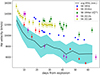 |
Fig. 7. Comparison of velocities from Hα in spectra of SNe 1993J, 1996al (considering the blue component of Hα), 2011fu (Kumar et al. 2013), 2011dh (Marion et al. 2014) 2018ivc (this work), and a sample of SNe IIP/IIL (Gutiérrez et al. 2017, using the minimum of the Hα absorption). For SN 2018ivc, the velocity is derived from the position of the minimum of the absorption. |
In the red part of the late spectra, two other emission lines from He I are detected, namely the λ7065 and λ7281, with a vFWHM ∼ 4000 km s−1. The detection of strong He I lines is typical of type IIb SNe, but in those objects the Balmer lines fade away at late phases, while in the spectra of SN 2018ivc Hα is always the strongest line. However, the spectroscopic follow-up campaign did not last sufficiently long to check if the Balmer lines disappeared in the months after the explosion. Because the three late spectra were taken closely in time, and appear very similar, we average-combined them in a single, higher signal-to-noise spectrum, that is used for the comparisons in Sect. 5.
In the +49 d Keck-I/LRIS spectrum of SN 2018ivc published by B20, a narrow Hα emission line with a P Cygni profile is visible on top of the broad Hα emission (Fig. 8). This line seems to be present also in their FLOYDS +48 d spectrum, and more marginally in our +53 and +58 d spectra. Although the narrow emission can be contamination from the host galaxy, as the [N II] λ6584 line is still visible, there is the possibility of a wind or an expanding shell in front of the ejecta, producing the narrow P Cygni absorption. This would indicate the presence of a CSM with a complex structure around the progenitor (Dessart & Hillier 2022). The expansion velocity of this putative shell, derived from the position of the minimum of the P Cygni absorption, is 250 km s−1. The same CSM velocity was measured in SN 1996al (Benetti et al. 2016). According to Smith (2014), this wind velocity is definitively fast for a RSG, and compatible with a more compact progenitor, such as a blue supergiant or a He star.
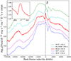 |
Fig. 8. Hα line of the +49 d Keck-I/LRIS spectrum of SN 2018ivc published by B20. The rest-frame Hα wavelength is marked and coincides with the narrow Hα emission with a narrow P Cygni profile. The HV feature at 6400 Å is visible on the left side (see Sect. 5.2). A 2m Faulkes/FLOYDS spectrum taken the day before the Keck-I one, also reported in B20, already shows the narrow absorption feature. Our lower-resolution spectra taken near that phase are also shown, in which a ‘small’ emission feature is visible at rest-frame zero velocity. A zoom on the P Cygni feature in the Keck spectrum is plotted in the blow-up box. |
B20 noted an emission feature to the blue side of Hα at ∼6400 Å, which is present also in our spectra of SN 2018ivc (see Figures 6 and 8). The feature is present in all the spectra between phase +15 and +60 days and is strongest in the +22 and +46 d spectra, when the r-band light curve presents a change in the declining slope. They interpreted it as a high velocity (HV) blue-shifted emission feature from the Hα line, generated in a fast-moving (∼104 km s−1) clump, approaching the observer. The identification of this feature as [O I] λλ6300,6364 is not ruled out; however the rest-frame central wavelength of this feature changes from 6360 to 6415 Å between phase +15 d and +46 d. If this feature would be from the [O I] λ6300 transition, it would be redshifted by a velocity increasing with time from +2850 km s−1 to +5400 km s−1. Therefore, it is easier to explain this feature as a slowing-down Hα HV feature instead. Also, our spectra were taken too early for the SN to have entered in the nebular phase, when [O I] lines are typically observed.
Looking again at Fig. 8, we note the emergence of a broad shoulder to the red at ∼+4000 km s−1 over time, while the peak of the broad Hα is offset by about −2000 km s−1 to the blue (see also Anderson et al. 2014a). This, together with the presence of the HV feature, suggests that the ejecta are strongly asymmetric.
4.3. Comparison with various objects
We used the tool GELATO (Harutyunyan et al. 2008) to search for objects with spectra similar to those of SN 2018ivc, both at the early and late phases. Interestingly, at +1.5/+2 d the software finds a match with two well-known type IIn SNe, 1996al and 1998S. B20 interpreted the deviations from the linear decline in the light curve as evidence of interaction between the fast SN ejecta and a CSM, which would make SN 2018ivc an interacting SN. However, the spectra of SN 2018ivc never show narrow H emission lines, usual indication of the presence of a CSM surrounding the progenitor star. Therefore, SN 2018ivc cannot be considered as a type IIn SN. Running on the early spectra, GELATO gives two type IIb events, SNe 1993J and 2011fu as comparison objects. This is in agreement with the presence of intense He I emission lines. The early spectrum of SN 2018ivc and the spectra of the comparison objects are plotted in Fig. 9.
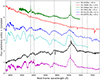 |
Fig. 9. Comparison of an early spectrum of SN 2018ivc (+10 d) with those at similar epochs of SNe IIn 1996al and 1998S, SNe IIb 1993J and 2011fu, SN IIL 2007fz. The true spectral appearance of SN 2018ivc in the first days is hidden by the effects of interaction. H and He transitions are marked by the continuous and dashed vertical lines, respectively. |
4.4. Internal extinction
The deep absorption from the Na I D λλ5890,5896 doublet indicates the presence of a non-negligible internal extinction. We measured the equivalent width (EW) of the unresolved doublet in all the available spectra, and calculated a mean value of 3.0 ± 0.4 Å. This value is not useful for accurately estimating the dust extinction, as the relations by Poznanski et al. (2012) and Munari & Zwitter (1997) between the EW of the Na I doublet and the extinction from the host galaxy saturate for EW > 0.8 and > 0.6 Å, respectively. The saturation of the Na I lines precludes a precise measure of AV,host, but it is likely high. The relation by Turatto et al. (2003), despite being likely saturated, would provide an additional reddening from the host of AV,host = 1.5 ± 0.2 mag. Finally, we use the relation of Rodríguez et al. (2023) valid for SNe II to estimate a lower limit on the host galaxy extinction of AV,host ≥ 1.4 ± 0.3 mag. These values are similar to that assumed by B20 who, from a HST pre-explosion image of the field of SN 2018ivc, and from measurement of the Balmer decrement in a VLT+MUSE spectrum of the SN site years before the explosion, estimated a colour excess E(B − V)≈0.5 mag.
As the type IIn SN 1996al is a comparison object to SN 2018ivc, given its similar light curve evolution and early spectra, we tried to correct the B − V colour curve of SN 2018ivc to match that of SN 1996al at early phases. We interpolated the (B − V)0 colour curve of SN 1996al between the discovery and +50 d phase and calculated the median difference of B − V colour between the two objects, to get the same average colour evolution. We found a colour excess of E(B − V) = 1.04 ± 0.04 mag (AV = 3.22 ± 0.09 mag, of which 0.09 mag from the MW). By matching in the same manner the V − R colours between +20 and +70 d we derived a total colour excess E(V − R) = 0.63 ± 0.04 mag (equivalent to E(B − V) = 1.21 ± 0.08 mag).
From our long-slit spectroscopy of SN 2018ivc, we extracted the spectra of three different H II regions adjacent or close to the SN position, that fell within the slit when our spectra were taken. The H II regions selected are highlighted in Fig. 10. In particular, we measured the flux of Hα and Hβ emission lines to evaluate the Balmer decrement. From three different spectra, we obtained an average Hα/Hβ ratio of 7.5 ± 0.5. Using the relation by Botticella et al. (2012) (their Equation 8), and AV/AHα = 1.22 (Cardelli et al. 1989), we derived an additional host extinction of AV, host = 3.0 ± 0.2 mag, which assuming RV = 3.1 gives E(B − V)∼1.0, double what we obtained from the Na I D EW and the value assumed by B20. The internal extinction we derived from the Balmer decrement of nearby H II regions close to the SN explosion site is much higher than that adopted by B20, but it is also similar to the one necessary to obtain a match between the colour curves of SN 1996al and SN 2018ivc. This makes the internal reddening very uncertain, and might be variable across the region. Therefore, we will not prefer one estimation or the other but evaluate both scenarios equally. We will consider the case of an internal extinction of AV,host = 1.5 mag (from the Na I doublet) as the ‘low reddening scenario’, while the case of AV,host = 3.2 mag (from the B − V colour comparison with SN 1996al and the Balmer decrement of close-by H II regions) as the ‘high reddening scenario’.
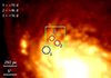 |
Fig. 10. Archival r-band image from the Dark Energy Survey DR1 of the field of SN 2018ivc. The cross marks the SN position. The field-of-view of VLT+MUSE in narrow-field mode is shown by the square. The H II regions from which we extracted the spectra to evaluate the Balmer decrement are highlighted by the circles. |
In their recent work, Maeda et al. (2023a) estimated an upper limit of ≲0.015 M⊙,on the ejected 56Ni mass of SN 2018ivc from observations with ALMA, assuming the low reddening scenario and that the 56Ni heating is not a main power source for the optical luminosity. This value is a factor of ∼4 − 5 smaller than that determined for the canonical type IIb SN 1993J (∼0.07 M⊙; Nomoto et al. 1993; Woosley et al. 1994). Instead, in the high reddening case, the upper limit would be larger, at ∼0.07 − 0.08 M⊙.
4.5. Bolometric light curve
We constructed the pseudo-bolometric light curve of SN 2018ivc from the contribution from u− to z− bands. For epochs without observations in some bands, we interpolated the available data using the r-band light curve as reference and assuming a constant colour index. For the phases between ∼35 and ∼70 days, when the NIR magnitudes are available, we calculated the pseudo-bolometric luminosity including also the contributions from JHK bands. In the high-reddening scenario, the NIR bands add a 15% contribution to the bolometric flux, while this increases to 50% in the low-reddening one. However, as the NIR measurements are too few, we did not try to extrapolate the JHK light curves with the assumption of a constant colour.
The entire pseudo-bolometric light curves (for the low and high reddening scenarios) are shown in Fig. 11, with a blow-up on the first two months in the inset inbox. In early phases, we see a steep decline, which is slightly slower between +10 and +20 days, in correspondence with the short-duration plateau observed in the redder bands. Instead, at phases later than +90 d, the rate of decline is shallower, at 0.92 ± 0.07 mag (100 d)−1, only slightly slower than the decay of 56Co (0.98 mag (100 d)−1), though within the error bar can also be compatible with it.
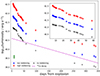 |
Fig. 11. Pseudo-bolometric uBgVrRiIz light curves of SN 2018ivc, for both the low and high reddening scenarios. The inset shows a blow-up of the first two months after the explosion. For reference, we plot also the pseudo-bolometric light curve without any correction for reddening in black; the short plateau feature is more pronounced. The decay slope of 56Co (0.98 mag (100 d)−1) is reported with a dashed purple line for comparison. At late phases (after +100 days) the evolution of SN 2018ivc is close to being powered by the 56Co decay. The systematic error bar due to the uncertainty on the distance is reported in the bottom-left corner. |
We estimated the ejected 56Ni mass of SN 2018ivc from the ratio of its bolometric luminosity at the last three epochs (+285 d, +333 d and +339 d) and that of SN 1987A at the same epochs. For SN 1987A, the pseudo-bolometric luminosity was calculated accounting for the contribution of the UBVRI bands. In the low reddening scenario, the average ratio found is Lbol(1987A)/Lbol(2018ivc ; assuming a M(56Ni) of 0.075 M⊙, for SN 1987A (Woosley et al. 1989), the 56Ni mass derived for SN 2018ivc is 1.1
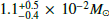 . Instead, in the high reddening case, the ratio obtained is Lbol(1987A)/Lbol(2018ivc
 , hence a mass of 56Ni for SN 2018ivc of 4.2
 . The estimated 56Ni mass, even in the high reddening case, is in the lower part of the M(56Ni) distribution of SNe IIb: from the analysis of 45 objects of this type, Rodríguez et al. (2023) found that the average 56Ni mass produced by SNe IIb is 0.066 ± 0.006 M⊙. The M(56Ni) of SN 2018ivc, low for a SN IIb (see also Morales-Garoffolo et al. 2014; Gangopadhyay et al. 2018 and the samples of Anderson 2019; Meza & Anderson 2020; Afsariardchi et al. 2021), may explain the missing second 56Ni-heating powered peak in the light curves, substituted instead by an interaction-powered plateau (Maeda et al. 2023a). We remark that the above estimates of the M(56Ni) are likely only upper limits due to the powering contribution of the interaction to the light curve, even at late phases, as demonstrated by our modelling (see Sect. 5.3) and by the late-time rate of decline of the bolometric light curve, which is shallower than that expected from 56Co decay.
5. Discussion
5.1. A transitional SN IIL/IIb?
Light curves of SNe IIb are typically characterised by a first luminous peak a few days after the explosion, a local minimum and then a second maximum about three weeks later. In some objects (SNe 1993J and 2011fu, more evident in the bluer filters) this second peak is fainter than the first one.
Between phases +5 and +20 d, the light curves of SN 2018ivc in the red filters show a plateau, while in a few type IIb SNe (1993J, 2011fu and 2013df; figure 4 of Morales-Garoffolo et al. 2015) a secondary maximum is observed at about the same phase. The absence of a local minimum in the light curve of SN 2018ivc, at the time when the short-duration plateau is visible instead, might be explained by the additional radiation from the interaction between the fast ejecta and a CSM. This is supported by the similar photometric behaviour presented by the SN IIn 1996al, even though narrow emission lines are not present in SN 2018ivc, and by the results of our hydrodynamical modelling (see Sect. 5.3).
SNe 2007fz and 2001fa (Faran et al. 2014) are two spectroscopically confirmed type IIL SNe that show a mild increase in brightness between one and two weeks after maximum, similar to that observed in some type IIb SNe. In Fig. 12, we present a comparison of the BVRI absolute light curves of SN 2007fz (together with SNe 1993J and 2001fa) to those of SN 2018ivc in the first 60 days after maximum. We note a good similarity between the two light curves, concerning both the secondary peak and the decline slope at later phases.
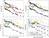 |
Fig. 12. Comparison between the BVRI absolute light curves of SNe 1993J, 2011fu and 2013df (IIb), 1996al (IIn), 2001fa and 2007fz (IIL), and 2018ivc up to 60 days after maximum. For SN 2018ivc, the absolute light curves for both the low and high reddening scenarios are plotted with circles and squares, respectively. SN 2007fz presents a well-defined secondary peak between one and two weeks after maximum, while SN 2018ivc shows a short plateau. The two objects have quite similar photometric evolution. |
The second, long linear decline and the late spectrum appearance would make SN 2018ivc a type IIL SN; however, the presence of He lines and some resemblance of the early spectra with those of SNe 1993J and 2011fu are more coherent with a type IIb classification. As a comparison, in the three late time spectra of SN 2018ivc, we measure a mean intensity ratio Hα/He I λ5876 ≃ 8.4 ± 0.7. In the spectra of type IIL SNe from the sample of Faran et al. (2014), at phases in the range of +23 to +90 d, the measured ratios are distributed between 4 and 21, but with a majority around 7 (see Fig. 13). Differently, in the spectra of SNe IIb 1993J (from Barbon et al. 1995), 2011fu and 2013df between +42 and +62 days, the measured ratios are between 2 and 3, clearly separated from the distribution of values for SNe IIL. According to these measurements, SN 2018ivc belongs to the family of SNe IIL rather than SNe IIb, though it has to be noted that interaction may change the ratio.
 |
Fig. 13. Histogram of the distribution of the average flux ratio Hα/He I λ5876 in three SNe IIb (SNe 1993J, 2011fu and 2013df, in blue), nine SNe IIL from Faran et al. (2014) (in red) and SN 2018ivc (in green) between one and three months after the explosion. The majority of SNe IIL have a Hα/He I λ5876 ratio of around 7, with some outliers, while SNe IIb have a ratio between 2 and 3. With a ratio of 8.4, SN 2018ivc would be a type IIL SN. |
Finally, in Fig. 14 we compare the late average spectrum of SN 2018ivc with those of a sub-sample of both type IIL and type IIb SNe, to see which category the object studied in this work may belong to. SNe IIL are characterised by a strong Hα, with faint or absent He I emission lines. On the contrary, SNe IIb show prominent lines from He I, while Hα is not visible. By this spectroscopic comparison, SN 2018ivc seems more related to SNe IIL, but with a peculiar light curve. In this sense, probably the best comparison object to SN 2018ivc is SN 2007fz: they have similar Hα profiles, He I lines, Ca II NIR triplet and the blue bump at 4600-4700 Å. Instead, SN 2001fa has a spectrum closer to that of a normal type II SN, lacking the He I emission lines.
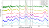 |
Fig. 14. Comparison of the late mean spectrum of SN 2018ivc (+52 d) with those of some reference types IIL and IIb SNe, taken at late phases. The sample includes: SNe 1993J, 2011fu and 2013df (Shivvers et al. 2019) for type IIb, SNe 2001fa and 2007fz (Faran et al. 2014) for type IIL. SNe IIL have strong Hα and faint or no He I lines, the opposite is true for SNe IIb. Hα and the principal He I lines are marked by the vertical continuous and dashed lines, respectively. |
Nonetheless, in their recent paper, Maeda et al. (2023a) suggested the SN type of SN 2018ivc as IIb, based on various indications. The argument was further confirmed by Maeda et al. (2023b) thanks to late-time ALMA observations at 100 and 250 GHz frequencies, which revealed rebrightening synchrotron emission that is consistent with the history of prolonged mass ejection episodes before the explosion proposed by their SN IIb-IIL transition interpretation.
5.2. A possible interacting SN IIL
The light curve of SN 2018ivc, during the early phases of evolution, presents some flattenings (or changes in the declining slope), which are typically interpreted as an indication of an on-going interaction between the SN ejecta and a pre-existing CSM. This interaction is generally revealed by the presence in the spectra of narrow emission lines, from the Balmer series, on top of a much broader component, produced in the fast-moving ejecta.
However, while we detected variations in the slope of the light curve during the post-maximum declining phase, the spectra never show narrow emissions lines. In Fig. 9, we compare the early spectra of SN 2018ivc to those of different SN subtypes, specifically SNe IIn, from which it is clear that SN 2018ivc does not show the typical features of interacting SNe.
We see the velocity of the HV feature described in Sect. 4.2 to slow down with time, as already noted by B20. The highest velocity, derived by measuring the position of its peak in the +16 d spectrum, is −9500 km s−1, while the lowest is measured in the +53 d spectrum, at just −7000 km s−1. in Fig. 15 we plot a zoom on the Hα HV feature in the velocity space, where it is evident the movement with the phase towards the red, indicating its slowing down. The feature seems to be present also in our +46 d spectrum at ∼8330 Å. If it is associated to the Ca II λ8542 transition, its recessional velocity would be −7400 km s−1, consistent with that of the Hα HV feature in the same spectrum. A HV feature may indicate the presence of an asymmetric structure, with which the SN ejecta later interacted. The CSM may have had a bipolar shape, while the ejecta are more spherically symmetric, or vice-versa. Two HV features (one approaching and one receding) were observed in the Hα profile in the spectra of type IIn SNe 2010jp (Smith et al. 2012) and 2014G (Terreran et al. 2016), and they offered this interpretation to explain them. When the fast ejecta interact with a slow-moving CSM, part of its kinetic energy is converted into radiation. This can explain why the velocity slows down from the spectral features of SN 2018ivc at around +1 month, also compared to the average velocity of SNe IIP/IIL (Gutiérrez et al. 2017).
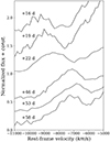 |
Fig. 15. Zoom on the HV feature on the blue side of Hα in the rest-frame velocity. The velocity of the feature clearly slows down with the phase. |
If indeed SN 2018ivc is also a transitional object between normal type II and interacting SNe, it could point in favour of a continuous distribution in properties from SNe II towards SNe IIn, as observed in the luminous low-expansion velocities (LLEV) objects reported by Rodríguez et al. (2020). LLEV SNe show signs of ejecta-CSM interaction in their light curves during the initial months (4–11 weeks). After that, their spectra evolve as normal type II SNe. It is worth noting that LLEV SNe are much more luminous than SN 2018ivc at the characteristic phase of 50 days (∼2 mags even in the high reddening scenario), indicating a stronger interaction, which is also supported by their early appearance as SNe IIn. If this interpretation holds, the different spectral evolution is mainly related to the density profile of the CSM around the progenitor star, which reflects its mass-loss history.
On frequent occasions (see, for example, Ofek et al. 2014; Strotjohann et al. 2021; Reguitti et al. 2024), luminous outbursts during a long-lasting eruptive phase were observed a few years before the explosion of some SNe IIn. The mass-loss rate is highly enhanced during these phenomena, leading to the formation of a massive CSM (Smith 2014). We searched for pre-explosion images in the archives of major astronomical observatories and all-sky surveys for transients, looking for pre-SN outbursts from the progenitor of SN 2018ivc in the years prior (between 2000 and 2018), but found no significant variability.
As stated in the previous Section, there is a possible similarity (found by the GELATO algorithm) between the early spectra of SN 2018ivc and those of the type IIn SN 1998S. This may support the idea of the presence of a CSM close to the progenitor star. Indeed, looking again at Fig. 14, in SN 2018ivc all the broad P Cygni features from H, He, and Ca are shallower than in the comparison objects. This could be an effect due to interaction with a CSM (Dessart & Hillier 2022). Yet, Smith et al. (2015) pointed out that, after the initial phases, SN 1998S too shared some properties of type IIL-like SNe. B20 found another type IIn event, the well-studied SN 1996al (Benetti et al. 2016), as the object with the most similar light curve to SN 2018ivc, because of a change in slope in the former object during the earliest phases (they even state that SN 1996al can be considered a IIn/IIL SN transition).
Searching in the literature for other transitional type IIL/IIn objects, we found one more event with behaviour not dissimilar to SN 2018ivc. PTF11iqb (Smith et al. 2015) is a changing-look SN: the spectra at very early phases (a few days after the explosion) show SNe IIn-like features, but then the spectra change and evolve towards a type II SN, while the light curve presents a plateau, typical of type IIP SNe. Finally, during the nebular phase, the spectrum returns to be more akin to that of a type IIn SN. PTF11iqb is less luminous than SN 1998S, and its emission lines are fainter, but overall the spectra of the two objects are similar. Smith et al. (2015) suggest that PTF11iqb can be explained as a normal core-collapse SN with a weaker CSM interaction than in SN 1998S. Finally, it has been argued that all SNe IIL experience at least moderate interaction in the initial phase (Valenti et al. 2015; Bose et al. 2015) (though they would not necessarily appear as SNe IIn, with narrow emission lines, if the CSM is not dense enough; Dessart & Hillier 2022). After the first days, the spectra evolved as normal type IIL or IIP SNe, as in the case of PTF11iqb. For instance, Morozova et al. (2017) demonstrated that signs of interaction were present in the light curves of the type IIL SNe 2013ej and 2013fs, even though the typical features of type IIn SNe are not revealed in their spectra (see also Bullivant et al. 2018).
5.3. Modelling of the early light curve
The early light curve of SN 2018ivc is suggested to be powered by the interaction between the ejecta and the surrounding CSM in both B20 and Maeda et al. (2023a). B20 derived an upper limit for the ZAMS mass of a ‘single star’ progenitor, estimated to be less than 11 M⊙, based on pre-supernova HST images captured at the SN’s location. In Maeda et al. (2023a), the optical bolometric light curve of SN 2018ivc has been simulated with the SN-CSM interaction model proposed in Maeda & Moriya (2022). To explain the unique behaviour of the light curve, characterised by a nearly flat evolution up to 17 days post-explosion followed by a transition phase between 20 and 30 days and, thereafter, a relatively steeper decline, Maeda et al. (2023a) proposed a two-component density profile for the CSM enveloping SN 2018ivc. This profile consists of a flatter density configuration (ρ ∝ r−1.6) spanning from 5 × 1014 cm (∼7200 R⊙) to 2 × 1015 cm (∼29 000 R⊙) from the progenitor to simulate the flat evolution until 17 days. A steeper density configuration (ρ ∝ r−2.5) until 1.5 × 1016 cm from the progenitor has been used to reproduce the steeper decline after 30 days. Furthermore, their analysis estimated the synthesised 56Ni mass resulting from the explosion to be below 0.015 M⊙, and their modelling approach did not consider any contribution from the radiation produced by the decay of 56Ni. We employed the Supernova Explosion Code (SNEC; Morozova et al. 2015), an open-source Lagrangian 1D radiation hydrodynamic code, to simulate the intriguing behaviour of the fast rise followed by a sustained plateau for ≲ 17 days post-explosion in the multi-band optical light curves of SN 2018ivc.
In the case of SN 2018ivc, we were able to record a clear and steep rise to maximum brightness, but this was only observed in the Clear band. The fast rise holds substantial importance, particularly given the limited availability of early-time data for events of such peculiar nature. It plays a pivotal role in effectively constraining the characteristics of both the CSM and the progenitor. Thus, our primary focus is centred on conducting multi-band light curve modelling using SNEC, with a specific emphasis placed on the Clear band. The SNEC simulation framework relies on the assumptions of diffusive radiation transport and local thermodynamic equilibrium. Regarding the progenitor model, we explore two scenarios:
-
A typical extended progenitor of type IIb SNe with an H envelope mass (MH) of 0.02 M⊙,
-
Stripped progenitor models with three different MH values: 0.38, 0.74 and 1.61 M⊙.
The best-fitting progenitor model is determined by finding the minimal χ2, computed as
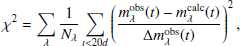 (1)
(1)
where mλobs(t) and Δmλobs(t) are the magnitudes and their corresponding errors at time t, mλcalc(t) are the computed magnitudes at time t, λ denotes the various filters, and Nλ is the total number of observed data points in filter λ. We compute mλcalc by setting RV = 3.1 and varying E(B−V) in the range of low and high reddening values.
5.3.1. Light curve modelling with SNe IIb progenitor model
In this case, the SNe IIb progenitor models are calculated by the Nomoto & Hashimoto (1988) prescription from the ZAMS to pre-explosion conditions and correspond to H-free structures. Later, an extended H envelope is attached to the He core, assuming thermal and hydrostatic equilibrium. The mixing length parameter used is 2.5, and the stellar models are calculated assuming solar metallicity (see Bersten et al. 2012). The final progenitor model used corresponds to the stellar evolution of a single star with a ZAMS mass of 15 M⊙, a radius equivalent to 350 R⊙10, a helium core mass (MHe) of 4 M⊙, and MH of 0.02 M⊙. These parameter values are typical for the extended progenitors of SNe IIb (see Chevalier & Soderberg 2010; Ouchi & Maeda 2017; Yoon et al. 2017; Sravan et al. 2019). The H-envelope mass falls in the range 0.01–0.5 M⊙ proposed by Sravan et al. (2019) for the progenitors of SNe IIb (see also Table 5 of Balakina et al. 2021), and agrees with the finding of Yoon et al. (2017) that SN IIb progenitors have a H-envelope mass ≲0.15 M⊙, but is lower than the minimum value of 0.033 M⊙ found by Gilkis & Arcavi (2022). However, according to Dessart et al. (2011), a H-envelope mass of just 0.001 M⊙ is enough to reproduce a normal SN IIb.
For the explosion, SNEC takes the progenitor and explosion parameters as input and generates a range of outputs including multi-band and bolometric light curves, and photosphere velocity evolution. However, due to the unique characteristics of SN 2018ivc, determining suitable parameter ranges for modelling posed challenges. The common two-step approach adopted in previous studies involving SNEC modelling (Morozova et al. 2018), which entails initially fitting the late-time light curve to constrain mass and explosion energy, followed by fitting the early light curve to determine CSM properties, was not as effective in this case. This is because the evolution of SN 2018ivc is suggested to be predominantly governed by the interaction between the ejected material and the CSM even during later phases (Maeda et al. 2023a).
To address this, we began by constraining the range of explosion energy through simulations of the progenitor model using SNEC. Multiple simulations were conducted with energies ranging from 0.1 to 1.0 foe (1 foe = 1051 erg), keeping the 56Ni mass fixed at 0.015 M⊙. The best fitted model from these simulations corresponds to an AV of 1.5 mag and explosion energy of 0.7 foe, capable of reproducing the observed multi-band light curves until approximately four days post-explosion. The model photospheric velocities are lower than the expansion velocities estimated from the spectra, as determined by the minima of the Fe IIλ5169 line. While increasing the explosion energy can enhance the model photospheric velocity, such models fail to reproduce the rise in the Clear band light curve. The best fitted multi-band light curve models without CSM and the photospheric velocities are depicted in Fig. 16.
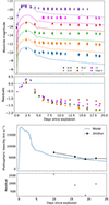 |
Fig. 16. Models evolved from the progenitor without adding CSM. The top panel displays the best fit model of the first 20 days of BVRIi and Clear light curves of SN 2018ivc. The bottom panel shows the photospheric velocity corresponding to the best fit model along with the observed photospheric velocity. |
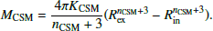
Next, we added the CSM above the progenitor models with a density profile described by the equation:
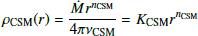 (2)
(2)
Herem Ṁ is the mass-loss rate, νCSM is the CSM velocity, KCSM is the mass-loading parameter, and nCSM is the power index of the CSM density radial distribution. Thus, Ṁ can be estimated from KCSM and νCSM.
The CSM mass can be written as
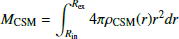 (3)
(3)
where Rin is the inner CSM radius and Rex is the outer CSM radius.
Replacing ρCSM(r) in Eq. (3) with Eq. (2) and integrating, we get
 (4)
(4)
Thus, we need to derive an expression for KCSM to estimate the CSM mass. To maintain continuity between CSM with varying densities and the progenitor, we introduced an intermediate component bounded by the progenitor radius and the inner CSM radius. While this intermediate component maintains the same density form, it utilises a distinct power value (nINT) for the radius:
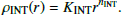 (5)
(5)
We set the density of the intermediate component at the progenitor radius equal to the progenitor density ρprog at the star’s radius (R⋆). Thus,
 (6)
(6)
Also, to maintain continuity between the intermediate shell and the CSM, the density of the CSM at Rin has to be set to the density of the intermediate shell at Rin. Thus,
 (7)
(7)
Since the density of the intermediate component at Rin can also be written as (and using KINT from Eq. (6)):
 (8)
(8)
we can finally obtain an expression for KCSM, by substituting ρINT(Rin) from Eq. (8) to Eq. (7),
 (9)
(9)
The final CSM structure is shown in Fig. 17. The kink in the density at the edge of the progenitor is required to stabilise the hydrostatic structure of the extended envelope. To accommodate CSM with different densities, we varied nINT and chose to keep the inner radius of the CSM fixed at 400 R⊙.
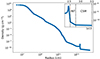 |
Fig. 17. Density profile attached to the progenitor. The inset shows a zoom-in of the intermediate component (‘INT’) attached between the progenitor and the CSM. |
Initially, we used nCSM = −1.6 in the CSM density profile, as estimated in Maeda et al. (2023a), for the inner CSM responsible for the evolution in the first 17 days. However, the inner CSM’s radius in Maeda et al. (2023a) was situated at a significantly larger distance compared to our study. Moreover, this choice resulted in a shallower rise, which did not match the steep rise observed in the Clear band light curve of SN 2018ivc. Since reproducing this steep rise was a crucial objective, we investigated how altering nCSM impacted the light curve shape. We found that increasing the value of nCSM resulted in a steeper rise in the light curve. In Fig. 18, the effect of varying nCSM on the modelled Clear band light curves up to 1.5 d post-explosion for a specific set of explosion energy, Rex, and nINT values (0.3 foe, 4000 R⊙, and −10, respectively) are shown.
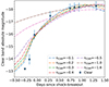 |
Fig. 18. Effect of nCSM on the rise of the Clear band light curve. Increasing the value of nCSM resulted in steeper light curves. |
The slope of the rise in the model light curves is also affected by the outer CSM radius (Rex). A higher Rex leads to a shallower rise and a broader peak. We also explored the influence of the 56Ni mass on the early light curve and found that the 56Ni mass had a negligible impact on the early light curve. Thus, we fixed the 56Ni mass at 0.015 M⊙. The 56Ni mixing parameter, which signifies the mass coordinate up to which 56Ni is distributed outward in the ejecta, was fixed at 4 M⊙. Nonetheless, this parameter had no discernible impact on the early light curve.
Considering these factors, we are left with four modelling parameters: nINT, nCSM, Rex, and explosion energy. We proceeded by generating models with explosion energies in the range 0.1–0.7 foe, incrementing in steps of 0.1 foe. For the CSM extent parameter, we systematically explored a range spanning from 1500 to 5000 R⊙, incrementing in steps of 100 R⊙. For nCSM, we explored a range from −0.5 to −0.1, with increments of 0.1. For nINT, we explored the range between −8 and −15. From these simulations, we identified the best fit parameters.
The best-fitted model correspond to Rex = 4100 R⊙, explosion energy = 0.3 foe, nCSM = −0.5, nINT = −10. The AV value for this model fit is 3.2 mag. These parameter choices yielded a model that achieved an optimal alignment with the observed multiband light curves. The best fit model and the corresponding photospheric velocity evolution are shown in Fig. 19, along with the observed multiband light curves and expansion velocities, respectively. While it is feasible to achieve a better fit for the rising portion by decreasing Rex and increasing nCSM, such an adjustment leads to a deterioration in the fit for the light curve following the initial rise. Using these parameter values in Eqs. (4) and (9), we estimate a CSM mass of 0.47 M⊙.
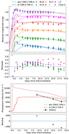 |
Fig. 19. First 20 days of the BVRIi and Clear band model light curves corresponding to the ‘stripped_6M’ model along with the observed multi-band light curves of SN 2018ivc (top). Photospheric velocity evolution corresponding to these models along with the observed photospheric velocity (bottom). |
5.3.2. Light curve modelling with stripped progenitor model
In this case, we used the stripped-mSGB series progenitor models from Morozova et al. (2015), where a ZAMS star with an initial mass of 15 M⊙ is evolved using Modules for Experiments in Stellar Astrophysics (MESA, Paxton et al. 2019; Jermyn et al. 2023, and references therein) until the middle of the sub-giant branch phase (mSGB). At this stage, a portion of the star’s mass is instantaneously removed, after which the evolution continues until the onset of core collapse. We considered progenitor models with 5, 6, and 7 M⊙ of stripping, resulting in residual MH values of 0.38, 0.74, and 1.61 M⊙, respectively. The 5 M⊙ stripped progenitor has a pre-supernova mass of 6.82 M⊙, a He core mass ofF 5.21 M⊙ and a radius of 828 R⊙. The 6 M⊙ stripped progenitor has a pre-supernova mass of 5.94 M⊙, a He core mass of 5.20 M⊙ and a radius of 663 R⊙, while for the 7 M⊙ stripped progenitor, the pre-supernova mass is 5.59 M⊙, the He core mass is 5.21 M⊙ and the progenitor radius is 555 R⊙.
To these progenitor models, we attached a wind-like density profile for the CSM (see Fig. 20) and exploded the models with SNEC. In this case, we have three free parameters: explosion energy, CSM extent (Rex) and mass-loading parameter (KCSM). We explored a range of explosion energies from 0.1 to 0.7 foe, Rex from 2000 to 4000 R⊙ in steps of 100 R⊙, and KCSM ranging from 0.5×10¹⁷ g cm−1 to 1.5×10¹⁷ g cm−1 in steps of 0.1×10¹⁷ g cm−1. The 56Ni mass and 56Ni mixing parameters are kept fixed at 0.015 M⊙ and 3 M⊙, respectively. To observe the impact of increasing the progenitor’s H envelope mass on the light curves, we depict the Clear band model light curves for the three progenitor models in Fig. 21, employing the same KCSM of 1.0×10¹⁷ g cm−1 and Rex of 3000 R⊙, which corresponds to an approximate CSM mass of 0.1 M⊙. It is evident that as the H envelope mass increases, the models better fit the light curves after 12 days. However, lower H envelope masses tend to yield higher velocities, aligning more closely with the observed velocities. Comparing the three progenitor models, the χ2 attains its minimum value for the 6 M⊙ stripped model, corresponding to a H-envelope mass of 0.74 M⊙. Nevertheless, the model velocities associated with H-envelope mass of 0.38 M⊙ better match the observed velocities.
 |
Fig. 20. Density profile attached to the stripped progenitor. The inset shows a zoom-in of the CSM profile attached. |
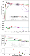 |
Fig. 21. Model light curves corresponding to the three stripped models of the first 20 days of Clear band of SN 2018ivc along with the observed Clear band light curves (top). Photospheric velocity evolution corresponding to these models along with the observed photospheric velocity (bottom). |
Finally, the best-fitted model to the multiband light curves corresponds to the 6 M⊙ stripped model with an explosion energy of 0.4 foe, Rex of 3200 R⊙ and KCSM of 0.8 × 10¹⁷ g cm−1. This would correspond to a CSM mass of 0.09 M⊙. The AV corresponding to this fit is 2.6 mag (Fig. 22).
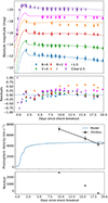 |
Fig. 22. Best fit model with the addition of CSM. The top panel features the best fit model of the first 20 days of BVRIi and Clear light curves of SN 2018ivc along with the observed multi-band light curves. The bottom panel shows the photospheric velocity evolution corresponding to the best fit model along with the observed photospheric velocity. |
An H-envelope mass of 0.74 M⊙, falls in between the values estimated for the typical progenitors of SNe IIb (up to 0.5 M⊙, Sravan et al. 2019) and SNe IIL (∼1 M⊙, for Swartz et al. 1991; 1–2 M⊙, for Blinnikov & Bartunov 1993). This is consistent with SN 2018ivc being a transitional IIL/IIb object, as confirmed by our other indicators. While an MH of 0.38 M⊙, is within the proposed range of SNe IIb progenitors, it still remains in the upper side of the range. Considering the large progenitor radius of 350 R⊙, we adopted for the SN IIb progenitor model, and 663 R⊙, for the ‘stripped_6M model’ (see Table 3), a higher MH is also consistent with the fact that more extended SNe IIb progenitors should be also more H-rich (Prentice & Mazzali 2017).
Pre-supernova structure summary and CSM parameters.
The pre-supernova configuration and the optimal CSM parameters, along with the corresponding χ2 values for the two progenitor scenarios, are summarised in Table 3. The stripped progenitor model yields the minimum χ2, corresponding to an MH of 0.74 M⊙, which is intermediate to those of IIb and IIL progenitors. Additionally, the model photospheric velocities corresponding to the stripped progenitor model are a closer match to the observed velocities than those of the type IIb progenitor model. We note that in Maeda et al. (2023a), a low-density CSM located at a greater radial distance has been favoured. Hence, the CSM we are examining here differs from the component proposed by Maeda et al. (2023a). However, a dense CSM (as used in our models) in close proximity to the progenitor would decelerate the shock, delaying the peak in radio emission, which contradicts observed radio data. Introducing such low densities near the progenitor in SNEC modelling produces light curves resembling those of ‘no-CSM’ models, capable of replicating the early rise in the Clear band, seemingly unaffected by the low-density CSM. While Maeda et al. (2023a) suggested that their CSM would negligibly affect the rising part of the light curve, placing the low-density CSM at a higher radius, as suggested by Maeda et al. (2023a), results in model light curves that appear nonphysical. Indeed, all SNEC modelling based studies have demonstrated the necessity of a confined CSM to accurately replicate observed light curves. The disparity may be reconciled with a non-spherical CSM featuring both low and high dense regions.
Additionally, the dense CSM close to the progenitor could explain the absence of narrow emission lines in SN 2018ivc, typically observed in the spectra of type IIn SNe. The dense CSM would result in a high electron scattering optical depth (≫100). Hence, the mean free path of recombination photons responsible for the formation of the narrow features will be much smaller than RCSM. The narrow features can only form in case of radiation leakage from the shock into the CSM above, and this cannot occur when the CSM density is high (on the order of 10−10 − 10−9 g cm−3, Dessart et al. 2017). For instance, at 4 × 1013 cm ( ), the mean free path of the photons will be 1/κρ. In our model, ρ ∼ 5 × 10⁻¹¹ g cm−3, assuming κ = 0.3 cm2 g−1, the mean free path is 7.7 × 1010 cm, which is much smaller than
  .
.
6. Conclusions
Thanks to the high cadence of the CHASE survey, we observed a very fast rise to maximum light during the first day of evolution of the peculiar type II SN 2018ivc. This rise, with a slope of about 18 mag/day, is unusual, noting that we know only the case of SN 2016gkg (Bersten et al. 2018), with a faster rise from a type II SN, at 43 ± 6 mag/day. The r-band light curve can be decomposed in four distinct phases: the fast rise to maximum (reached in just 1.6 days), a first steep linear decline, a short duration plateau, and a second, long and slower linear decline, which makes SN 2018ivc a type IIL SN. The 10 day plateau is also observed in the redder bands (i and z), resembling a secondary peak, as observed in some type IIb SNe, while the light curve in the bluer filters is steadily declining. The linear decline continued for one year. In autumn 2022, after the announcement of a rebrightening in radio (Maeda et al. 2023b), we detected SN 2018ivc at r ∼ 21 mag, four years after the explosion.
The early spectra of SN 2018ivc show a blue featureless continuum and then evolve, revealing a strong Hα, a broad Ca II NIR triplet and prominent He I lines. On top of the He I λ5876 line, a deep absorption from the Na ID doublet indicates the presence of a conspicuous additional extinction from the host galaxy. From its EW, we estimated AV,host to be 1.5 ± 0.2 mag, but this measurement may be uncertain. Indeed, by matching the B − V colour of SN 2018ivc to that of SN 1996al at early phases, we can obtain a higher AV,host of ∼3 mag, which seems to be favoured also by our hydrodynamical modelling with CSM. This value is supported by our measurement of the Balmer decrement in the spectra of three H II regions near the SN explosion site.
From the comparison of the light curves and the late spectrum of SN 2018ivc with those of objects from both type IIL and IIb SNe, we found some aspects in common with both typologies; thus, we propose that SN 2018ivc may be a transitional object between the two families of events: a type IIL/IIb SN. In this regard, SN 2007fz is a good comparison object. However, we found a few common aspects with type IIn SNe, such as SN 1996al, especially with respect to indications of an interaction with the CSM. The peculiar Hα profile, with a red shoulder and a flat-topped peak blue-shifted by −2000 km s−1, together with the presence of an HV feature, point towards an asymmetric ejecta, despite a relatively weak explosion energy.
We modelled the early multi-band light curve evolution of SN 2018ivc to constrain the properties of the explosion and the surrounding CSM. For the high-reddening scenario, the best fit model is found for an explosion energy of 0.3 foe, an external radius of the CSM of 4100 R⊙, and a CSM mass of 0.47 M⊙. The values for the low-reddening case are 0.1 foe (a rather weak explosion), 2200 R⊙, and 0.15 M⊙, respectively, but fails to reproduce the photospheric velocity. Therefore, our hydrodynamical modelling tend to favour the high reddening case.
Our hydrodynamical modelling reproduces better the observables of SN 2018ivc with a stripped progenitor, exhibiting a final mass of 6 M⊙ and a radius of ∼660 R⊙. These parameters are consistent with a yellow supergiant/hypergiant progenitor, whose H envelope was partly stripped during the blue loop stage as a single star – or through some mass-loss mechanism within a binary system. This explains the He I lines stronger than in a normal SN IIL and the presence of a CSM surrounding the progenitor star.
SN 2018ivc has turned out to be a peculiar and interesting object, sharing many of the properties of type IIb, IIL, and IIn SNe. Furthermore, SN 2018ivc highlighted the importance of a high-cadence survey for transients, which is able to catch the fast evolution of a SN in the very first hours after the explosion. The ULTRASAT satellite (Shvartzvald et al. 2024) is expected to be launched in 2026. It will conduct a wide-field survey of transients in the ultraviolet, with the goal of discovering rapidly evolving ones, including fast-rising SNe. Thus, it will enable to detection and of numerous SBO events, allow for their study and improving our knowledge of what happens in the first instants of a newly born SN’s lifetime.
Data availability
The observed optical Sloan, Johnson, clear, NIR and ATLAS magnitudes are tabulated in the photometry tables, which are available at the CDS via anonymous ftp to cdsarc.cds.unistra.fr (130.79.128.5) or via https://cdsarc.cds.unistra.fr/viz-bin/cat/J/A+A/692/A26. All the spectra will be publicly released on the WISEREP interface (Yaron & Gal-Yam 2012).
SNOoPy is a package for SN photometry using Point spread function (PSF) fitting and/or template subtraction developed by E. Cappellaro at the Padova Astronomical Observatory. A package description can be found at http://sngroup.oapd.inaf.it/snoopy.html
The technique consists in the alignment, transformation to the same scale, and PSF matching of the template to the science images, in order to be able to perform the subtraction.
We mention that nowadays SN 1998S is considered as a type IIL SN with flash spectroscopy features (Gal-Yam et al. 2014) in the early spectra.
We tried changing the progenitor radius between 350 and 500 R⊙, but the modelled light curve did not change remarkably.
Acknowledgments
We thank the anonymous referee for their insightful comments and suggestions, which helped to improve the paper. AR acknowledges financial support from the GRAWITA Large Program Grant (PI P. D’Avanzo) and the PRIN-INAF 2022 “Shedding light on the nature of gap transients: from the observations to the models”. RD acknowledges funds by ANID grant FONDECYT Postdoctorado N° 3220449. GP acknowledges support by FONDECYT Regular 1201793. KM acknowledges support from the Japan Society for the Promotion of Science (JSPS) KAKENHI grant (JP20H00174). HK was funded by the Research Council of Finland projects 324504, 328898, and 353019. JP acknowledges ANID, Millennium Science Initiative, ICN12_009. PC acknowledges support via Research Council of Finland (grant 340613). MF is supported by a Royal Society – Science Foundation Ireland University Research Fellowship. Y.-Z. Cai is supported by the National Natural Science Foundation of China (NSFC, Grant No. 12303054), the Yunnan Fundamental Research Projects (Grant No. 202401AU070063) and the International Centre of Supernovae, Yunnan Key Laboratory (No. 202302AN360001). The work is partly supported by the JSPS Open Partnership Bilateral Joint Research Project between Japan and Chile (JPJSBP120239901), as well as that between Japan and Finland (JPJSBP120229923). NER also acknowledges support from the PRIN-INAF 2022 ‘Shedding light on the nature of gap transients: from the observations to the models’. LG acknowledges financial support from the Spanish Ministerio de Ciencia e Innovación (MCIN) and the Agencia Estatal de Investigación (AEI) 10.13039/501100011033 under the PID2020-115253GA-I00 HOSTFLOWS project, from Centro Superior de Investigaciones Científicas (CSIC) under the PIE project 20215AT016 and the program Unidad de Excelencia María de Maeztu CEX2020-001058-M, and from the Departament de Recerca i Universitats de la Generalitat de Catalunya through the 2021-SGR-01270 grant. CPG acknowledges financial support from the Secretary of Universities and Research (Government of Catalonia), the Horizon 2020 Research and Innovation Programme of the European Union under the Marie Skłodowska-Curie, the Beatriu de Pinós 2021 BP 00168 programme from the Spanish Ministerio de Ciencia e Innovación (MCIN), the Agencia Estatal de Investigación (AEI) 10.13039/501100011033 under the PID2020-115253GA-I00 HOSTFLOWS project, and the program Unidad de Excelencia María de Maeztu CEX2020-001058-M. MR acknowledge support from National Agency for Research and Development (ANID) grants ANID-PFCHA/Doctorado Nacional/2020-21202606. The CHASE project is founded by the Millennium Institute for Astrophysics. This work is based in part on observations made with the Nordic Optical Telescope, operated by the Nordic Optical Telescope Scientific Association, and with the Liverpool Telescope, operated on the island of La Palma by Liverpool John Moores University, with financial support from the UK Science and Technology Facilities Council. Both telescopes are located at the Observatorio del Roque de los Muchachos, La Palma, Spain, of the Instituto de Astrofisica de Canarias. NUTS is funded in part by the IDA (Instrument Centre for Danish Astronomy). Based in part on observations collected at the European Organisation for Astronomical Research in the Southern Hemisphere, Chile, under ESO programs 105.20DF.002, 0103.D-0338(A), 0110.A-9012(A), and as part of ePESSTO project (the extended Public ESO Spectroscopic Survey for Transient Objects Survey), under ESO programs ID 199.D-0143, 1103.D-0328. Based in part on observations at Cerro Tololo Inter-American Observatory, National Optical Astronomy Observatory (NOAO), which is operated by the Association of Universities for Research in Astronomy (AURA), Inc. under a cooperative agreement with the National Science Foundation. ZTF is supported by the National Science Foundation. Based in part on observations collected at 67/92 Schmidt telescope (Asiago, Italy) of the INAF – Osservatorio Astronomico di Padova. Based in part on data collected at the Subaru Telescope, operated by the National Astronomical Observatory of Japan, under S19B-055. Based in part on observations obtained with MegaPrime/MegaCam, a joint project of CFHT and CEA/IRFU, at the Canada-France-Hawaii Telescope (CFHT) which is operated by the National Research Council (NRC) of Canada, the Institut National des Science de l’Univers of the Centre National de la Recherche Scientifique (CNRS) of France, and the University of Hawaii. Support to ATLAS was provided by NASA grant NN12AR55G. This research has made use of the NASA/IPAC Extragalactic Database (NED) which is operated by the Jet Propulsion Laboratory, California Institute of Technology, under contract with the National Aeronautics and Space Administration. This research has made use of NASA’s Astrophysics Data System Bibliographic Services.
References
- Afsariardchi, N., Drout, M. R., Khatami, D. K., et al. 2021, ApJ, 918, 89 [NASA ADS] [CrossRef] [Google Scholar]
- Anderson, J. P. 2019, A&A, 628, A7 [NASA ADS] [CrossRef] [EDP Sciences] [Google Scholar]
- Anderson, J. P., Dessart, L., Gutierrez, C. P., et al. 2014a, MNRAS, 441, 671 [NASA ADS] [CrossRef] [Google Scholar]
- Anderson, J. P., González-Gaitán, S., Hamuy, M., et al. 2014b, ApJ, 786, 67 [Google Scholar]
- Arcavi, I., Hosseinzadeh, G., Brown, P. J., et al. 2017, ApJ, 837, L2 [NASA ADS] [CrossRef] [Google Scholar]
- Baer-Way, R., DeGraw, A., Zheng, W., et al. 2024, ApJ, 964, 172 [NASA ADS] [CrossRef] [Google Scholar]
- Balakina, E. A., Pruzhinskaya, M. V., Moskvitin, A. S., et al. 2021, MNRAS, 501, 5797 [NASA ADS] [CrossRef] [Google Scholar]
- Barbon, R., Ciatti, F., & Rosino, L. 1979, A&A, 72, 287 [Google Scholar]
- Barbon, R., Benetti, S., Cappellaro, E., et al. 1995, A&AS, 110, 513 [NASA ADS] [Google Scholar]
- Bellm, E. C., Kulkarni, S. R., Graham, M. J., et al. 2019, PASP, 131, 018002 [Google Scholar]
- Benetti, S., Chugai, N. N., Utrobin, V. P., et al. 2016, MNRAS, 456, 3296 [NASA ADS] [CrossRef] [Google Scholar]
- Bersten, M. C., Benvenuto, O. G., Nomoto, K., et al. 2012, ApJ, 757, 31 [Google Scholar]
- Bersten, M. C., Folatelli, G., García, F., et al. 2018, Nature, 554, 497 [Google Scholar]
- Blinnikov, S. I., & Bartunov, O. S. 1993, A&A, 273, 106 [NASA ADS] [Google Scholar]
- Bose, S., Sutaria, F., Kumar, B., et al. 2015, ApJ, 806, 160 [Google Scholar]
- Bostroem, K. A., Valenti, S., Sand, D. J., et al. 2020, ApJ, 895, 31 [NASA ADS] [CrossRef] [Google Scholar]
- Botticella, M. T., Smartt, S. J., Kennicutt, R. C., et al. 2012, A&A, 537, A132 [NASA ADS] [CrossRef] [EDP Sciences] [Google Scholar]
- Bullivant, C., Smith, N., Williams, G. G., et al. 2018, MNRAS, 476, 1497 [CrossRef] [Google Scholar]
- Cardelli, J. A., Clayton, G. C., & Mathis, J. S. 1989, ApJ, 345, 245 [Google Scholar]
- Chevalier, R. A., & Irwin, C. M. 2011, ApJ, 729, L6 [Google Scholar]
- Chevalier, R. A., & Soderberg, A. M. 2010, ApJ, 711, L40 [NASA ADS] [CrossRef] [Google Scholar]
- Dessart, L., & Hillier, D. J. 2022, A&A, 660, L9 [NASA ADS] [CrossRef] [EDP Sciences] [Google Scholar]
- Dessart, L., Hillier, D. J., Livne, E., et al. 2011, MNRAS, 414, 2985 [NASA ADS] [CrossRef] [Google Scholar]
- Dessart, L., Hillier, D. J., & Audit, E. 2017, A&A, 605, A83 [NASA ADS] [CrossRef] [EDP Sciences] [Google Scholar]
- de Vaucouleurs, G., de Vaucouleurs, A., Corwin, Herold, Jr., G., et al. 1991, Third Reference Catalogue of Bright Galaxies (Springer) [Google Scholar]
- Falk, S. W., & Arnett, W. D. 1977, ApJS, 33, 515 [NASA ADS] [CrossRef] [Google Scholar]
- Faran, T., Poznanski, D., Filippenko, A. V., et al. 2014, MNRAS, 445, 554 [NASA ADS] [CrossRef] [Google Scholar]
- Fassia, A., Meikle, W. P. S., Chugai, N., et al. 2001, MNRAS, 325, 907 [NASA ADS] [CrossRef] [Google Scholar]
- Filippenko, A. V. 1997, ARA&A, 35, 309 [NASA ADS] [CrossRef] [Google Scholar]
- Filippenko, A. V., Matheson, T., & Ho, L. C. 1993, ApJ, 415, L103 [NASA ADS] [CrossRef] [Google Scholar]
- Fraser, M. 2020, Roy. Soc. Open Sci., 7, 200467 [NASA ADS] [CrossRef] [Google Scholar]
- Galbany, L., Hamuy, M., Phillips, M. M., et al. 2016, AJ, 151, 33 [NASA ADS] [CrossRef] [Google Scholar]
- Gal-Yam, A., Arcavi, I., Ofek, E. O., et al. 2014, Nature, 509, 471 [CrossRef] [Google Scholar]
- Gangopadhyay, A., Misra, K., Pastorello, A., et al. 2018, MNRAS, 476, 3611 [NASA ADS] [Google Scholar]
- Garnavich, P. M., Tucker, B. E., Rest, A., et al. 2016, ApJ, 820, 23 [NASA ADS] [CrossRef] [Google Scholar]
- Gilkis, A., & Arcavi, I. 2022, MNRAS, 511, 691 [NASA ADS] [CrossRef] [Google Scholar]
- González-Gaitán, S., Tominaga, N., Molina, J., et al. 2015, MNRAS, 451, 2212 [CrossRef] [Google Scholar]
- Gutiérrez, C. P., Anderson, J. P., Hamuy, M., et al. 2017, ApJ, 850, 89 [CrossRef] [Google Scholar]
- Hamuy, M., Pignata, G., Maza, J., et al. 2012, Mem. Soc. Astron. It., 83, 388 [NASA ADS] [Google Scholar]
- Harutyunyan, A. H., Pfahler, P., Pastorello, A., et al. 2008, A&A, 488, 383 [NASA ADS] [CrossRef] [EDP Sciences] [Google Scholar]
- Hillier, D. J., & Dessart, L. 2019, A&A, 631, A8 [NASA ADS] [CrossRef] [EDP Sciences] [Google Scholar]
- Huchra, J. P., Vogeley, M. S., & Geller, M. J. 1999, ApJS, 121, 287 [Google Scholar]
- Jermyn, A. S., Bauer, E. B., Schwab, J., et al. 2023, ApJS, 265, 15 [NASA ADS] [CrossRef] [Google Scholar]
- Jester, S., Schneider, D. P., Richards, G. T., et al. 2005, AJ, 130, 873 [Google Scholar]
- Kumar, B., Pandey, S. B., Sahu, D. K., et al. 2013, MNRAS, 431, 308 [NASA ADS] [CrossRef] [Google Scholar]
- Leonard, D. C., Filippenko, A. V., Barth, A. J., & Matheson, T. 2000, ApJ, 536, 239 [Google Scholar]
- Maeda, K., & Moriya, T. J. 2022, ApJ, 927, 25 [NASA ADS] [CrossRef] [Google Scholar]
- Maeda, K., Chandra, P., Moriya, T. J., et al. 2023a, ApJ, 942, 17 [NASA ADS] [CrossRef] [Google Scholar]
- Maeda, K., Michiyama, T., Chandra, P., et al. 2023b, ApJ, 945, L3 [NASA ADS] [CrossRef] [Google Scholar]
- Marion, G. H., Vinko, J., Kirshner, R. P., et al. 2014, ApJ, 781, 69 [NASA ADS] [CrossRef] [Google Scholar]
- Matheson, T., Filippenko, A. V., Barth, A. J., et al. 2000a, AJ, 120, 1487 [NASA ADS] [CrossRef] [Google Scholar]
- Matheson, T., Filippenko, A. V., Ho, L. C., Barth, A. J., & Leonard, D. C. 2000b, AJ, 120, 1499 [NASA ADS] [CrossRef] [Google Scholar]
- Mattila, S., Elias-Rosa, N., Lundqvist, P., et al. 2016, ATel, 8992, 1 [NASA ADS] [Google Scholar]
- Meza, N., & Anderson, J. P. 2020, A&A, 641, A177 [NASA ADS] [CrossRef] [EDP Sciences] [Google Scholar]
- Morales-Garoffolo, A., Elias-Rosa, N., Benetti, S., et al. 2014, MNRAS, 445, 1647 [Google Scholar]
- Morales-Garoffolo, A., Elias-Rosa, N., Bersten, M., et al. 2015, MNRAS, 454, 95 [CrossRef] [Google Scholar]
- Morozova, V., Piro, A. L., Renzo, M., et al. 2015, ApJ, 814, 63 [Google Scholar]
- Morozova, V., Piro, A. L., & Valenti, S. 2017, ApJ, 838, 28 [NASA ADS] [CrossRef] [Google Scholar]
- Morozova, V., Piro, A. L., & Valenti, S. 2018, ApJ, 858, 15 [Google Scholar]
- Munari, U., & Zwitter, T. 1997, A&A, 318, 269 [NASA ADS] [Google Scholar]
- Nakar, E., & Sari, R. 2010, ApJ, 725, 904 [NASA ADS] [CrossRef] [Google Scholar]
- Nasonova, O. G., de Freitas Pacheco, J. A., & Karachentsev, I. D. 2011, A&A, 532, A104 [NASA ADS] [CrossRef] [EDP Sciences] [Google Scholar]
- Nomoto, K., & Hashimoto, M. 1988, Phys. Rep., 163, 13 [CrossRef] [Google Scholar]
- Nomoto, K., Suzuki, T., Shigeyama, T., et al. 1993, Nature, 364, 507 [Google Scholar]
- Ochner, P., Pastorello, A., Campaner, P., De Biasi, L., & Rossi, M. 2018, ATel, 12239, 1 [NASA ADS] [Google Scholar]
- Ofek, E. O., Rabinak, I., Neill, J. D., et al. 2010, ApJ, 724, 1396 [Google Scholar]
- Ofek, E. O., Sullivan, M., Shaviv, N. J., et al. 2014, ApJ, 789, 104 [NASA ADS] [CrossRef] [Google Scholar]
- Osterbrock, D. E., & Martel, A. 1993, ApJ, 414, 552 [Google Scholar]
- Ouchi, R., & Maeda, K. 2017, ApJ, 840, 90 [NASA ADS] [CrossRef] [Google Scholar]
- Pastorello, A., Valenti, S., Zampieri, L., et al. 2009, MNRAS, 394, 2266 [Google Scholar]
- Patat, F., Barbon, R., Cappellaro, E., & Turatto, M. 1994, A&A, 282, 731 [NASA ADS] [Google Scholar]
- Paxton, B., Smolec, R., Schwab, J., et al. 2019, ApJS, 243, 10 [Google Scholar]
- Pignata, G., Maza, J., Antezana, R., et al. 2009, AIP Conf. Ser., 1111, 551 [NASA ADS] [CrossRef] [Google Scholar]
- Poznanski, D., Prochaska, J. X., & Bloom, J. S. 2012, MNRAS, 426, 1465 [Google Scholar]
- Pozzo, M., Meikle, W. P. S., Fassia, A., et al. 2004, MNRAS, 352, 457 [CrossRef] [Google Scholar]
- Prentice, S. J., & Mazzali, P. A. 2017, MNRAS, 469, 2672 [Google Scholar]
- Rabinak, I., & Waxman, E. 2011, ApJ, 728, 63 [Google Scholar]
- Reguitti, A., Pignata, G., Pastorello, A., et al. 2024, A&A, 686, A231 [NASA ADS] [CrossRef] [EDP Sciences] [Google Scholar]
- Richmond, M. W., Treffers, R. R., Filippenko, A. V., et al. 1994, AJ, 107, 1022 [Google Scholar]
- Rodríguez, Ó., Pignata, G., Anderson, J. P., et al. 2020, MNRAS, 494, 5882 [CrossRef] [Google Scholar]
- Rodríguez, Ó., Maoz, D., & Nakar, E. 2023, ApJ, 955, 71 [CrossRef] [Google Scholar]
- Rubin, A., & Gal-Yam, A. 2017, ApJ, 848, 8 [NASA ADS] [CrossRef] [Google Scholar]
- Ryder, S. D., Sadler, E. M., Subrahmanyan, R., et al. 2004, MNRAS, 349, 1093 [NASA ADS] [CrossRef] [Google Scholar]
- Ryder, S. D., Murrowood, C. E., & Stathakis, R. A. 2006, MNRAS, 369, L32 [NASA ADS] [Google Scholar]
- Sand, D., Valenti, S., Tartaglia, L., Yang, S., & Wyatt, S. 2018, Am. Astron. Soc. Meeting Abstr., 231, 245.11 [NASA ADS] [Google Scholar]
- Sanders, N. E., Soderberg, A. M., Gezari, S., et al. 2015, ApJ, 799, 208 [NASA ADS] [CrossRef] [Google Scholar]
- Schlafly, E. F., & Finkbeiner, D. P. 2011, ApJ, 737, 103 [Google Scholar]
- Schlegel, E. M. 1990, MNRAS, 244, 269 [NASA ADS] [Google Scholar]
- Shivvers, I., Filippenko, A. V., Silverman, J. M., et al. 2019, MNRAS, 482, 1545 [Google Scholar]
- Shvartzvald, Y., Waxman, E., Gal-Yam, A., et al. 2024, ApJ, 964, 74 [NASA ADS] [CrossRef] [Google Scholar]
- Skrutskie, M. F., Cutri, R. M., Stiening, R., et al. 2006, AJ, 131, 1163 [NASA ADS] [CrossRef] [Google Scholar]
- Smartt, S. J. 2009, ARA&A, 47, 63 [NASA ADS] [CrossRef] [Google Scholar]
- Smartt, S. J., Valenti, S., Fraser, M., et al. 2015, A&A, 579, A40 [NASA ADS] [CrossRef] [EDP Sciences] [Google Scholar]
- Smith, N. 2014, ARA&A, 52, 487 [NASA ADS] [CrossRef] [Google Scholar]
- Smith, J. A., Tucker, D. L., Kent, S., et al. 2002, AJ, 123, 2121 [NASA ADS] [CrossRef] [Google Scholar]
- Smith, N., Cenko, S. B., Butler, N., et al. 2012, MNRAS, 420, 1135 [NASA ADS] [CrossRef] [Google Scholar]
- Smith, N., Mauerhan, J. C., Cenko, S. B., et al. 2015, MNRAS, 449, 1876 [Google Scholar]
- Smith, K. W., Smartt, S. J., Young, D. R., et al. 2020, PASP, 132, 085002 [Google Scholar]
- Sravan, N., Marchant, P., & Kalogera, V. 2019, ApJ, 885, 130 [NASA ADS] [CrossRef] [Google Scholar]
- Strotjohann, N. L., Ofek, E. O., Gal-Yam, A., et al. 2021, ApJ, 907, 99 [NASA ADS] [CrossRef] [Google Scholar]
- Swartz, D. A., Wheeler, J. C., & Harkness, R. P. 1991, ApJ, 374, 266 [NASA ADS] [CrossRef] [Google Scholar]
- Terreran, G., Jerkstrand, A., Benetti, S., et al. 2016, MNRAS, 462, 137 [Google Scholar]
- Tominaga, N., Morokuma, T., Blinnikov, S. I., et al. 2011, ApJS, 193, 20 [NASA ADS] [CrossRef] [Google Scholar]
- Tonry, J. L., Denneau, L., Heinze, A. N., et al. 2018, PASP, 130, 064505 [Google Scholar]
- Tsvetkov, D. Y., Volnova, A. A., Shulga, A. P., et al. 2006, A&A, 460, 769 [NASA ADS] [CrossRef] [EDP Sciences] [Google Scholar]
- Turatto, M., Benetti, S., & Cappellaro, E. 2003, in From Twilight to Highlight: The Physics of Supernovae, eds. W. Hillebrandt, & B. Leibundgut, 200 [Google Scholar]
- Valenti, S., Sand, D., Stritzinger, M., et al. 2015, MNRAS, 448, 2608 [NASA ADS] [CrossRef] [Google Scholar]
- Valenti, S., Howell, D. A., Stritzinger, M. D., et al. 2016, MNRAS, 459, 3939 [NASA ADS] [CrossRef] [Google Scholar]
- Valenti, S., Sand, D. J., & Wyatt, S. 2018, Transient Name Server Discovery Report, 2018-1816 [Google Scholar]
- Van Dyk, S. D. 2017, in Handbook of Supernovae, eds. A. W. Alsabti, & P. Murdin, 693 [CrossRef] [Google Scholar]
- Waxman, E., & Katz, B. 2017, in Handbook of Supernovae, eds. A. W. Alsabti, & P. Murdin (Springer), 967 [CrossRef] [Google Scholar]
- Wheeler, J. C., Barker, E., Benjamin, R., et al. 1993, ApJ, 417, L71 [NASA ADS] [CrossRef] [Google Scholar]
- Woosley, S. E., Pinto, P. A., Martin, P. G., & Weaver, T. A. 1987, ApJ, 318, 664 [NASA ADS] [CrossRef] [Google Scholar]
- Woosley, S. E., Pinto, P. A., & Hartmann, D. 1989, ApJ, 346, 395 [NASA ADS] [CrossRef] [Google Scholar]
- Woosley, S. E., Eastman, R. G., Weaver, T. A., & Pinto, P. A. 1994, ApJ, 429, 300 [NASA ADS] [CrossRef] [Google Scholar]
- Yamanaka, M. 2018, Transient Name Server Classification Report, 2018-1818 [Google Scholar]
- Yaron, O., & Gal-Yam, A. 2012, PASP, 124, 668 [Google Scholar]
- Yoon, S.-C., Dessart, L., & Clocchiatti, A. 2017, ApJ, 840, 10 [NASA ADS] [CrossRef] [Google Scholar]
- Zhang, X., Zhang, J., Wang, X., et al. 2018, ATel, 12240 [Google Scholar]
Appendix A: Discrepancy in the g-band magnitude
We have noted a minor discrepancy, although with a big scatter, between our photometric measurements and those presented by B20. The difference in the Sloan-g filter reaches almost half a magnitude (with our photometry, also conducted on template-subtracted images, being always brighter), and it remains almost constant among their entire two months-long light curve. In particular, the short duration plateau around +10 d, visible in the red filters light curves in both B20 and our work, is noticeable also in our g-band light curve, while it is less evident in theirs.
We performed a sanity check by calculating the g-band magnitudes from the photometry in the JC B and V filters, applying the conversion formula of Jester et al. (2005) and comparing them with the observed g-band magnitudes. The calculated magnitudes in the g-band from our BV photometry are consistent (within 0.1 mag) with our measured ones, while those derived from the BV photometry published by B20 do not. Instead, between 5 and 20 days after maximum, they are even closer to our g-band measurements than theirs. Our g-band light curve, the one published by B20, and the one calculated with the conversion formula using the BV photometry from their work are plotted in Fig. A.1.
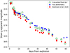 |
Fig. A.1. Comparison of the g-band light curves from this work (blue points), B20 (red points) and B20 converted from their BV magnitudes using the formula from Jester et al. (2005) (green points). |
Appendix B: Determination of the explosion epoch from the light curve modelling
Allowing t0 to vary as a free parameter in the modelling (within a range of ±1 day), we identified the best fit by considering only the first 2.5 days after our first detection, as these data points provide the strongest constraint on the explosion epoch. The resulting time offsets from the assumed explosion epoch (MJD 58845.08) were 0.06 days, −0.3 days, and −0.9 days for the ‘IIb progenitor without CSM,’ ‘IIb progenitor with CSM,’ and ‘stripped progenitor with CSM’ models, respectively. The rising portions of the shifted model light curves, along with the observed Clear band light curve, are shown in Fig. B.1. As discussed in Sect. 5, the model without CSM best reproduces the rising part of the light curve, which is also evident from Fig. B.1. For the other two scenarios, a trade-off was necessary between fitting the early rising part and the later flattened part, as improving the fit for one part negatively impacted the fit for the other. Consequently, we were unable to obtain a good fit for the rising part of the light curve in these two cases. Given that the model without CSM provides the best fit to the rising part of the light curve, the explosion time derived from this model is likely to be more accurate than the other two. This explosion time is also consistent with all other methods discussed in the paper.
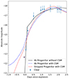 |
Fig. B.1. Comparison of the observed early light curve rise with those of the best-fit models: IIb progenitor model without CSM, and models with CSM for both IIb and stripped progenitors. |
All Tables
Observational facilities and instrumentation used in the photometric follow-up of SN 2018ivc.
All Figures
|
Fig. 1. Colour image of the host galaxy Messier 77 and of SN 2018ivc taken on 2018 November 27, four days after the explosion, with the PROMPT6 telescope. The image is a combination of the frames obtained with the B, V and R filters using the RGB technique. The SN location is marked. |
| In the text | |
|
Fig. 2. Parabolic fit on the fluxes of the three detections of November 23. The explosion is predicted to occur when the curve crosses the zero flux level, at MJD 58445.11. The last upper limit is shown as a downwards triangle. |
| In the text | |
|
Fig. 3. Four stamps of the template-subtracted images from the PROMPT telescopes of 23 November 2018, showing the fast rise of SN 2018ivc after the explosion. Top-left: last non-detection with a threshold of 2.5σ. Top-right: First detection. Bottom-left: second, much brighter detection of the night. Bottom-right: First PROMPT image from the following night, with the source close to maximum light. The colour scales are roughly the same on all the stamps. All the green circles are centred on the position of the transient calculated by the PSF fitting and have a radius of 5″. |
| In the text | |
|
Fig. 4. Open, JC BVRI, Sloan ugriz, ATLAS c, o and NIR JHK light curves (left) over the one-year follow-up of SN 2018ivc. The graph has been broken into two windows (before and after +3 months) for clarity. Downward triangles mark upper limits. B − V and V − R reddening-corrected colour curves (right) of SN 2018ivc (filled points) and of the comparison objects: SNe 1993J, 2001fa, 2007fz, 1996al, and 1998S. For SN 2018ivc, we considered both the low (orange circles) and high (blue diamonds) reddening scenarios (see Sect. 4.4). |
| In the text | |
|
Fig. 5. Comparison of the absolute light curves of SNe 2018ivc, 1993J, 2016gkg (adopting the explosion epoch from Arcavi et al. 2017), KSN2011a, and KSN2011d in the first two days after the explosion. For SN 2018ivc, the Clear (calibrated as r-band) magnitudes are plotted, for SNe 1993J and 2016gkg the V-band and for the two Kepler’s SNe the KP-filter ones. For SN 2018ivc, the error bars are also plotted, summing in quadrature the errors from the photometric measurements, the μ and the internal reddening. Both the low and high host reddening scenarios are considered. The official discovery date of SN 2018ivc is marked with a vertical line. The downward triangles mark the last non-detection of each SN. The absolute r-band light curve following the SBO from a typical Wolf-Rayet model (M = 5 M⊙, R = 10 R⊙, Eexpl = 1 foe) of Nakar & Sari (2010) is also plotted (black line). |
| In the text | |
|
Fig. 6. Spectral sequence of SN 2018ivc, spanning two months of evolution after the discovery. The phases relative to the explosion are reported. The spectra have been corrected for redshift and Milky Way extinction only, as the host galaxy reddening is highly uncertain. The principal identified transitions are highlighted with vertical dashed lines. The possible high velocity feature discussed in Sect. 5.2 is also marked in gray. Each spectrum is shifted by a constant for graphical purposes. The regions most affected by the telluric absorption bands are marked in cyan. |
| In the text | |
|
Fig. 7. Comparison of velocities from Hα in spectra of SNe 1993J, 1996al (considering the blue component of Hα), 2011fu (Kumar et al. 2013), 2011dh (Marion et al. 2014) 2018ivc (this work), and a sample of SNe IIP/IIL (Gutiérrez et al. 2017, using the minimum of the Hα absorption). For SN 2018ivc, the velocity is derived from the position of the minimum of the absorption. |
| In the text | |
|
Fig. 8. Hα line of the +49 d Keck-I/LRIS spectrum of SN 2018ivc published by B20. The rest-frame Hα wavelength is marked and coincides with the narrow Hα emission with a narrow P Cygni profile. The HV feature at 6400 Å is visible on the left side (see Sect. 5.2). A 2m Faulkes/FLOYDS spectrum taken the day before the Keck-I one, also reported in B20, already shows the narrow absorption feature. Our lower-resolution spectra taken near that phase are also shown, in which a ‘small’ emission feature is visible at rest-frame zero velocity. A zoom on the P Cygni feature in the Keck spectrum is plotted in the blow-up box. |
| In the text | |
|
Fig. 9. Comparison of an early spectrum of SN 2018ivc (+10 d) with those at similar epochs of SNe IIn 1996al and 1998S, SNe IIb 1993J and 2011fu, SN IIL 2007fz. The true spectral appearance of SN 2018ivc in the first days is hidden by the effects of interaction. H and He transitions are marked by the continuous and dashed vertical lines, respectively. |
| In the text | |
|
Fig. 10. Archival r-band image from the Dark Energy Survey DR1 of the field of SN 2018ivc. The cross marks the SN position. The field-of-view of VLT+MUSE in narrow-field mode is shown by the square. The H II regions from which we extracted the spectra to evaluate the Balmer decrement are highlighted by the circles. |
| In the text | |
|
Fig. 11. Pseudo-bolometric uBgVrRiIz light curves of SN 2018ivc, for both the low and high reddening scenarios. The inset shows a blow-up of the first two months after the explosion. For reference, we plot also the pseudo-bolometric light curve without any correction for reddening in black; the short plateau feature is more pronounced. The decay slope of 56Co (0.98 mag (100 d)−1) is reported with a dashed purple line for comparison. At late phases (after +100 days) the evolution of SN 2018ivc is close to being powered by the 56Co decay. The systematic error bar due to the uncertainty on the distance is reported in the bottom-left corner. |
| In the text | |
|
Fig. 12. Comparison between the BVRI absolute light curves of SNe 1993J, 2011fu and 2013df (IIb), 1996al (IIn), 2001fa and 2007fz (IIL), and 2018ivc up to 60 days after maximum. For SN 2018ivc, the absolute light curves for both the low and high reddening scenarios are plotted with circles and squares, respectively. SN 2007fz presents a well-defined secondary peak between one and two weeks after maximum, while SN 2018ivc shows a short plateau. The two objects have quite similar photometric evolution. |
| In the text | |
|
Fig. 13. Histogram of the distribution of the average flux ratio Hα/He I λ5876 in three SNe IIb (SNe 1993J, 2011fu and 2013df, in blue), nine SNe IIL from Faran et al. (2014) (in red) and SN 2018ivc (in green) between one and three months after the explosion. The majority of SNe IIL have a Hα/He I λ5876 ratio of around 7, with some outliers, while SNe IIb have a ratio between 2 and 3. With a ratio of 8.4, SN 2018ivc would be a type IIL SN. |
| In the text | |
|
Fig. 14. Comparison of the late mean spectrum of SN 2018ivc (+52 d) with those of some reference types IIL and IIb SNe, taken at late phases. The sample includes: SNe 1993J, 2011fu and 2013df (Shivvers et al. 2019) for type IIb, SNe 2001fa and 2007fz (Faran et al. 2014) for type IIL. SNe IIL have strong Hα and faint or no He I lines, the opposite is true for SNe IIb. Hα and the principal He I lines are marked by the vertical continuous and dashed lines, respectively. |
| In the text | |
|
Fig. 15. Zoom on the HV feature on the blue side of Hα in the rest-frame velocity. The velocity of the feature clearly slows down with the phase. |
| In the text | |
|
Fig. 16. Models evolved from the progenitor without adding CSM. The top panel displays the best fit model of the first 20 days of BVRIi and Clear light curves of SN 2018ivc. The bottom panel shows the photospheric velocity corresponding to the best fit model along with the observed photospheric velocity. |
| In the text | |
|
Fig. 17. Density profile attached to the progenitor. The inset shows a zoom-in of the intermediate component (‘INT’) attached between the progenitor and the CSM. |
| In the text | |
|
Fig. 18. Effect of nCSM on the rise of the Clear band light curve. Increasing the value of nCSM resulted in steeper light curves. |
| In the text | |
|
Fig. 19. First 20 days of the BVRIi and Clear band model light curves corresponding to the ‘stripped_6M’ model along with the observed multi-band light curves of SN 2018ivc (top). Photospheric velocity evolution corresponding to these models along with the observed photospheric velocity (bottom). |
| In the text | |
|
Fig. 20. Density profile attached to the stripped progenitor. The inset shows a zoom-in of the CSM profile attached. |
| In the text | |
|
Fig. 21. Model light curves corresponding to the three stripped models of the first 20 days of Clear band of SN 2018ivc along with the observed Clear band light curves (top). Photospheric velocity evolution corresponding to these models along with the observed photospheric velocity (bottom). |
| In the text | |
|
Fig. 22. Best fit model with the addition of CSM. The top panel features the best fit model of the first 20 days of BVRIi and Clear light curves of SN 2018ivc along with the observed multi-band light curves. The bottom panel shows the photospheric velocity evolution corresponding to the best fit model along with the observed photospheric velocity. |
| In the text | |
|
Fig. A.1. Comparison of the g-band light curves from this work (blue points), B20 (red points) and B20 converted from their BV magnitudes using the formula from Jester et al. (2005) (green points). |
| In the text | |
|
Fig. B.1. Comparison of the observed early light curve rise with those of the best-fit models: IIb progenitor model without CSM, and models with CSM for both IIb and stripped progenitors. |
| In the text | |
Current usage metrics show cumulative count of Article Views (full-text article views including HTML views, PDF and ePub downloads, according to the available data) and Abstracts Views on Vision4Press platform.
Data correspond to usage on the plateform after 2015. The current usage metrics is available 48-96 hours after online publication and is updated daily on week days.
Initial download of the metrics may take a while.