| Issue |
A&A
Volume 692, December 2024
|
|
|---|---|---|
| Article Number | A187 | |
| Number of page(s) | 14 | |
| Section | Catalogs and data | |
| DOI | https://doi.org/10.1051/0004-6361/202450758 | |
| Published online | 12 December 2024 | |
Millisecond pulsars phenomenology under the light of graph theory
1
Institute of Space Sciences (ICE, CSIC), Campus UAB, Carrer de Can Magrans s/n,
08193
Barcelona,
Spain
2
Institut d’Estudis Espacials de Catalunya (IEEC),
08034
Barcelona,
Spain
3
INAF – Osservatorio Astronomico di Roma,
Via Frascati 33,
00078
Monte Porzio Catone (RM),
Italy
4
Tor Vergata University of Rome,
Via della Ricerca Scientifica 1,
00133
Roma,
Italy
5
Sapienza Università di Roma,
Piazzale Aldo Moro 5,
00185
Rome,
Italy
6
Institució Catalana de Recerca i Estudis Avançats (ICREA),
08010
Barcelona,
Spain
7
INAF – Osservatorio Astronomico di Capodimonte,
Salita Moiariello 16,
80131
Naples,
Italy
★ Corresponding author; This email address is being protected from spambots. You need JavaScript enabled to view it.
Received:
17
May
2024
Accepted:
16
October
2024
Abstract
We compute and apply the minimum spanning tree (MST) of the binary millisecond pulsar population, and discuss aspects of the known phenomenology of these systems in this context. We find that the MST effectively separates different classes of spider pulsars – eclipsing radio pulsars in tight binary systems with a companion of either ~0.1–0.8 M⊙ (redbacks) or ≲0.06 M⊙ in mass (black widows) – into distinct branches. The MST also separates black widows (BWs) in globular clusters from those found in the field and groups other pulsar classes of interest, including transitional millisecond pulsars (tMSPs). Using the MST and a defined ranking for similarity, we identify possible candidates likely to belong to these pulsar classes. In particular, based on this approach, we propose the BW classification of J1300+1240, J1630+3550, J1317−0157, J1221−0633, J1627+3219, J1737−0314A, and J1701−3006F, discuss that of J1908+2105, and analyze J1723−2837, J1431−4715, and J1902−5105 as possible transitional systems. We introduce an algorithm that quickly locates where new pulsars fall within the MST and use this to examine the positions of the TMSP IGR J18245−2452 (PSR J1824−2452I), the tMSP candidate 3FGL J1544.6−1125, and the accreting millisecond X-ray pulsar SAX J1808.4−3658. Assessing the positions of these sources in the MST – assuming a range for their unknown variables (e.g., the spin period derivative of PSR J1824−2452I) –, we can effectively narrow down the parameter space necessary for searching for and determining key pulsar parameters through targeted observations.
Key words: catalogs / binaries: general / stars: neutron
© The Authors 2024
 Open Access article, published by EDP Sciences, under the terms of the Creative Commons Attribution License (https://creativecommons.org/licenses/by/4.0), which permits unrestricted use, distribution, and reproduction in any medium, provided the original work is properly cited.
This article is published in open access under the Subscribe to Open model. This email address is being protected from spambots. You need JavaScript enabled to view it. to support open access publication.
1 Introduction
This article continues the study that integrates principal component analysis (PCA; e.g., Pearson 1901; Shlens 2014) and the application of graph theory (e.g. Wilson 2010) into the field of pulsar astrophysics (see, e.g., Maritz et al. 2016; García et al. 2022; García & Torres 2023; Vohl et al. 2024). PCA is a dimensionality-reduction technique suitable for pinpointing the variables that contain most of the variance of a sample (see, e.g., Cassanelli et al. 2022). Graph theory provides a robust theoretical framework whose objects – the graphs – represent pulsars and their variables. Here, we specifically consider the population of millisecond pulsars (MSPs), weakly magnetized and rotating neutron stars with spin periods shorter than 10 ms. These objects are usually hosted in tight binary systems with a lowmass (<1 M⊙) companion star. MSPs offer unique insights into stellar evolution, the interaction between magnetic fields and plasma transferred by the donor star, and particle acceleration from compact objects, particularly in binary systems (see, e.g., Manchester 2017; Papitto & Bhattacharyya 2022 for reviews).
By treating each MSP as a node, we compute the minimum spanning tree (MST; see e.g., Kruskal 1956; Gower & Ross 1969) of the MSP population, and use it both to describe the population as a whole and to identify individual pulsars that may warrant further investigation due to their unique attributes or positions within the graph.
We specifically examine locations in the MST in which we find spider pulsars (see, e.g., Eichler & Levinson 1988; Roberts 2013; Roberts et al. 2018; Di Salvo et al. 2023), which are eclipsing radio pulsars in tight binary systems. These spider pulsars can be separated into redbacks (RBs), which have a non-degenerate main sequence companion with a mass in the range of ~0.1–0.8 M⊙, and BWs, which have a ≲0.06 M⊙ semidegenerate companion. We also consider tMSPs (Papitto & de Martino 2022), which exhibit dramatic state changes, going from rotation-powered – where they behave as RBs – to accretion-powered and vice versa on timescales as short as a few weeks. Driven by the method developed by García & Torres (2023), which allows an MST to be divided into distinct parts based on specific variables, we explore how to classify MSPs into different groups. Finally, we use the algorithms described below to search for the positions of pulsars within the graph – specifically focusing on those whose properties have not been measured – to predict ranges for specific variables and their characteristic phenomenology.
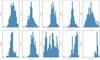 |
Fig. 1 Distribution of the logarithm of the ten variables considered for the sample of 218 pulsars. |
2 The sample variance and the MST
2.1 Sample selection
The sample used is taken from the most recent version of the Australia Telescope National Facility (ATNF) catalog, v2.1.1 (Manchester et al. 2005), imposing that pulsars have a spin period in the millisecond range (P < 10−2 s) and a positive spin period derivative (![Mathematical equation: $\[\dot{P}\]$](/articles/aa/full_html/2024/12/aa50758-24/aa50758-24-eq1.png) > 0 s s−1). The latter allows us to calculate the intrinsic variables derived from P and
> 0 s s−1). The latter allows us to calculate the intrinsic variables derived from P and ![Mathematical equation: $\[\dot{P}\]$](/articles/aa/full_html/2024/12/aa50758-24/aa50758-24-eq2.png) as described in Sect. 2.2. A total of 218 pulsars result from these cuts. Of these, 43 are confirmed as BWs, 9 of which are in globular clusters (see e.g., Swihart et al. 2022; Koljonen & Linares 2023; Freire et al. 2017; Lynch et al. 2012; Douglas et al. 2022), 16 are confirmed as RBs, 2 of which are in globular clusters (see e.g., Strader et al. 2019; Koljonen & Linares 2023), and 2 are confirmed as tMSPs, J1023+0038 (Archibald et al. 2009) and J1227−4853 (Bassa et al. 2014). We note that tMSP J1824−2452I (Eckert et al. 2013) is excluded from the sample as it does not have a
as described in Sect. 2.2. A total of 218 pulsars result from these cuts. Of these, 43 are confirmed as BWs, 9 of which are in globular clusters (see e.g., Swihart et al. 2022; Koljonen & Linares 2023; Freire et al. 2017; Lynch et al. 2012; Douglas et al. 2022), 16 are confirmed as RBs, 2 of which are in globular clusters (see e.g., Strader et al. 2019; Koljonen & Linares 2023), and 2 are confirmed as tMSPs, J1023+0038 (Archibald et al. 2009) and J1227−4853 (Bassa et al. 2014). We note that tMSP J1824−2452I (Eckert et al. 2013) is excluded from the sample as it does not have a ![Mathematical equation: $\[\dot{P}\]$](/articles/aa/full_html/2024/12/aa50758-24/aa50758-24-eq3.png) measurement, although it is analyzed in Sect. 4.1. These pulsars are listed in Table A.1.
measurement, although it is analyzed in Sect. 4.1. These pulsars are listed in Table A.1.
According to the third pulsar catalog by the Fermi Large Area Telescope (Fermi-LAT, see Smith et al. 2023), 103 pulsars out of the 218 of our sample are gamma-ray emitters.
2.2 Variables and PCA
Figure 1 shows the logarithmic distribution of the spin period (P) and the spin period derivative (![Mathematical equation: $\[\dot{P}\]$](/articles/aa/full_html/2024/12/aa50758-24/aa50758-24-eq4.png) ), the surface magnetic flux density (Bs), the magnetic field at the light cylinder (Blc), the spin-down energy loss rate (
), the surface magnetic flux density (Bs), the magnetic field at the light cylinder (Blc), the spin-down energy loss rate (![Mathematical equation: $\[\dot{E}\]$](/articles/aa/full_html/2024/12/aa50758-24/aa50758-24-eq5.png) sd), the surface electric voltage (ΔΦ), the Goldreich–Julian charge density (ηGJ), the binary period (PB), the projected semi-major axis of the orbit (A1), and the median mass of the companion star for each system (MC). We do not consider the characteristic age (τc = P/2
sd), the surface electric voltage (ΔΦ), the Goldreich–Julian charge density (ηGJ), the binary period (PB), the projected semi-major axis of the orbit (A1), and the median mass of the companion star for each system (MC). We do not consider the characteristic age (τc = P/2 ![Mathematical equation: $\[\dot{P}\]$](/articles/aa/full_html/2024/12/aa50758-24/aa50758-24-eq6.png) ) here, because in binary systems additional torques imparted on the pulsar during accretion phases can render this estimate unreliable (see, e.g., Kiziltan & Thorsett 2010; Tauris et al. 2012; Jiang et al. 2013). The distributions are not normal (which is also the case for the set of distributions of the original variables, without logarithm), and so we use the robust scaler to scale them (subtract the median and divide by the interquartile range; see, for example, de Amorim et al. 2022). Figure 2 shows how the PB, A1, and MC distribution can be used to distinguish BWs from other classes. However, when none of these variables are used in the analysis, the distinction is no longer evident, and spider pulsars are seen as a more homogeneous group.
) here, because in binary systems additional torques imparted on the pulsar during accretion phases can render this estimate unreliable (see, e.g., Kiziltan & Thorsett 2010; Tauris et al. 2012; Jiang et al. 2013). The distributions are not normal (which is also the case for the set of distributions of the original variables, without logarithm), and so we use the robust scaler to scale them (subtract the median and divide by the interquartile range; see, for example, de Amorim et al. 2022). Figure 2 shows how the PB, A1, and MC distribution can be used to distinguish BWs from other classes. However, when none of these variables are used in the analysis, the distinction is no longer evident, and spider pulsars are seen as a more homogeneous group.
Figure 3 shows the results of the PCA analysis applied to these variables. In the left panel of Fig. 3, we observe how most of the variance is distributed in the first two principal components (PCs). Likewise, the central panel shows that the whole variance is represented in four-dimensional space, that is, we need the first four PCs to cover 100% of the variance of the sample. This relatively low number of PCs results from the fact that within the dipolar model used as a proxy (see, e.g., Lorimer & Kramer 2012), all physical variables depend on P and ![Mathematical equation: $\[\dot{P}\]$](/articles/aa/full_html/2024/12/aa50758-24/aa50758-24-eq7.png) , and also that A1 of a binary system is related to the PB and the MC (in this case through the total mass of the system, i.e., the sum of the masses of the pulsar and its companion) via Kepler’s third law. The PCA, as shown in the right panel of Fig. 3, does not highlight the dominant influence of key variables for the separation between pulsar spiders, such as the MC, but provides a more complex classification where its dominance is balanced with other variables. More specifically, the four PCs needed to describe the entirety of the variance have similarly large loadings in several variables (see the right panel of Fig. 3).
, and also that A1 of a binary system is related to the PB and the MC (in this case through the total mass of the system, i.e., the sum of the masses of the pulsar and its companion) via Kepler’s third law. The PCA, as shown in the right panel of Fig. 3, does not highlight the dominant influence of key variables for the separation between pulsar spiders, such as the MC, but provides a more complex classification where its dominance is balanced with other variables. More specifically, the four PCs needed to describe the entirety of the variance have similarly large loadings in several variables (see the right panel of Fig. 3).
2.3 Minimum spanning tree
Kruskal (1956), Kleinberg & Tardos (2005) and Erickson (2019) explain the necessary concepts to calculate an MST. We refer the reader to these references for details. We define a Euclidean distance over the variables or the PCs described above, as using the first four PCs (~100% of the explained variance) produces the same MST as when using all variables (and thus the results from the analysis that follows from the graph are the same), but is less demanding given the reduced dimensionality of the problem. With this Euclidean distance, we first compute a complete, undirected, and weighted graph G(V, E) = G(218, 23 653), with |V|1=218 nodes and |E| = 23 653 edges, with a specific weight value defining each edge. From that, we obtain the MST of this sample, T(V, E′) = (218, 217), with |V| = 218 nodes and |E′| = 217 edges, as shown in Fig. 4.
The MST can separate BWs from RBs, with tMSPs appearing close to each other, in the same structure, as shown in Fig. 4. A zoom onto these tree regions is shown in Fig. 5, where several pulsars are highlighted; these are discussed below. We provide an online tool2 to allow the reader to zoom into, identify, and mark different portions of the MST for further study.
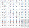 |
Fig. 2 Cross-dependence of the ten variables considered. Confirmed BWs (in red) and RBs (in green) are separately noted. For visualization reasons, no distinction is made between MSPs residing in globular clusters and those not, and the tMSPs are marked in green due to their behavior as RBs. The pulsars not yet assigned to any of these classes are shown in blue. The main diagonal shows the distribution for each variable. The panels with the shaded background show the pairs formed with PB, MC, and A1, which best differentiate the BWs from the rest. |
 |
Fig. 3 PCA results for the logarithm of the set of variables for the whole population of 218 MSPs. The left panel, also called the scree plot, shows the explained variance of each PC according to the eigenvalues of the covariance matrix. We note that the covariance matrix calculates the relationships between pairs of variables, showing how changes in one variable are associated with changes in another. It represents the amount of information contained in each PC. The central panel shows the cumulative explained variance by the new variables defined through the PCA analysis. The right panel shows the “weight” (also called loading) that each variable has concerning each PC, indicating its contribution to the variance captured by that PC. This value is the coefficient held in each eigenvector of the covariance matrix. Negative values imply that the variable and the PC are negatively correlated. Conversely, a positive value shows a positive correlation between the PC and the variable. |
 |
Fig. 4 Minimum spanning tree of the binary pulsar population defined as T(218, 217) based on the complete, undirected, and weighted graph G(218, 23 653) computed from the Euclidean distance among ten scaled variables (or the equivalent four PCs that describe their whole variance). Each node in the MST represents a pulsar. The MST separately notes confirmed BWs (red), RBs (green), and tMSPs J1023+0038 and J1227−4853 (yellow), respectively. Also, the BWs and RBs in globular clusters (light red and light green, respectively) are highlighted. The RBs J1622−0315 (green) and the RB candidate J1302−3258 (light teal) are also noted in the rightmost branch of the MST. The unclassified ones appear in blue. See Table A.1 for more details. |
2.3.1 Black widow pulsars in the graph
We now focus on some specific pulsars (see Fig. 5). Two of these are J1300+1240 and J1630+3550, which have not yet been explicitly classified as BWs but have been discussed by Yan et al. (2013), Sobey et al. (2022). A possible formation scenario for J1300+1240, suggested by Yan et al. (2013), is in low-mass, narrow-orbit bound binaries. Here, the initial point of departure is a low-mass binary pulsar with a very narrow orbit, such as the known BW J1959+2048. Because its velocity and rotation period are comparable to those of J1959+2048, J1300+1240 may evolve in this scenario. J1630+3550 is an MSP in a binary system of 7.6 h orbiting a companion with a minimum mass of 0.0098 M⊙. These parameters can indicate a BW, as stated in Lewis et al. (2023). From the MST graph, we can see that they are located in the BW region. We can further support their potential categorization as BWs by observing the ranking of the nearest pulsars based on the Euclidean distance derived from the defined variables, which can be obtained using the online tool we provide with this paper. We note that the ranking simply provides a distance-ordered list of one pulsar relative to all others, while the MST provides a global way to connect all pulsars considering all distances, optimizing the total path. Only the nearest neighbor to any given pulsar will have an immediately recognized position within the MST; as such, the nearest neighbor will always be one of the pulsars connected to the pulsar of interest in the MST. For a more detailed discussion and examples regarding the differences between the ranking and the MST, see García et al. (2022). Nine of the ten nearest neighbors of J1300+1240 have already been classified as BWs, and the remaining object is J1630+3550, whose ten nearest neighbors are BWs.
Among the interesting sources highlighted in Fig. 5 are J1317−0157 and J1221−0633, which were classified as BW systems by Swiggum et al. (2023); they have tight orbits, low-mass companions, and exhibit eclipses. In both cases, their nearest neighbor ranking contains nine confirmed BWs, with the exception being J1627+3219.
In this regard, the position of J1627+3219 in the MST, underscored by its ranking, where eight of its ten nearest neighbors are confirmed BW pulsars, supports its categorization in this group. This assertion is further bolstered by the findings of Braglia et al. (2020), who identified a candidate optical periodicity, necessitating verification through subsequent observations. Recent research by Corcoran et al. (2023) also underscores the potential BW nature of this pulsar. Still, the lack of detected radio pulsations highlights the need for further studies to fully understand its nature.
We also pinpoint J1737−0314A, which, according to the timing solution provided by Pan et al. (2021), is likely a BW system. Looking at its ranking, its categorization as a BW is favored, as it contains nine confirmed BWs among its ten nearest neighbors, the remaining one being J1701−3006F. In addition, this latter source, considering its mass limit and orbital features, is also favored to be a BW, as outlined in Freire et al. (2005); although eclipses have not been observed, this absence could be due to a low orbital inclination (Vleeschower et al. 2024). On the other hand, its nearest neighbor ranking shows six BWs, with the closest being J1701−3006E; see also King et al. (2005). We note that both J1701−3006E and J1701−3006F appear connected in the MST (see Fig. 5), filling the end of a branch that contains a large number of these cases.
The position of J1555−2908 in the MST, being the only confirmed BW away from the rest, is noteworthy. Kennedy et al. (2022) performed an extensive analysis using optical spectroscopy and photometry. This study, combined with γ-ray pulsation timing information alongside a companion mass of 0.06 M⊙, concluded that J1555−2908 lies at the observed upper boundary of what is typically classified as a BW system. We note that its nearest neighbor, J1835−3259B, is not a BW. Of interest to all sources discussed in this section, we note that no other non-BW pulsar – except J1908+2105, which is discussed in the following section – has more than five confirmed BWs in its ranking.
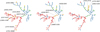 |
Fig. 5 Zoom onto the leftmost part of the MST shown in Fig. 4. The locations of the pulsars (shown in orange) discussed in Sect. 2.3.1 (left panel), Sect. 2.3.2 (central panel), and Sect. 2.3.3 (right panel) can be seen more clearly here. The same color code is used as in Fig. 4, where the confirmed BWs appear in red, RBs in green, tMSPs in yellow, and the BWs and RBs in globular clusters are shown in light red and light green, keeping the unclassified pulsars in blue. |
2.3.2 Redbacks pulsars in the graph
Figure 5 shows that RB pulsars do not appear clustered like BWs, but are mostly close to each other, with a small fraction near the border of BWs. The caveat here is the smaller number of RBs known so far.
The pulsar J1908+2105 is an interesting case within the RB class. This one is right on the frontier with the part of the MST mostly populated by BWs and could be classified as such, especially given its minimum companion mass of 0.06 M⊙ and its short PB of 0.14 days (Strader et al. 2019). However, the pronounced radio eclipses of this system align it more closely with RBs (also see, e.g., Koljonen & Linares 2023; Deneva et al. 2021). We note that the ranking of the ten nearest neighbor pulsars to J1908+2105 shows that eight of them are BWs. The fifth and ninth pulsars in the ranking, J2039−5617 and J0337+1715 respectively, are RB and an uncategorized pulsar. This situation, where the ranking of a given pulsar thought to pertain to one class (RB) is dominated by pulsars belonging to the other, only arises in the case mentioned above. Thus, the MST location and the ranking favor a BW classification for J1908+2105 – or at the very least do not rule out.
On the other hand, the gamma-ray source 3FGLJ2039−5617 (PSR J2039−5617) is almost certainly associated with an optical binary that is listed as an RB candidate by Strader et al. (2019). Its predicted nature as an RB is validated by Corongiu et al. (2021), who found clear evidence of eclipses of the radio signal for about half of the orbit, which they associate with the presence of intrabinary gas. J2039−5617 appears as a confirmed RB in Koljonen & Linares (2023). Furthermore, it shares similarities with the confirmed RB J2339−0533, exhibiting a peak in gamma-ray emission close to a minimum in its optical emission, which contrasts with the expected phase of the intrabinary shock (IBS) as seen in An et al. (2020). This similarity between J2039−5618 and J2339−0533 and their position in the MST highlight intriguing aspects of their behavior, which merit further analysis.
The distinct positions of J1622−0315, J1302−3258 (see Fig. 4 for the location of the latter two in the MST), and J1628−3205, located far from the rest of the RBs in the MST, also capture our attention. J1622−0315 is one of the lightest known RB systems, with a companion mass of 0.15 M⊙, and a relatively hot companion (Yap et al. 2023; Sen et al. 2024). This system is notable for its PB of 0.16 days, which is marginally smaller than those of other RBs, which typically have a PB of 0.2 days or more.
On the other hand, J1302−3258 is classified as an RB candidate and is reported to have a minimum companion mass of 0.15 M⊙ (Strader et al. 2019). However, it is distinguished by the absence of an identified optical companion and lacks published evidence of extensive radio eclipses. Koljonen & Linares (2023) note that, unlike most known RBs and candidates, J1302−3258 does not have a Gaia counterpart, a trend more typical of BWs, which generally possess cooler companion stars with fainter optical magnitudes. J1628−3205 is a RB in a 0.21 day orbit and has a 0.17–0.24 M⊙ companion star (Ray et al. 2012; Li et al. 2014; Strader et al. 2019). Its optical counterpart shows two peaks per orbital cycle. This shape is reminiscent of the ellipsoidal deformation of a star that nearly fills its Roche-lobe in a high-inclination binary, and suggests that heating by the pulsar wind is not a major effect. In this context, J1628−3205 is an intermediate case among RBs, falling between systems where the companion star’s emission is dominated by pulsar irradiation (e.g., J1023+0038) and those where it is not (e.g., J1723−2837, J1622−0315, J1431−4715)(see Li et al. 2014; Yap et al. 2023; de Martino et al. 2024 and references therein).
2.3.3 Transitional pulsars in the graph
The pulsars J1723−2837, J1902−5105, and J1431−4715 appear in the same part of the MST as the known tMSPs J1227−4853 and J1023+0038 (Fig. 5), and are also the only ones in the sample containing at least one known tMSP in their top three neighbors; see Table 1. The closest neighbors of the two known tMSPs are also shown in Table 1.
J1723−2837 is a nearby (d ~ 1 kpc based on Gaia parallax measure) 1.86 ms RB in a binary system with a 15 h period (Crawford et al. 2013). With an X-ray luminosity of 1032 erg s−1, it ranks among the brightest RBs in that band (see, e.g., Lee et al. 2018). Based on the similarity with the X-ray output of tMSPs in the rotation-powered pulsar state, Linares (2014) suggested that it is one of the most likely candidates to offer the opportunity to observe a transition to an accretion state. The observed emission in both soft (Bogdanov et al. 2014; Hui 2014) and hard X-rays (Kong et al. 2017) is modulated at the PB, indicative of an origin in the IBS between the pulsar wind and mass outflow from the companion star. On the other hand, its optical counterpart shows no sign of significant irradiation, with two peaks per orbital cycle (Li et al. 2014).
J1902−5105 is a 1.74 ms radio MSP in a binary system with a period of 2 days. It was discovered within the Parkes telescope surveys targeting unidentified Fermi-LAT sources (Kerr et al. 2012). It is a relatively bright MSP located at a distance of ~1.2 kpc (Camilo et al. 2015). It was suggested that the companion is a 0.2–0.3 M⊙ white dwarf with a helium core (Camilo et al. 2015).
Finally, J1431−4715, discovered in the High Time Resolution Universe (HTRU) survey with the Parkes radio telescope is an RB MSP with a P of 2.01 ms in a 10.8 hr orbit with a companion mass of 0.20 M⊙ (Bates et al. 2015; Miraval Zanon et al. 2018; de Martino et al. 2024).
One of the most efficient ways to identify candidate tMSPs is to search for the peculiar variability in the X-ray emission between two intensity levels (known as “high” and “low” modes), which has been observed in all three of the confirmed tMSPs in the so-called subluminous disk state (see, e.g., Patruno et al. 2014; de Martino et al. 2013; Archibald et al. 2015; Papitto et al. 2013; Linares et al. 2014; Bogdanov et al. 2015; Papitto et al. 2019; Baglio et al. 2023; Papitto & de Martino 2022). This method has proven successful in identifying a few candidates (see, e.g., Coti Zelati et al. 2019; Bogdanov & Halpern 2015). However, a methodology for identifying candidates among the radio-emitting pulsars out of the subluminous disk state has yet to be determined. The MST can contribute to this.
Although J1723−2837, J1902−5105, and J1431−4715 are currently detected as radio MSPs and are therefore not expected to exhibit the typical bimodality in the X-ray light curve, we analyzed XMM-Newton archival observations of these sources (ObsID 0653830101 for J1723−2837, ObsID 0841920101 for J1902−5105, and ObsID 0860430101 for J1431−4715) to check for possible mode switching. We confirm the absence of moding in our analysis; see Appendix C. This implies a lack of conclusive evidence regarding the transitional nature of J1723−2837, J1902v5105, and J1431−4715, but their position in the MST and their neighbor ranking confirm them as subjects of interest as potential transitional systems, though currently in the radio pulsar state. The relative proximity of J1723−2837 and particularly J1902−5105 renders them optimal candidates for potentially unveiling a future transition from a rotation-powered state to an accretion-powered one.
Ranking of the nodes in the tMSPs region in the MST.
3 MST clustering
Here we apply a clustering algorithm designed to separate an MST into different parts following a quantitative prescription. We describe the methodology in Appendix B. Figure 6 shows separated branches, and Fig. 7 shows the distributions for each magnitude considering them. This is how the MST visually represents the binary MSP population, with no prior assumption on the nature of the nodes.
Two of the branches indicated by the method in Fig. 6 (depicted in dark green and pink) contain all of the BWs except for J1555−2908, which was already deemed as lying at the edge of the BW population as discussed in Sect. 2.3.1. In addition, one of these branches (pink) contains most of the candidate or confirmed BWs seen in globular clusters. The BWs in globular clusters together with the rest of the pulsars seen in the pink branch show ![Mathematical equation: $\[\dot{P}\]$](/articles/aa/full_html/2024/12/aa50758-24/aa50758-24-eq8.png) and
and ![Mathematical equation: $\[\dot{E}\]$](/articles/aa/full_html/2024/12/aa50758-24/aa50758-24-eq9.png) values that are generally higher than those of the others; see Fig. 7. We note that these values cannot be reliably measured in a globular cluster due to the acceleration in the cluster gravity well. Similarly, tMSPs and most of the RBs fall into another branch (depicted in gray in Fig. 6). As we see in Fig. 7, pulsars in the orange branch exhibit PB, MC, and A1 values close to those of the pulsars in the gray branch. However, in contrast, they show a lower
values that are generally higher than those of the others; see Fig. 7. We note that these values cannot be reliably measured in a globular cluster due to the acceleration in the cluster gravity well. Similarly, tMSPs and most of the RBs fall into another branch (depicted in gray in Fig. 6). As we see in Fig. 7, pulsars in the orange branch exhibit PB, MC, and A1 values close to those of the pulsars in the gray branch. However, in contrast, they show a lower ![Mathematical equation: $\[\dot{P}\]$](/articles/aa/full_html/2024/12/aa50758-24/aa50758-24-eq10.png) and thus a smaller Bs. The rest of the population, particularly those nodes in the dark blue and brown branches, which are more similar to each other, are markedly different from the other groups, as shown in Table B.1. Figure 7 shows that although these nodes are less obviously separated in the usual representations, such as the typical (P,
and thus a smaller Bs. The rest of the population, particularly those nodes in the dark blue and brown branches, which are more similar to each other, are markedly different from the other groups, as shown in Table B.1. Figure 7 shows that although these nodes are less obviously separated in the usual representations, such as the typical (P, ![Mathematical equation: $\[\dot{P}\]$](/articles/aa/full_html/2024/12/aa50758-24/aa50758-24-eq11.png) )-diagram, they show larger PB, MC, P, and smaller
)-diagram, they show larger PB, MC, P, and smaller ![Mathematical equation: $\[\dot{E}\]$](/articles/aa/full_html/2024/12/aa50758-24/aa50758-24-eq12.png) than the BW pulsars.
than the BW pulsars.
Based on the distributions of the variables seen in the main diagonal of Fig. 7, we can discuss the differences between branches. We see that MC shows sharp distributions around similar values, except for the (pink) branch, which mostly contains BWs in globular clusters, for which MC shows smaller values. The dark green branch, heavily populated by BWs, displays a wider distribution, always within small values. This is reflected in A1 and PB, where the behavior is similar even with somewhat wider distributions, mainly for the branches that do not contain BWs. The widest distributions are observed in P, for all branches but the one depicted in orange – which has a high density of cases around low values. The dark blue branch contains the pulsars with the longest periods. The ![Mathematical equation: $\[\dot{P}\]$](/articles/aa/full_html/2024/12/aa50758-24/aa50758-24-eq13.png) shows different trends for some branches. The orange, brown, and dark blue branches, show sharp behaviors that allow us to more clearly delimit the pulsars they contain, most of which are not classified as BWs or RBs. This is reflected in
shows different trends for some branches. The orange, brown, and dark blue branches, show sharp behaviors that allow us to more clearly delimit the pulsars they contain, most of which are not classified as BWs or RBs. This is reflected in ![Mathematical equation: $\[\dot{E}\]$](/articles/aa/full_html/2024/12/aa50758-24/aa50758-24-eq14.png) , ηGJ, Blc, and Bs; branches containing BWs and RBs show a wider distribution, shifted toward larger values for the dark green, gray, and pink branches, considering that the latter two contain different types of spider pulsars. In addition, Fig. 7 can be compared with Fig. 2. The former is more informative, as the clustering technique separates the nodes into groups that are significantly different from one another (see Table B.1), beyond the known RBs and RBs.
, ηGJ, Blc, and Bs; branches containing BWs and RBs show a wider distribution, shifted toward larger values for the dark green, gray, and pink branches, considering that the latter two contain different types of spider pulsars. In addition, Fig. 7 can be compared with Fig. 2. The former is more informative, as the clustering technique separates the nodes into groups that are significantly different from one another (see Table B.1), beyond the known RBs and RBs.
In closing this section, we note that the MST technique orders the pulsars according to one or several of the variables considered (this was discussed at length already in the first work of this series by García et al. 2022 for the whole pulsar population). Figure 8 below serves as an example (data that can be used to construct similar figures for other paths are provided in the online tool that accompanies this paper) of how the variables are ordered along a given sequence of consecutive nodes (or path). Figure 8 shows the values of P, ![Mathematical equation: $\[\dot{P}\]$](/articles/aa/full_html/2024/12/aa50758-24/aa50758-24-eq15.png) , Bs,
, Bs, ![Mathematical equation: $\[\dot{E}\]$](/articles/aa/full_html/2024/12/aa50758-24/aa50758-24-eq16.png) , MC, A1, and PB along a path in the MST.
, MC, A1, and PB along a path in the MST.
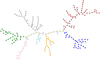 |
Fig. 6 Minimum spanning tree of the MSP population is defined as T(218, 217), separated into significant branches according to the algorithm described in the text (see Sect. 3). The branches group a comparable number of pulsars: gray (39), orange (20), dark blue (31), brown (54), dark green (30), and pink (16). The trunk (in dark khaki) has only 14 nodes, with 14 others (in sky blue) that are not considered to pertain to any significant branch or trunk and appear to be the noise of the former structures. |
4 Localizing a new node
We introduce an incremental algorithm for updating the MST when new nodes are considered. This can be used to infer where a new node with given properties will fall in the MST. In practice, when we add a new node and compute its distance from all other nodes in the graph, we preserve the known distances among the previously existing nodes. In this process, we keep the scaling of the distance used in the calculation of the original MST, denoted T, to which the new node will be added. This involves identifying potential cycles that would be formed with existing T, adding new edges, and discarding them so that the resulting graph remains an MST. This approach, while avoiding the complete recalculation of the MST, delivers the location of the new node concerning the former ones, leading to an updated T, which we refer to as T′. This process follows the principles outlined in traditional graph theory; e.g., the correctness of Prim’s algorithm according to the MST theorem, and the MST lemma as the cycle property (see, e.g., Prim 1957; Wilson 2010; Roughgarden 2019).
4.1 IGR J18245−2452—PSR J1824−2452I
As tMSP IGR J18245−2452 (or PSR J1824−2452I; see, e.g., Papitto et al. 2013) lacks a measured value of ![Mathematical equation: $\[\dot{P}\]$](/articles/aa/full_html/2024/12/aa50758-24/aa50758-24-eq17.png) , it is initially excluded from the sample used in this work (see Sect. 2.1). Considering its measured values for P, PB, MC, and A1, we assume a value for the
, it is initially excluded from the sample used in this work (see Sect. 2.1). Considering its measured values for P, PB, MC, and A1, we assume a value for the ![Mathematical equation: $\[\dot{P}\]$](/articles/aa/full_html/2024/12/aa50758-24/aa50758-24-eq18.png) and add this pulsar to T in Fig. 4. Based on the estimated Bs ~ (0.7–35) × 108 G by Ferrigno et al. (2014), and its known P, we can compute3 a range of
and add this pulsar to T in Fig. 4. Based on the estimated Bs ~ (0.7–35) × 108 G by Ferrigno et al. (2014), and its known P, we can compute3 a range of ![Mathematical equation: $\[\dot{P}\]$](/articles/aa/full_html/2024/12/aa50758-24/aa50758-24-eq19.png) ~ (1.2 × 10⁻²¹−3 × 10⁻¹⁸) ss−1. We take ten equispaced values in this range (and their concurrent values of all physical variables derived taking
~ (1.2 × 10⁻²¹−3 × 10⁻¹⁸) ss−1. We take ten equispaced values in this range (and their concurrent values of all physical variables derived taking ![Mathematical equation: $\[\dot{P}\]$](/articles/aa/full_html/2024/12/aa50758-24/aa50758-24-eq20.png) into account), and we construct for each one a T′.
into account), and we construct for each one a T′.
When we assume the lowest values of the given range, ![Mathematical equation: $\[\dot{P}\]$](/articles/aa/full_html/2024/12/aa50758-24/aa50758-24-eq21.png) ≲ 10−20 ss−1, we find that the added pulsar is located along one of the rightmost branches (brown branch; see Fig. 6) of the MST; see the left panel in Fig. 9. As
≲ 10−20 ss−1, we find that the added pulsar is located along one of the rightmost branches (brown branch; see Fig. 6) of the MST; see the left panel in Fig. 9. As ![Mathematical equation: $\[\dot{P}\]$](/articles/aa/full_html/2024/12/aa50758-24/aa50758-24-eq22.png) increases to the range (10−20, 3 × 10⁻¹⁹) ss−1, its MST location will climb until it reaches the end of the branch where the rest of the RBs, and therefore the known tMSPs, appear. It will remain at that end until
increases to the range (10−20, 3 × 10⁻¹⁹) ss−1, its MST location will climb until it reaches the end of the branch where the rest of the RBs, and therefore the known tMSPs, appear. It will remain at that end until ![Mathematical equation: $\[\dot{P}\]$](/articles/aa/full_html/2024/12/aa50758-24/aa50758-24-eq23.png) ≲ 6 × 10⁻¹⁹ ss−1 is considered; see the central panel in Fig. 9. When this value of
≲ 6 × 10⁻¹⁹ ss−1 is considered; see the central panel in Fig. 9. When this value of ![Mathematical equation: $\[\dot{P}\]$](/articles/aa/full_html/2024/12/aa50758-24/aa50758-24-eq24.png) is exceeded, and up to the largest ones explored
is exceeded, and up to the largest ones explored ![Mathematical equation: $\[\dot{P}\]$](/articles/aa/full_html/2024/12/aa50758-24/aa50758-24-eq25.png) ~ 3 × 10⁻¹⁸ ss−1, the pulsar will be located in the BW branch, as we can see in the right panel of Fig. 9. Thus, as IGR J18245−2452 is an RB transitional pulsar, it would be reasonable to expect it to fall near the majority of the nodes of its class, implying we can limit searches for its
~ 3 × 10⁻¹⁸ ss−1, the pulsar will be located in the BW branch, as we can see in the right panel of Fig. 9. Thus, as IGR J18245−2452 is an RB transitional pulsar, it would be reasonable to expect it to fall near the majority of the nodes of its class, implying we can limit searches for its ![Mathematical equation: $\[\dot{P}\]$](/articles/aa/full_html/2024/12/aa50758-24/aa50758-24-eq26.png) from
from ![Mathematical equation: $\[\dot{P}\]$](/articles/aa/full_html/2024/12/aa50758-24/aa50758-24-eq27.png) ~ (1.2 × 10⁻²¹−3 × 10⁻¹⁸) ss−1 to around
~ (1.2 × 10⁻²¹−3 × 10⁻¹⁸) ss−1 to around ![Mathematical equation: $\[\dot{P}\]$](/articles/aa/full_html/2024/12/aa50758-24/aa50758-24-eq28.png) ~ (1 × 10⁻²⁰, 6 × 10⁻¹⁹) ss−1 or Bs ~ (2 × 10⁸, 1.55 × 10⁹) G.
~ (1 × 10⁻²⁰, 6 × 10⁻¹⁹) ss−1 or Bs ~ (2 × 10⁸, 1.55 × 10⁹) G.
4.2 tMSP candidate: 3FGL J1544.6−1125
3FGL J1544.6−1125 has shown variability, with high and low modes that are exclusively seen in tMSPs; see Bogdanov & Halpern (2015). In Britt et al. (2017), the PB of this pulsar is estimated to be PB = 0.2415361(36) days = 20868.72(31) s. The semi-amplitude of the radial velocity of the companion star K2 = 39.3 ± 1.5 km s−1 yields a companion mass of M2 ≲ 0.7 M⊙. To estimate the range of A1, we start by defining the location of the center of mass, relying on the fundamental relationship M1a1 = M2a2 (see e.g., Karttunen et al. 2007), where a1 and a2 represent the distances of the objects from the center of mass, and M1 and M2 are the masses of the neutron star and the companion star, respectively. Additionally, the radial velocity of the companion is defined as (see, e.g., Tauris & van den Heuvel 2023) K2 = ωB · a2 · sin(i), where ωB = 2 π/PB. Using the above relationships, we derive ![Mathematical equation: $\[A_{1}=a_{1} \sin (i)=\frac{K_{2} \cdot P_{B}}{2 \pi} \cdot \frac{M_{2}}{M_{1}}\]$](/articles/aa/full_html/2024/12/aa50758-24/aa50758-24-eq29.png) . We make several assumptions, where for M1 we have M1min ~ 1.4 M⊙ and M1max ~ 2 M⊙, and for M2 we have M2min ~ 0.05 M⊙ and M2max ~ 0.7 M⊙. Consequently, we calculate the range A1 ~ (0.0088, 0.259) lt-s. We consider values from M2min up to M2max for the range of MC. Also, as the pulsar has an unknown value of P, we impose no constraint on it and we take it to be within the range of ~(1, 10) × 10−3 s. Similarly, we also inspect the range between the minimum and maximum measurement of
. We make several assumptions, where for M1 we have M1min ~ 1.4 M⊙ and M1max ~ 2 M⊙, and for M2 we have M2min ~ 0.05 M⊙ and M2max ~ 0.7 M⊙. Consequently, we calculate the range A1 ~ (0.0088, 0.259) lt-s. We consider values from M2min up to M2max for the range of MC. Also, as the pulsar has an unknown value of P, we impose no constraint on it and we take it to be within the range of ~(1, 10) × 10−3 s. Similarly, we also inspect the range between the minimum and maximum measurement of ![Mathematical equation: $\[\dot{P}\]$](/articles/aa/full_html/2024/12/aa50758-24/aa50758-24-eq30.png) seen in the sample according to (7 × 10⁻²³, 7 × 10⁻¹⁹) ss−1. We consider ten values spanning each range for (P,
seen in the sample according to (7 × 10⁻²³, 7 × 10⁻¹⁹) ss−1. We consider ten values spanning each range for (P, ![Mathematical equation: $\[\dot{P}\]$](/articles/aa/full_html/2024/12/aa50758-24/aa50758-24-eq31.png) , A1, MC), resulting in 104 distinct combinations for which we apply the incremental algorithm.
, A1, MC), resulting in 104 distinct combinations for which we apply the incremental algorithm.
We observe that the stability of T′ is extremely high concerning T, as in more than 99% of the cases, they only differ on one edge (isomorphism; see e.g. Valiente 2002). As seen in the previous analysis, this allows us to position 3FGL J1544.6−1125 considering known parts of T as the regions with the marked classes of pulsars as in Fig. 4 or the branches seen in Fig. 6. In 67% of the cases, the position of 3FGL J1544.6−1125 falls in a branch (gray), where the known tMSPs are located, as we show in Fig. 10. The MST then promotes the tMSP classification of 3FGL J1544.6−1125 despite the uncertainties of the variables.
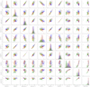 |
Fig. 7 Cross-dependence and distributions of the ten variables considered to be separated according to the branches in Fig. 6. |
4.3 SAX J1808.4−3658
The location of SAX J1808.4−3658 within the MST is also of considerable interest. This source is an accreting millisecond X-ray pulsar (AMXP; see e.g., Patruno & Watts 2021) that has exhibited ten approximately month-long outbursts with a recurrence of about 2–3 years, making it the AMXP with the most numerous outbursts, and suitable for in-depth investigation of its long-term timing properties, as discussed by Illiano et al. (2023). SAX J1808.4−3658 is likely a gamma-ray source (de Oña Wilhelmi et al. 2016), and there is ambiguity regarding its activity status as a rotation-powered millisecond pulsar during quiescent periods, despite the lack of detected radio pulsations Focusing on the long-term first derivative of the spin frequency, as detailed in Fig. 2 and Sect. 3.2 of Illiano et al. (2023), reveals a ![Mathematical equation: $\[\dot{\nu}\]$](/articles/aa/full_html/2024/12/aa50758-24/aa50758-24-eq32.png) = −1.152(56) × 10−15 Hz s−1, in alignment with findings from previous works (Patruno et al. 2012; Sanna et al. 2017; Bult et al. 2020). The variables taken are P = 0.00249391976403(31) s, A1 = 0.0628033(57) lt-s, and PB = 0.083902314(96) d (as listed in Table 1 of Illiano et al. 2023). Consequently, we estimate
= −1.152(56) × 10−15 Hz s−1, in alignment with findings from previous works (Patruno et al. 2012; Sanna et al. 2017; Bult et al. 2020). The variables taken are P = 0.00249391976403(31) s, A1 = 0.0628033(57) lt-s, and PB = 0.083902314(96) d (as listed in Table 1 of Illiano et al. 2023). Consequently, we estimate ![Mathematical equation: $\[\dot{P}\]$](/articles/aa/full_html/2024/12/aa50758-24/aa50758-24-eq33.png) = −
= −![Mathematical equation: $\[\dot{\nu}\]$](/articles/aa/full_html/2024/12/aa50758-24/aa50758-24-eq34.png) /ν2 = −P2
/ν2 = −P2 ![Mathematical equation: $\[\dot{\nu}\]$](/articles/aa/full_html/2024/12/aa50758-24/aa50758-24-eq35.png) ~ 7.2 × 10⁻²¹ s s−1. A previous timing analysis indicates that the neutron star orbits a semi-degenerate companion of MC ~ 0.05 M⊙ (see Bildsten & Chakrabarty 2001). Considering the values computed for the other variables, given the known spin period and spin period derivative, we apply the incremental algorithm to obtain T′. Using the BWs and RBs seen in Fig. 4 as a reference, we show T′ in Fig. 11 together with the AMXP SAX J1808.4−3658, which falls at the gate of the high-density zone of BWs.
~ 7.2 × 10⁻²¹ s s−1. A previous timing analysis indicates that the neutron star orbits a semi-degenerate companion of MC ~ 0.05 M⊙ (see Bildsten & Chakrabarty 2001). Considering the values computed for the other variables, given the known spin period and spin period derivative, we apply the incremental algorithm to obtain T′. Using the BWs and RBs seen in Fig. 4 as a reference, we show T′ in Fig. 11 together with the AMXP SAX J1808.4−3658, which falls at the gate of the high-density zone of BWs.
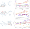 |
Fig. 8 Examples of the values of P, |
![Mathematical equation: $\[\dot{P}\]$](/articles/aa/full_html/2024/12/aa50758-24/aa50758-24-eq36.png)
![Mathematical equation: $\[\dot{E}\]$](/articles/aa/full_html/2024/12/aa50758-24/aa50758-24-eq37.png)
5 Concluding remarks
Graph theory provides an elegant way to inspect a population. The combination of the MST and the underlying distance ranking helps to distinguish the components as well as identify candidates for membership in a particular group. Here we focus on the MSP population and show that its MST forms groups, with BWs and RBs being placed in different regions. This separation is evident when plotting the MC for each system. When the values of MC are not clear-cut between these populations, it is increasingly difficult to make a safe classification without further studies. Based on the locations of our sample of pulsars within the MST, the individual distance ranking for a given pulsar, and the fact that in only very few cases the ranking of a given pulsar thought to pertain to one class is dominated by pulsars belonging to another, we come to the following conclusions:
We promote that J1300+1240, J1630+3550, J1317−0157, J1221−0633, J1627+3219, J1701−3006F, and J1737−0314A be classified as BWs;
The MST location and the ranking favor, or at the very least do not rule out, a BW classification for J1908+2105;
The pulsars J1723−2837, J1902−5105, and J1431−4715 are the only ones in the sample containing at least one known tMSP in their closest three neighbors. We advocate further studies of these pulsars to catch them transitioning into an accretion-powered state in analogy to the known tMSPs;
The MST location of IGR J18245−2452/PSR J1824−2452I, which implies an RB transitional pulsar, suggests that the yet unknown
![Mathematical equation: $\[\dot{P}\]$](/articles/aa/full_html/2024/12/aa50758-24/aa50758-24-eq42.png) is in the range
is in the range ![Mathematical equation: $\[\dot{P}\]$](/articles/aa/full_html/2024/12/aa50758-24/aa50758-24-eq43.png) ~ (1 × 10⁻²⁰, 6 × 10⁻¹⁹) ss−1. Searches limited to this range could empower the techniques and lead to detections;
~ (1 × 10⁻²⁰, 6 × 10⁻¹⁹) ss−1. Searches limited to this range could empower the techniques and lead to detections;Spanning over the uncertainty in the variables of the putative transitional pulsar behind 3FGL J1544.6−1125, we see indeed that it is located near the others in most cases;
The AMXP SAX J1808.4−3658 is close to the group of BWs and can be classified as such from its location in the MST. Indeed, di Salvo et al. (2008) proposed that the system is a hidden BW and that in X-ray quiescence the source is ejecting matter. We note that this fact alone would not necessarily imply its possible BW nature;
If we use graph theory to cluster the population of MSPs via distinguishing branches (unsupervised methodology), we recover a clear distinction between BWs, RBs, and a significant number of other MSPs showing different features, namely larger PB, MC, and P, and smaller
![Mathematical equation: $\[\dot{E}\]$](/articles/aa/full_html/2024/12/aa50758-24/aa50758-24-eq44.png) releases;
releases;This process also separates BWs in the field from those in globular clusters, placing them in different branches within the BW region.
 |
Fig. 9 Minimum spanning tree containing different realizations for |
![Mathematical equation: $\[\dot{P}\]$](/articles/aa/full_html/2024/12/aa50758-24/aa50758-24-eq38.png)
![Mathematical equation: $\[\dot{P}\]$](/articles/aa/full_html/2024/12/aa50758-24/aa50758-24-eq39.png)
![Mathematical equation: $\[\dot{P}\]$](/articles/aa/full_html/2024/12/aa50758-24/aa50758-24-eq40.png)
![Mathematical equation: $\[\dot{P}\]$](/articles/aa/full_html/2024/12/aa50758-24/aa50758-24-eq41.png)
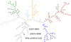 |
Fig. 10 Minimum spanning tree defined as T′(219, 218), containing the 3FGL J1544.6−1125 (in black), with the known tMSPs (in yellow) labeled: J1023+0038 and J1227−4853, as seen in Fig. 4. The color code of the significant branches, trunk, and the remaining pulsars is the same as in Fig. 6. |
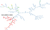 |
Fig. 11 Minimum spanning tree defined as T′(219, 218), containing the AMXP SAX J1808.4−3658 (in black). The confirmed BWs appear in red, RBs in green, tMSPs in yellow, BWs and RBs in globular clusters in light red and light green, the RB candidate in light teal, and the unclassified sources are shown in blue, as seen in Fig. 4. |
Acknowledgements
This work was supported by the grant PID2021-124581OBI00 of MCIU/AEI/10.13039/501100011033 and 2021SGR00426. This work was also supported by the program Unidad de Excelencia María de Maeztu CEX2020-001058-M and by MCIU with funding from the European Union NextGeneration EU (PRTR-C17.I1). CRG is funded by the Ph.D. FPI fellowship PRE2019-090828 acknowledges the graduate program of the Universitat Autònoma of Barcelona. FCZ is supported by a Ramón y Cajal fellowship (grant agreement RYC2021-030888-I). GI, FCZ, AP, and DdM acknowledge financial support from the Italian National Institute for Astrophysics (INAF) Research Grant “Uncovering the optical beat of the fastest magnetized neutron stars” (FANS; PI: AP). GI and AP also acknowledge financial support from the Italian Ministry of University and Research (MUR) under PRIN 2020 grant No. 2020BRP57Z ‘Gravitational and Electromagnetic-wave Sources in the Universe with Current and Next-generation detectors (GEMS)’. GI is supported by the AASS Ph.D. joint research program between the University of Rome “Sapienza” and the University of Rome “Tor Vergata” with the collaboration of the National Institute of Astrophysics (INAF).
Appendix A Variables of BWs, RBs, and tMSPs
Table A.1 shows the values of the variables for BWs, RBs, and tMSPs, both confirmed and candidates, shown in Fig. 4, according to the ATNF catalog.
Variables according to the ATNF catalog of BWs, RBs, and tMSPs.
Appendix B Significant branches
We applied the betweenness centrality estimator (see Freeman 1977; Moxley & Moxley 1974; Brandes 2001; Baron & Ménard 2021) to identify the most central nodes of the graph T. Values seen as outliers in betweenness centrality will be named potential trunk nodes, or pTNs. The trunk is defined as a path, i.e., a sequence of non-repeated nodes. At the end of the trunk, the pTNs that delimit are called contour nodes (CN). These CNs must be nodes of a degree greater than 2, so they act as an articulation point for the graph, i.e., removing these nodes partitions the graph into connected components. The connected components originating in a CN are called contour branches (CB). This leaves a clustered structure with a minimum of two groupings at each extreme of the trunk. To avoid limiting the trunk in nodes of degree 2 or larger but from which the departing structures are of non-representative size (i.e., we aim to avoid noise near the trunk), we define a significant threshold (αs) so that the number of nodes in the CBs is requested to exceed this lower limit. We set the threshold at 5%, i.e. implying that branches will contain at least 11 pulsars of the total population. Once all the possible CNs are identified, we calculate all the possible trunks as the paths that result in pairing these CNs. The number of trunks obtained, therefore, are #Trunks = CNs × (CNs − 1)/2. For each possible trunk, we have a set of branches constituted by the connected components starting from every node of a degree larger than 2 (including the CBs) and having αs as a lower limit to the number of nodes each one must contain.
This results in six sets of branches and trunks. We choose the set that provides greater uniformity in the size of the resulting groups, which contributes to the robustness of a comparison analysis, such as a non-parametric test such as the Kolmogorov-Smirnov (KS) statistics (see e.g., Wolfe 2012; Lehmann 2012; Yadolah 2008). In this case, the null hypothesis (H0) is that the distribution of the variables of the nodes of two given branches is consistent with them coming from the same parent distribution. Rejecting this null hypothesis, say at the 95% confidence level (CL) or better, would lead us to think that two branches may be formed by different pulsars or at different evolution stages. Table B.1 shows the KS test results for these branches, where the H0 column indicates which branches differ the most under the above assumptions. It is observed that most of the branches are distinguished for most of the individual variables.
Comparison of branches via the KS test.
Appendix C No moding in identified tMSP candidates in the radio state
The EPIC-pn (Strüder et al. 2001) operated with a time resolution of 73.4 ms (full frame mode) for 1723-2837 and J1902-5105, and 47.4 ms (large window mode) for J1431-4715. The two EPIC-MOS (Turner et al. 2001) were employed with a time resolution of 2.6 s (full frame mode) in the first two cases and 0.9 s (large window mode) for J1431-4715. We processed and analyzed the data using the Science Analysis Software (SAS; v.21.0.0). All three observations exhibited high background activity in the 10–12 keV light curve, so we excluded the contaminated data intervals. For the EPIC-pn and each MOS, we extracted source photons within a circular region centered on the source position with a 40″radius, and background photons from an 80″wide, source-free circular region. Using the epiclccorr task, 0.3-10 keV background-subtracted light curves were extracted from the three EPIC instruments over the simultaneous coverage time interval, binned with a time resolution of 100 s. As previously noted, we recall that the X-ray flux of J1723-2837 (top panel of Fig. C.1) is variable with the orbital phase as discussed in Bogdanov et al. (2014).
 |
Fig. C.1 XMM-Newton 0.3-10 keV background-subtracted light curves over the time interval in which the three EPIC instruments collected data simultaneously for J1723-2837 (top panel) and J1902-5105 (bottom panel). The light curves are binned with a time resolution of 100 s. For a detailed analysis of J1431-4715 see de Martino et al. (2024); Koljonen & Linares (2023). |
We searched the XMM-Newton light curves for the typical bimodality between ‘high’ and ‘low’ intensity modes (see Fig. C.1; see de Martino et al. (2024), see also, (Koljonen & Linares 2023) for a detailed analysis of J1431-4715). We experimented with different bin sizes but did not observe the expected bimodal feature. Further analysis of the count rate distributions confirmed the absence of this bimodality. A deep search for pulsation has identified PSR J1431-4715 as a gamma-ray pulsar Smith et al. (2023); its gamma-ray emission shows variable signature as those found for prototypical tMSPs Torres et al. (2017).
We note that the prototype for tMSPs, J1023+0038, is located at ~1.37 kpc (Deller et al. 2012), while the estimated distances for J1723-2837 and J1902-5105 are ~0.75 kpc (Bogdanov et al. 2014) and ~1.2 kpc (Camilo et al. 2015), respectively. Assuming comparable luminosities, if a similar bimodal behavior were present, we would expect to observe it in these closer sources.
Moreover, distinct high and low modes are evident in the faint candidate tMSP 3FGL J1544.6-1125 (Bogdanov & Halpern 2015). For the latter source, as a check, we have re-analyzed the XMM-Newton archival observation ObsID 072080101. The bimodal pattern was detected in the EPIC/MOS1 0.3-10 keV background-subtracted light curve binned with a time resolution of 100 s and exhibiting an average count rate comparable to that of J1723-2837. Thus, should it be present in J1723-2837, it should have become similarly apparent.
References
- An, H., Romani, R. W., Kerr, M., & (Fermi-LAT collaboration). 2020, ApJ, 897, 52 [NASA ADS] [CrossRef] [Google Scholar]
- Archibald, A. M., Stairs, I. H., Ransom, S. M., et al. 2009, Science, 324, 1411 [Google Scholar]
- Archibald, A. M., Bogdanov, S., Patruno, A., et al. 2015, ApJ, 807, 62 [NASA ADS] [CrossRef] [Google Scholar]
- Baglio, M. C., Coti Zelati, F., Campana, S., et al. 2023, A&A, 677, A30 [NASA ADS] [CrossRef] [EDP Sciences] [Google Scholar]
- Baron, D., & Ménard, B. 2021, ApJ, 916, 91 [NASA ADS] [CrossRef] [Google Scholar]
- Bassa, C. G., Patruno, A., Hessels, J. W. T., et al. 2014, MNRAS, 441, 1825 [Google Scholar]
- Bates, S. D., Thornton, D., Bailes, M., et al. 2015, MNRAS, 446, 4019 [NASA ADS] [CrossRef] [Google Scholar]
- Bildsten, L., & Chakrabarty, D. 2001, ApJ, 557, 292 [NASA ADS] [CrossRef] [Google Scholar]
- Bogdanov, S., & Halpern, J. P. 2015, ApJ, 803, L27 [NASA ADS] [CrossRef] [Google Scholar]
- Bogdanov, S., Esposito, P., Crawford, Fronefield, I., et al. 2014, ApJ, 781, 6 [Google Scholar]
- Bogdanov, S., Archibald, A. M., Bassa, C., et al. 2015, ApJ, 806, 148 [NASA ADS] [CrossRef] [Google Scholar]
- Braglia, C., Mignani, R. P., Belfiore, A., et al. 2020, MNRAS, 497, 5364 [NASA ADS] [CrossRef] [Google Scholar]
- Brandes, U. 2001, J. Math. Soc., 25, 163 [CrossRef] [Google Scholar]
- Britt, C. T., Strader, J., Chomiuk, L., et al. 2017, ApJ, 849, 21 [NASA ADS] [CrossRef] [Google Scholar]
- Bult, P., Chakrabarty, D., Arzoumanian, Z., et al. 2020, ApJ, 898, 38 [CrossRef] [Google Scholar]
- Camilo, F., Kerr, M., Ray, P. S., et al. 2015, ApJ, 810, 85 [NASA ADS] [CrossRef] [Google Scholar]
- Cassanelli, T., Naletto, G., Codogno, G., et al. 2022, A&A, 663, A106 [NASA ADS] [CrossRef] [EDP Sciences] [Google Scholar]
- Corcoran, K. A., Ransom, S. M., & Lynch, R. S. 2023, RNAAS, 7, 41 [NASA ADS] [Google Scholar]
- Corongiu, A., Mignani, R. P., Seyffert, A. S., et al. 2021, MNRAS, 502, 935 [NASA ADS] [CrossRef] [Google Scholar]
- Coti Zelati, F., Papitto, A., de Martino, D., et al. 2019, A&A, 622, A211 [NASA ADS] [CrossRef] [EDP Sciences] [Google Scholar]
- Crawford, F., Lyne, A. G., Stairs, I. H., et al. 2013, ApJ, 776, 20 [NASA ADS] [CrossRef] [Google Scholar]
- de Amorim, L. B. V., Cavalcanti, G. D. C., & Cruz, R. M. O. 2022, arXiv e-prints [arXiv:2212.12343] [Google Scholar]
- de Martino, D., Belloni, T., Falanga, M., et al. 2013, A&A, 550, A89 [NASA ADS] [CrossRef] [EDP Sciences] [Google Scholar]
- de Martino, D., Phosrisom, A., Dhillon, V. S., et al. 2024, A&A, 691, A36 [NASA ADS] [CrossRef] [EDP Sciences] [Google Scholar]
- Deller, A. T., Archibald, A. M., Brisken, W. F., et al. 2012, ApJ, 756, L25 [NASA ADS] [CrossRef] [Google Scholar]
- Deneva, J. S., Ray, P. S., Camilo, F., et al. 2021, ApJ, 909, 6 [Google Scholar]
- de Oña Wilhelmi, E., Papitto, A., Li, J., et al. 2016, MNRAS, 456, 2647 [CrossRef] [Google Scholar]
- di Salvo, T., Burderi, L., Riggio, A., Papitto, A., & Menna, M. T. 2008, MNRAS, 389, 1851 [NASA ADS] [CrossRef] [Google Scholar]
- Di Salvo, T., Papitto, A., Marino, A., Iaria, R., & Burderi, L. 2023, arXiv e-prints [arXiv:2311.12516] [Google Scholar]
- Douglas, A., Padmanabh, P. V., Ransom, S. M., et al. 2022, ApJ, 927, 126 [NASA ADS] [CrossRef] [Google Scholar]
- Eckert, D., Del Santo, M., Bazzano, A., et al. 2013, The Astronomer’s Telegram, 4925, 1 [Google Scholar]
- Eichler, D., & Levinson, A. 1988, ApJ, 335, L67 [NASA ADS] [CrossRef] [Google Scholar]
- Erickson, J. 2019, Algorithms (Jeff Erickson, Lecture Notes University of Illinois at Urbana-Champaign) [Google Scholar]
- Ferrigno, C., Bozzo, E., Papitto, A., et al. 2014, A&A, 567, A77 [NASA ADS] [CrossRef] [EDP Sciences] [Google Scholar]
- Freeman, L. C. 1977, Sociometry, 40, 35 [Google Scholar]
- Freire, P. C. C., Hessels, J. W. T., Nice, D. J., et al. 2005, ApJ, 621, 959 [NASA ADS] [CrossRef] [Google Scholar]
- Freire, P. C. C., Ridolfi, A., Kramer, M., et al. 2017, MNRAS, 471, 857 [Google Scholar]
- García, C. R. & Torres, D. F. 2023, MNRAS, 520, 599 [CrossRef] [Google Scholar]
- García, C. R., Torres, D. F., & Patruno, A. 2022, MNRAS, 515, 3883 [CrossRef] [Google Scholar]
- Gower, J. C., & Ross, G. J. S. 1969, J. Roy. Statist. Soc. Ser. C (Appl. Statist.), 18, 54 [Google Scholar]
- Hui, C.-Y. 2014, J. Astron. Space Sci., 31, 101 [NASA ADS] [CrossRef] [Google Scholar]
- Illiano, G., Papitto, A., Sanna, A., et al. 2023, ApJ, 942, L40 [NASA ADS] [CrossRef] [Google Scholar]
- Jiang, L., Zhang, C.-M., Tanni, A., & Zhao, H.-H. 2013, in International Journal of Modern Physics Conference Series, 23, 95 [NASA ADS] [CrossRef] [Google Scholar]
- Karttunen, H., Kröger, P., Oja, H., Poutanen, M., & Donner, K. J. 2007, Fundamental Astronomy, 5th edn. (Springer) [CrossRef] [Google Scholar]
- Kennedy, M. R., Breton, R. P., Clark, C. J., et al. 2022, MNRAS, 512, 3001 [NASA ADS] [CrossRef] [Google Scholar]
- Kerr, M., Camilo, F., Johnson, T. J., et al. 2012, ApJ, 748, L2 [NASA ADS] [CrossRef] [Google Scholar]
- King, A. R., Beer, M. E., Rolfe, D. J., Schenker, K., & Skipp, J. M. 2005, MNRAS, 358, 1501 [CrossRef] [Google Scholar]
- Kiziltan, B., & Thorsett, S. E. 2010, ApJ, 715, 335 [Google Scholar]
- Kleinberg, J., & Tardos, E. 2005, Algorithm Design (Addison Wesley) [Google Scholar]
- Koljonen, K. I. I., & Linares, M. 2023, MNRAS, 525, 3963 [NASA ADS] [CrossRef] [Google Scholar]
- Konacki, M., & Wolszczan, A. 2003, ApJ, 591, L147 [NASA ADS] [CrossRef] [Google Scholar]
- Kong, A. K. H., Hui, C. Y., Takata, J., Li, K. L., & Tam, P. H. T. 2017, ApJ, 839, 130 [NASA ADS] [CrossRef] [Google Scholar]
- Kruskal, J. B. 1956, Proc. Amer. Math. Soc., 7, 48 [CrossRef] [Google Scholar]
- Lee, J., Hui, C. Y., Takata, J., et al. 2018, ApJ, 864, 23 [NASA ADS] [CrossRef] [Google Scholar]
- Lehmann, E. L. 2012, in Selected Works of E.L. Lehmann (Springer), 373 [CrossRef] [Google Scholar]
- Lewis, E. F., Olszanski, T. E. E., Deneva, J. S., et al. 2023, ApJ, 956, 132 [NASA ADS] [CrossRef] [Google Scholar]
- Li, M., Halpern, J. P., & Thorstensen, J. R. 2014, ApJ, 795, 115 [NASA ADS] [CrossRef] [Google Scholar]
- Linares, M. 2014, ApJ, 795, 72 [NASA ADS] [CrossRef] [Google Scholar]
- Linares, M., Bahramian, A., Heinke, C., et al. 2014, MNRAS, 438, 251 [NASA ADS] [CrossRef] [Google Scholar]
- Lorimer, D. R., & Kramer, M. 2012, Handbook of Pulsar Astronomy (Cambridge University Press) [Google Scholar]
- Lynch, R. S., Freire, P. C. C., Ransom, S. M., & Jacoby, B. A. 2012, ApJ, 745, 109 [NASA ADS] [CrossRef] [Google Scholar]
- Manchester, R. N. 2017, J. Astrophys. Astron., 38, 42 [NASA ADS] [CrossRef] [Google Scholar]
- Manchester, R. N., Hobbs, G. B., Teoh, A., & Hobbs, M. 2005, AJ, 129, 1993 [Google Scholar]
- Maritz, J., Maritz, E., & Meintjes, P. 2016, The Proceedings of SAIP2016, the 61st Annual Conference of the South African Institute of Physics, eds. S. Peterson, & S. Yacoob (UCT/2016), 243 [Google Scholar]
- Miraval Zanon, A., Burgay, M., Possenti, A., & Ridolfi, A. 2018, in Journal of Physics Conference Series, 956, 012004 [NASA ADS] [CrossRef] [Google Scholar]
- Moxley, R. L., & Moxley, N. F. 1974, Sociometry, 37, 122 [CrossRef] [Google Scholar]
- Pan, Z., Qian, L., Ma, X., et al. 2021, ApJ, 915, L28 [NASA ADS] [CrossRef] [Google Scholar]
- Papitto, A., Ambrosino, F., Stella, L., et al. 2019, ApJ, 882, 104 [NASA ADS] [CrossRef] [Google Scholar]
- Papitto, A. & Bhattacharyya, S. 2022, Millisecond Pulsars (Springer ASSL) [Google Scholar]
- Papitto, A. & de Martino, D. 2022, in Astrophysics and Space Science Library, 465, eds. S. Bhattacharyya, A. Papitto, & D. Bhattacharya, 157 [NASA ADS] [CrossRef] [Google Scholar]
- Papitto, A., Ferrigno, C., Bozzo, E., et al. 2013, Nature, 501, 517 [NASA ADS] [CrossRef] [Google Scholar]
- Patruno, A., & Watts, A. L. 2021, in Astrophysics and Space Science Library, 461, Timing Neutron Stars: Pulsations, Oscillations and Explosions, eds. T. M. Belloni, M. Méndez, & C. Zhang, 143 [NASA ADS] [CrossRef] [Google Scholar]
- Patruno, A., Bult, P., Gopakumar, A., et al. 2012, ApJ, 746, L27 [NASA ADS] [CrossRef] [Google Scholar]
- Patruno, A., Archibald, A. M., Hessels, J. W. T., et al. 2014, ApJ, 781, L3 [Google Scholar]
- Pearson, K. 1901, Lond. Edinb. Dublin Philos. Mag. J. Sci., 2, 559 [CrossRef] [Google Scholar]
- Prim, R. C. 1957, Bell Syst. Tech. J., 36, 1389 [NASA ADS] [CrossRef] [Google Scholar]
- Ray, P. S., Abdo, A. A., Parent, D., et al. 2012, arXiv e-prints [arXiv:1205.3089] [Google Scholar]
- Roberts, M. S. E. 2013, in Neutron Stars and Pulsars: Challenges and Opportunities after 80 years, 291, eds. J. van Leeuwen, 127 [Google Scholar]
- Roberts, M. S. E., Al Noori, H., Torres, R. A., et al. 2018, in Pulsar Astrophysics the Next Fifty Years, 337, eds. P. Weltevrede, B. B. P. Perera, L. L. Preston, & S. Sanidas, 43 [Google Scholar]
- Roughgarden, T. 2019, Algorithms Illuminated (Part 3): Greedy Algorithms and Dynamic Programming (Soundlikeyourself Publishing, LLC) [Google Scholar]
- Sanna, A., Di Salvo, T., Burderi, L., et al. 2017, MNRAS, 471, 463 [NASA ADS] [CrossRef] [Google Scholar]
- Sen, B., Linares, M., Kennedy, M. R., et al. 2024, ApJ, 973, 121 [NASA ADS] [CrossRef] [Google Scholar]
- Shlens, J. 2014, arXiv e-prints [arXiv:1404.1100] [Google Scholar]
- Smith, D. A., Abdollahi, S., Ajello, M., et al. 2023, ApJ, 958, 191 [NASA ADS] [CrossRef] [Google Scholar]
- Sobey, C., Bassa, C. G., O’Sullivan, S. P., et al. 2022, A&A, 661, A87 [NASA ADS] [CrossRef] [EDP Sciences] [Google Scholar]
- Strader, J., Swihart, S., Chomiuk, L., et al. 2019, ApJ, 872, 42 [Google Scholar]
- Strüder, L., Briel, U., Dennerl, K., et al. 2001, A&A, 365, L18 [Google Scholar]
- Swiggum, J. K., Pleunis, Z., Parent, E., et al. 2023, ApJ, 944, 154 [NASA ADS] [CrossRef] [Google Scholar]
- Swihart, S. J., Strader, J., Chomiuk, L., et al. 2022, ApJ, 941, 199 [NASA ADS] [CrossRef] [Google Scholar]
- Tauris, T. M., & van den Heuvel, E. P. J. 2023, Physics of Binary Star Evolution. From Stars to X-ray Binaries and Gravitational Wave Sources [Google Scholar]
- Tauris, T. M., Langer, N., & Kramer, M. 2012, MNRAS, 425, 1601 [NASA ADS] [CrossRef] [Google Scholar]
- Torres, D. F., Ji, L., Li, J., et al. 2017, ApJ, 836, 68 [NASA ADS] [CrossRef] [Google Scholar]
- Turner, M. J. L., Abbey, A., Arnaud, M., et al. 2001, A&A, 365, L27 [CrossRef] [EDP Sciences] [Google Scholar]
- Valiente, G. 2002, Algorithms on Trees and Graphs (Berlin: Springer-Verlag) [CrossRef] [Google Scholar]
- Vleeschower, L., Corongiu, A., Stappers, B. W., et al. 2024, MNRAS, 530, 1436 [NASA ADS] [CrossRef] [Google Scholar]
- Vohl, D., van Leeuwen, J., & Maan, Y. 2024, A&A, 687, A113 [NASA ADS] [CrossRef] [EDP Sciences] [Google Scholar]
- Wilson, R. J. 2010, Introduction to Graph Theory (Pearson) [Google Scholar]
- Wolfe, D. A. 2012, in Selected Works of E.L. Lehmann, ed. J. Rojo (Boston, MA: Springer US), 1101 [CrossRef] [Google Scholar]
- Wolszczan, A. 1994, Science, 264, 538 [NASA ADS] [CrossRef] [Google Scholar]
- Wolszczan, A., & Frail, D. A. 1992, Nature, 355, 145 [CrossRef] [Google Scholar]
- Wolszczan, A., Hoffman, I. M., Konacki, M., Anderson, S. B., & Xilouris, K. M. 2000, ApJ, 540, L41 [NASA ADS] [CrossRef] [Google Scholar]
- Yadolah, D. 2008, in The Concise Encyclopedia of Statistics (New York, NY: Springer New York), 283 [Google Scholar]
- Yan, Z., Shen, Z.-Q., Yuan, J.-P., et al. 2013, MNRAS, 433, 162 [CrossRef] [Google Scholar]
- Yap, Y. X. J., Kong, A. K. H., & Li, K.-L. 2023, ApJ, 955, 21 [NASA ADS] [CrossRef] [Google Scholar]
The notation | · | represents the cardinality (or size) of the specified set, indicating the number of elements within it.
For consistency, we assume ![Mathematical equation: $\[B_{s}=3.2 \times 10^{19} \sqrt{P \dot{P}} \mathrm{G}\]$](/articles/aa/full_html/2024/12/aa50758-24/aa50758-24-eq49.png) .
.
All Tables
All Figures
|
Fig. 1 Distribution of the logarithm of the ten variables considered for the sample of 218 pulsars. |
| In the text | |
|
Fig. 2 Cross-dependence of the ten variables considered. Confirmed BWs (in red) and RBs (in green) are separately noted. For visualization reasons, no distinction is made between MSPs residing in globular clusters and those not, and the tMSPs are marked in green due to their behavior as RBs. The pulsars not yet assigned to any of these classes are shown in blue. The main diagonal shows the distribution for each variable. The panels with the shaded background show the pairs formed with PB, MC, and A1, which best differentiate the BWs from the rest. |
| In the text | |
|
Fig. 3 PCA results for the logarithm of the set of variables for the whole population of 218 MSPs. The left panel, also called the scree plot, shows the explained variance of each PC according to the eigenvalues of the covariance matrix. We note that the covariance matrix calculates the relationships between pairs of variables, showing how changes in one variable are associated with changes in another. It represents the amount of information contained in each PC. The central panel shows the cumulative explained variance by the new variables defined through the PCA analysis. The right panel shows the “weight” (also called loading) that each variable has concerning each PC, indicating its contribution to the variance captured by that PC. This value is the coefficient held in each eigenvector of the covariance matrix. Negative values imply that the variable and the PC are negatively correlated. Conversely, a positive value shows a positive correlation between the PC and the variable. |
| In the text | |
|
Fig. 4 Minimum spanning tree of the binary pulsar population defined as T(218, 217) based on the complete, undirected, and weighted graph G(218, 23 653) computed from the Euclidean distance among ten scaled variables (or the equivalent four PCs that describe their whole variance). Each node in the MST represents a pulsar. The MST separately notes confirmed BWs (red), RBs (green), and tMSPs J1023+0038 and J1227−4853 (yellow), respectively. Also, the BWs and RBs in globular clusters (light red and light green, respectively) are highlighted. The RBs J1622−0315 (green) and the RB candidate J1302−3258 (light teal) are also noted in the rightmost branch of the MST. The unclassified ones appear in blue. See Table A.1 for more details. |
| In the text | |
|
Fig. 5 Zoom onto the leftmost part of the MST shown in Fig. 4. The locations of the pulsars (shown in orange) discussed in Sect. 2.3.1 (left panel), Sect. 2.3.2 (central panel), and Sect. 2.3.3 (right panel) can be seen more clearly here. The same color code is used as in Fig. 4, where the confirmed BWs appear in red, RBs in green, tMSPs in yellow, and the BWs and RBs in globular clusters are shown in light red and light green, keeping the unclassified pulsars in blue. |
| In the text | |
|
Fig. 6 Minimum spanning tree of the MSP population is defined as T(218, 217), separated into significant branches according to the algorithm described in the text (see Sect. 3). The branches group a comparable number of pulsars: gray (39), orange (20), dark blue (31), brown (54), dark green (30), and pink (16). The trunk (in dark khaki) has only 14 nodes, with 14 others (in sky blue) that are not considered to pertain to any significant branch or trunk and appear to be the noise of the former structures. |
| In the text | |
|
Fig. 7 Cross-dependence and distributions of the ten variables considered to be separated according to the branches in Fig. 6. |
| In the text | |
|
Fig. 8 Examples of the values of P, |
| In the text | |
|
Fig. 9 Minimum spanning tree containing different realizations for |
| In the text | |
|
Fig. 10 Minimum spanning tree defined as T′(219, 218), containing the 3FGL J1544.6−1125 (in black), with the known tMSPs (in yellow) labeled: J1023+0038 and J1227−4853, as seen in Fig. 4. The color code of the significant branches, trunk, and the remaining pulsars is the same as in Fig. 6. |
| In the text | |
|
Fig. 11 Minimum spanning tree defined as T′(219, 218), containing the AMXP SAX J1808.4−3658 (in black). The confirmed BWs appear in red, RBs in green, tMSPs in yellow, BWs and RBs in globular clusters in light red and light green, the RB candidate in light teal, and the unclassified sources are shown in blue, as seen in Fig. 4. |
| In the text | |
|
Fig. C.1 XMM-Newton 0.3-10 keV background-subtracted light curves over the time interval in which the three EPIC instruments collected data simultaneously for J1723-2837 (top panel) and J1902-5105 (bottom panel). The light curves are binned with a time resolution of 100 s. For a detailed analysis of J1431-4715 see de Martino et al. (2024); Koljonen & Linares (2023). |
| In the text | |
Current usage metrics show cumulative count of Article Views (full-text article views including HTML views, PDF and ePub downloads, according to the available data) and Abstracts Views on Vision4Press platform.
Data correspond to usage on the plateform after 2015. The current usage metrics is available 48-96 hours after online publication and is updated daily on week days.
Initial download of the metrics may take a while.