| Issue |
A&A
Volume 691, November 2024
|
|
|---|---|---|
| Article Number | A226 | |
| Number of page(s) | 16 | |
| Section | Galactic structure, stellar clusters and populations | |
| DOI | https://doi.org/10.1051/0004-6361/202451377 | |
| Published online | 15 November 2024 | |
A comparative high-resolution spectroscopic analysis of in situ and accreted globular clusters
1
INAF – Astrophysics and Space Science Observatory of Bologna,
Via Gobetti 93/3,
40129
Bologna,
Italy
2
Department of Physics and Astronomy, University of Bologna,
Via Gobetti 93/2,
40129
Bologna,
Italy
3
Astronomisches Rechen-Institut, Zentrum für Astronomie der Universität Heidelberg,
Mönchhofstraße 12–14,
69120
Heidelberg,
Germany
4
Kapteyn Astronomical Institute, University of Groningen,
Landleven 12,
9747 AD
Groningen,
The Netherlands
★ Corresponding author; This email address is being protected from spambots. You need JavaScript enabled to view it.
Received:
4
July
2024
Accepted:
7
October
2024
Abstract
Globular clusters (GCs) are extremely intriguing systems that help in reconstructing the assembly of the Milky Way via the characterisation of their chemo-chrono-dynamical properties. In this study, we use high-resolution spectroscopic archival data from UVES and UVES-FLAMES at the VLT to compare the chemistry of GCs dynamically tagged as either Galactic (NGC 6218, NGC 6522, and NGC 6626) or accreted from distinct merger events (NGC 362 and NGC 1261 from Gaia-Sausage-Enceladus, and Ruprecht 106 from the Helmi Streams) in the metallicity regime where abundance patterns of field stars with different origin effectively separate (−1.3 ≤ [Fe/H] ≤ −1.0 dex). We find remarkable similarities in the abundances of the two Gaia-Sausage-Enceladus GCs across all chemical elements. They both display depletion in the α-elements (Mg, Si and Ca) and statistically significant differences in Zn and Eu compared to in situ GCs. Additionally, we confirm that Ruprecht 106 exhibits a completely different chemical makeup from the other target clusters, being underabundant in all chemical elements. This demonstrates that when high precision is achieved, the abundances of certain chemical elements can not only efficiently separate in situ from accreted GCs, but can also distinguish among GCs born in different progenitor galaxies. In the end, we investigate the possible origin of the chemical peculiarity of Ruprecht 106. Given that its abundances do not match the chemical patterns of the field stars associated with its most likely parent galaxy (i.e. the Helmi Streams), being depleted in the abundances of α-elements in particular, we believe Ruprecht 106 to originate from a less massive galaxy compared to the progenitor of the Helmi Streams.
Key words: stars: abundances / Galaxy: formation / globular clusters: general
© The Authors 2024
 Open Access article, published by EDP Sciences, under the terms of the Creative Commons Attribution License (https://creativecommons.org/licenses/by/4.0), which permits unrestricted use, distribution, and reproduction in any medium, provided the original work is properly cited.
This article is published in open access under the Subscribe to Open model. This email address is being protected from spambots. You need JavaScript enabled to view it. to support open access publication.
1 Introduction
The latest data releases of the ESA/Gaia mission (Gaia Collaboration 2021, 2023) have instigated a profound transformation of our comprehension of the early chronicles of the Milky Way (MW). This enormous 6D phase space dataset has led to a clearer understanding of the roles played by various mergers in shaping the Galactic halo (see Helmi 2020 for a review), as predicted by simulations in the ACDM cosmological framework (White & Frenk 1991; Moore et al. 1999; Helmi & de Zeeuw 2000; Newton et al. 2018). The imprint of accretion events manifests dynamically as stellar streams (Helmi et al. 1999; Ibata et al. 2024), substructures discernible in phase space (e.g. Helmi et al. 2018; Belokurov et al. 2018; Myeong et al. 2018; Koppelman et al. 2019), and dwarf galaxies whose disruption is currently ongoing (Ibata et al. 1994; Majewski et al. 2003). During such events, not only field stars but also globular clusters (GCs) can survive the merging processes, contributing to the formation of the present-day MW GC system (Brodie & Strader 2006; Peñarrubia et al. 2009; Bellazzini et al. 2020; Trujillo-Gomez et al. 2021). Leveraging the extremely precise kinematic data provided by the Gaia mission, the orbits of MW GCs have been reconstructed with exceptional precision. Through the analysis of their orbital properties, MW GCs have been classified into distinct groups by several authors (Massari et al. 2019; Forbes 2020; Callingham et al. 2022; Chen & Gnedin 2024), distinguishing those accreted from disrupted dwarf galaxies, such as Gaia-Sausage-Enceladus (GSE, Belokurov et al. 2018; Helmi et al. 2018), Sequoia (Myeong et al. 2018), and the Helmi Streams (Helmi et al. 1999), from those formed in situ. Complications may arise in the interpretation of these findings due to the complex and overlapping distribution of GCs in the spaces defined by their orbital parameters (Callingham et al. 2022). This complexity is further exacerbated when accounting for the impact of a non-static potential in the computation of a GC orbit (Amarante et al. 2022; Belokurov et al. 2023; Pagnini et al. 2023; Chen & Gnedin 2024). Nonetheless, it has been established that dynamically tagged groups of GCs lay on different sequences in the age-metallicity space (Kruijssen et al. 2019; Massari et al. 2019; Myeong et al. 2019), confirming the dual nature of the MW GC system in this plane already found in the pre-Gaia era (Marín-Franch et al. 2009; Forbes & Bridges 2010; Leaman et al. 2013; VandenBerg et al. 2013). In particular, it has been demonstrated that older systems at fixed metallicity are more likely to be born in galaxies with a higher star formation efficiency – such as the MW in its earliest phases – compared to dwarf galaxies (e.g. Massari et al. 2023).
This intricate perspective of the assembly history of the MW can be further enriched by the addition of chemical abundance data obtained either from high-resolution spectra or large spec-troscopic surveys (Venn et al. 2004; Nissen & Schuster 2010; Helmi et al. 2018; Horta et al. 2020; Minelli et al. 2021; Limberg et al. 2022; Malhan et al. 2022; Naidu et al. 2022a; Horta et al. 2023; Monty et al. 2023a; Ceccarelli et al. 2024). However, when looking at the distribution of GCs in chemical spaces, the differences between these two populations are subtle, complicating the task of interpreting the results. For instance, Recio-Blanco (2018) highlights a very low scatter in the [α/Fe] ratio among GCs with [Fe/H] <−0.8 dex regardless of their origin. On a similar note, Horta et al. (2020) employed the [Si/Fe] ratio from APOGEE DR17 (Abdurro’uf et al. 2022) of 46 GCs to explore whether their distribution in chemical spaces reflects the kinematically defined classification by Massari et al. (2019). Interestingly, Horta et al. (2020) observed that the positions of both in situ and accreted subgroups in this chemical space align with those of their field-star counterparts. However, they were unable to effectively identify different behaviours from GCs that were brought in by separate progenitors, possibly because of the higher precision needed. Recently, Belokurov & Kravtsov (2024) discriminated between Galactic and extragalactic origin for MW GCs using the [Al/Fe] ratios, building upon the findings of Belokurov & Kravtsov (2022). However, caution should be exercised when using the abundances of light elements in GCs owing to the impact of multiple populations (Bastian & Lardo 2018). Finally, Monty et al. (2023a,b) showcased the efficacy of differential chemical analysis on GCs. Their works not only revealed chemical inhomogeneity at a precision level of 0.02 dex for all chemical elements in GCs, but also showed distinctions in the chemical compositions of two GCs, NGC 288 and NGC 362, associated with the same progenitor, GSE. Specifically, NGC 288 and NGC 362 exhibit dissimilarities in their chemical makeup, particularly in their neutron-capture elements. This difference could be interpreted either as stemming from chemical inhomogeneities in the progenitor or as a consequence of internal chemical evolution within the GCs. In light of all the mentioned complexities, which underline the challenges associated with interpreting results when comparing diverse studies, it becomes evident that maintaining homogeneity is imperative in conducting chemical analyses aimed at verifying the origin of GCs.
In the present study, we derived fully homogeneous detailed elemental abundances of several species for six GCs with similar metallicity (−1.3 ≤ [Fe/H] ≤−1.0 dex) that have been consistently associated with different progenitors (see below) according to all post-Ga/a investigations (Massari et al. 2019; Forbes 2020; Callingham et al. 2022; Chen & Gnedin 2024). These GCs lie in the metallicity range best suited to chemical tagging studies, where abundance trends of in situ and accreted objects start to significantly part ways (Nissen & Schuster 2010; Helmi et al. 2018; Matsuno et al. 2022b). Three of the target clusters, namely NGC 362, NGC 1261, and Ruprecht 106 (Rup106 hereafter), lie on the younger branch of the Galactic GC age-metallicity relation (AMR, Dotter et al. 2010; Dotter et al. 2011), which is interpreted as suggesting an accreted origin. Specifically, due to the characteristics of the spaces defined by the integrals of motion, they have been assigned to GSE (NGC 362 and NGC 1261) and the Helmi Streams (Rup106). Also, we selected three targets (NGC 6218, NGC 6522, and NGC 6626) that are generally considered to have formed in situ, as they fit the older branch of the AMR (Dotter et al. 2010; Dotter et al. 2011; Villanova et al. 2017; Kerber et al. 2018) and move on orbits compatible with either the MW disc (NGC 6218) or the MW bulge (NGC 6522 and NGC 6626). The primary objective of the present work is to test precise chemical tagging as a tool to infer the origin of GCs. When complementing chrono-dynamical information, it is possible to use chemical tagging to clarify the differences among clusters with ambiguous associations. Furthermore, this approach enables determination of whether or not the progenitor galaxy and the associated GC candidates are chemically compatible. For this to be effective, we require a combination of high precision in abundance derivations, which can only be achieved using high-quality data, and homogeneity in the detailed analysis. This is why we reanalysed these six clusters, allowing us to compare them with each other with the utmost precision.
The paper is structured as follows. In Sect. 2 we list the observations that were collected to compile the spectroscopic dataset. In Sect. 3 we describe the methodology employed to carry out the chemical analysis. In Sect. 4 we show the output of the analysis. In Sect. 5 we compare our results with the literature. In Sect. 6 we discuss the peculiarity of Ruprecht 106. In Sect. 7 we summarise the main results of this work.
2 Observations
We retrieved our entire spectroscopic dataset from the ESO archive. The spectra of these stars were all acquired using the multi-object spectrograph UVES-FLAMES (Pasquini et al. 2002) or UVES (Dekker et al. 2000) mounted at the Very Large Telescope (VLT) of the European Southern Observatory. Stars were observed using the Red Arm 580 CD3 grating with a spectral coverage between 4800 and 6800 Å and a spectral resolution of R=40 000. Typical signal-to-noise ratios for these spectra are in the range of 40 ≤ S/N ≤ 65 at 5000 Å and 60 ≤ S/N ≤ 90 at 6000 Å. The spectra were reduced using the dedicated ESO pipeline1, which includes bias subtraction, flat-fielding, wavelength calibration, spectral extraction, and order merging. For the stars observed with UVES at the VLT, the contribution of the sky was properly removed from each stellar spectrum during the pipeline reduction. For the stars observed with UVES-FLAMES at the VLT, the sky contribution was taken into account by acquiring the spectra of some nearby sky regions at the same time as the science targets and subtracting it from each individual exposure. In the end, single exposures of the same star were merged to obtain the final spectrum for each target. Figure 1 shows the spectra of six stars, one per target cluster, to showcase the quality of the dataset.
As mentioned in Sect. 1, the sample of GCs studied here was selected based on their similar metallicity and dynamical association (which is consistent among the different studies; e.g. Massari et al. 2019; Forbes 2020; Callingham et al. 2022, see below). The individual spectroscopic targets analysed in this work were selected as follows:
NGC 362. This cluster has been categorised as accreted during the merger with GSE. The mean metallicity of NGC 362 is [Fe/H] = −1.17 ± 0.05 dex (Carretta et al. 2013). We collected the spectra of 14 RGB stars observed under the ESO-VLT Programme 083.D-0208 (PI: E. Carretta).
NGC 1261. This GC has also been associated with the GSE accretion event. The mean metallicity of this cluster is [Fe/H] = −1.28 ± 0.02 dex (Marino et al. 2021). Our dataset includes the spectra of 12 RGB stars. Among them, 6 were observed under the ESO-VLT Programme 0101.D-0109 (PI: A. Marino), 4 under the ESO-VLT Programme 197.B-1074 (PI: G. F. Gilmore), and 2 under the ESO-VLT Programme 193.D-0232 (PI: F. R. Ferraro).
NGC 6218. This system is an in situ GC located in the MW disc. NGC 6218 has a mean metallicity of [Fe/H] = −1.33 ± 0.08 dex (Carretta et al. 2009). We include in our analysis 11 RGB stars observed under the ESO-VLT Programme 073.D-0211 (PI: E. Carretta).
NGC 6522. This ia an in situ cluster placed in the MW bulge. Its mean metallicity is [Fe/H] = –1.16 ± 0.05 dex (Barbuy et al. 2021). Our sample is composed of four RGB stars observed under the ESO-VLT Programme 097.D-0175 (PI: B. Barbuy).
NGC 6626. This is also an in situ MW bulge GC with a mean metallicity of [Fe/H] = −1.29 ± 0.01 dex (Villanova et al. 2017). We collected the spectra of 16 RGB stars observed under the ESO-VLT Programme 091.D-0535 (PI: C. Moni Bidin).
Ruprecht 106. Among the population of accreted GCs, one that has always attracted significant attention within the community is Rup106. Its orbit is typical of the Galactic halo (Frelijj et al. 2021) and due to its positioning in the spaces defined by the integrals of motion, this GC has been tentatively linked with the progenitor of the Helmi Streams. The chemical peculiarity of Rup106 has been revealed by several spectroscopic analyses (e.g. Brown et al. 1997; Villanova et al. 2013, V13 hereafter), which find that all Rup106 target spectra are depleted in [α/Fe] compared to GCs and field stars of the same metallicity, that is [Fe/H] = −1.37 ± 0.11 dex (Lucertini et al. 2023). We collected the spectra of nine RGB stars that have been observed under the ESO-VLT Programme 069.D-0642 (PI: P. François).
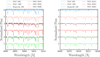 |
Fig. 1 Spectra of stars from the six target clusters observed with UVES and UVES-FLAMES at the VLT at different wavelengths. The spectra have been vertically shifted for the sake of clarity. |
3 Chemical analysis
3.1 Stellar parameters
We derived both the effective temperature (Teff) and the surface gravity (log g) exploiting the Gaia Data Release 3 (DR3, Gaia Collaboration 2023) photometric dataset. It is important to note that stars in GCs are located at significant distances and within crowded environments, which may result in a slight degradation of the quality of Gaia photometry. Stars with ruwe > 1.4 were flagged because their photometry might be of lower quality (Gaia Collaboration 2021).
We determined the Teff for all the targets of our sample using the empirically calibrated (BP – RP)0–Teff relation provided by Mucciarelli et al. (2021a). The choice of using the (BP – RP) colour is guided by the fact that it is the most extended in wavelength among Gaia colours, thus ensuring an optimal sampling of the spectral energy distribution. This approach also eliminates the need to rely on measurements from other photometric systems, which may have lower precision than Gaia. We verified that using other Gaia colours results in Teff differences that are consistently smaller than 50 K, which is below the current uncertainties. The colour excess E(B–V) adopted for each GC is taken from Harris (2010). Given the high extinction in the direction of the Galactic bulge, we corrected the Gaia photometry of NGC 6522 and NGC 6626 for effects of differential reddening following the prescription described in Milone et al. (2012), and using the Cardelli et al. (1989) extinction law. This analysis was performed on the catalogues provided by Vasiliev & Baumgardt (2021), focusing on stars with a probability membership of >90%. The effects of the extinction on the observed colour (BP – RP) have been taken into account following the iterative prescription described in Gaia Collaboration (2018). As the colour–Teff relation we employed is sensitive to the metallicity of the star, we assumed the [Fe/H] value listed in the Harris (2010) catalogue as representative of the GC under investigation to get an initial estimate of Teff. We note that estimating the Teff using the derived [Fe/H] values leads to differences from the initial values consistently lower than 20 K. Internal errors in Teff due to the uncertainties in photometric data, reddening, and the assumed colour–Teff relation are in the range of 80–110 K. We estimated surface gravities from the Stefan-Boltzmann relation using the photometric Teff and a representative stellar mass of 0.8 M⊙, typical for RGB stars in old isochrones at this metallicity, the G-band bolometric corrections described by Andrae et al. (2018), and the distance provided by Baumgardt & Vasiliev (2021). The uncertainties on the log g were derived through the propagation of the errors on Teff, photometry, and distance, and they are always under 0.1 dex. In the end, we calculated microturbulent velocities (υt) by minimising the trend between iron abundances and reduced equivalent widths, defined as log10(EW/λ). To do so, we used ≥100 iron lines per star on average. We assumed a conservative uncertainty of 0.2 km s−1. All the atmospheric parameters are listed in Table 1.
Selected target information (extract).
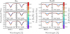 |
Fig. 2 Comparison around the 4810.5 Å Zn (left panel) and the 6645.1 Å EuII (right panel) lines between the observed spectra and seven synthetic spectra computed assuming the derived atmospheric parameters for each star and varying the level of [Zn/Fe] and [EuII/Fe]. The variations are computed with respect to the abundances measured in Rup106. |
3.2 Deriving the abundances
The determination of chemical abundances of Mg, Si, Ca, TiI, TiII, Cr, Fe, Ni, and Zn was conducted by means of a comparative analysis between the observed equivalent widths (EWs) – measured with the code DAOSPEC (Stetson & Pancino 2008) and using the automatic tool 4DAO (Mucciarelli 2013) – and theoretical line strengths. This analysis was executed using the code GALA (Mucciarelli et al. 2013).
We employed the spectral synthesis using the proprietary code SALVADOR to derive the chemical abundances for the species that have hyperfine or isotopic splitting transitions (ScII, V, Mn, Co, Cu, YII, BaII, LaII, and EuII). SALVADOR runs a χ2 -minimisation between the observed line and a grid of suitable synthetic spectra computed on the fly by the code SYNTHE (Kurucz 2005) varying only the abundance of the matching element and keeping the stellar parameters fixed. Synthetic spectra were computed using all the atomic and molecular transitions available in the Kurucz/Castelli2 database.
We used ATLAS9 (Kurucz 2005) model atmospheres computed assuming plane-parallel geometry, hydrostatic and radiative equilibrium, and local thermodynamic equilibrium for all the chemical elements. We started from an α-enhanced model atmosphere ([α/Fe] = +0.4 dex) for all the target GCs except for Rup106, for which we used a solar-scaled chemical mixture according to the values of [α/Fe] we derived. Examples of fits around absorption lines of elements of interest (i.e. Zn and EuII; see Sects. 4.2 and 4.3) are displayed in Fig. 2. Different synthetic spectra are computed for each star by assuming the atmospheric parameters derived as described in Sect. 3.1, and varying the abundances of Zn and EuII. Finally, we scale the abundance ratios to the solar values using the chemical composition described in Grevesse & Sauval (1998), as ATLAS9 model atmospheres are computed based on this solar mixture (Castelli & Kurucz 2003).
3.3 Abundance uncertainties
During the determination of the uncertainties associated with abundance ratios, it is imperative to account for two principal sources of error: first, internal errors stemming from the measurement of the EW, and second, errors originating from the selection of atmospheric parameters.
We estimated the uncertainties attributed to EW measurements as the dispersion observed around the mean of individual line measurements divided by the root mean square of the number of lines employed in the analysis.
The internal error on chemical abundances derived with spectral synthesis were quantified using Monte Carlo simulations. To do so, we repeated the analysis on 1000 noisy synthetic spectra obtained adding Poissonian noise in order to mimic the S/N of the real spectra. The uncertainty is estimated as the standard deviation of the abundance distribution of the 1000 noisy synthetic spectra.
Finally, we performed new calculations of the chemical abundances, considering also the uncertainties associated with the atmospheric parameters. This involved varying one stellar parameter at a time while keeping the others fixed. In the end, all the sources of error are added in quadrature. Given that our chemical abundances are expressed as abundance ratios ([X/Fe]), the uncertainties on the iron abundance [Fe/H] have been taken into account. We estimated the total uncertainty as the squared sum of these two components. Therefore, the final errors were calculated as:
![Mathematical equation: ${\sigma _{[{\rm{Fe}}/{\rm{H}}]}} = \sqrt {{{\sigma _{Fe}^2} \over {{N_{Fe}}}} + {{\left( {\delta _{Fe}^{{T_{{\rm{eff }}}}}} \right)}^2} + {{\left( {\delta _{Fe}^{\log g}} \right)}^2} + {{\left( {\delta _{Fe}^{{{\rm{\v }}_{\rm{t}}}}} \right)}^2}} ,$](/articles/aa/full_html/2024/11/aa51377-24/aa51377-24-eq1.png) (1)
(1)
![Mathematical equation: $\eqalign{ & {\sigma _{[X/Fe]}} = \cr & \sqrt {{{\sigma _X^2} \over {{N_X}}} + {{\sigma _{Fe}^2} \over {{N_{Fe}}}} + {{\left( {\delta _X^{{T_{{\rm{eff }}}}} - \delta _{Fe}^{{T_{{\rm{eff }}}}}} \right)}^2} + {{\left( {\delta _X^{\log g} - \delta _{Fe}^{\log g}} \right)}^2} + {{\left( {\delta _X^{{{\rm{\v }}_{\rm{t}}}} - \delta _{Fe}^{{{\rm{\v }}_{\rm{t}}}}} \right)}^2}} , \cr} $](/articles/aa/full_html/2024/11/aa51377-24/aa51377-24-eq2.png) (2)
(2)
where σX,Fe is the dispersion around the mean of chemical abundances, NX,Fe is the number of used lines, and  are the abundance differences obtained by varying the parameter i.
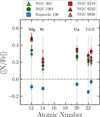 |
Fig. 3 Comparison of mean abundance ratios of the α-elements [Mg/Fe], [Si/Fe], [Ca/Fe], [Til/Fe], and [Till/Fe] for target GCs NGC 362 (green triangles), NGC 1261 (dark green circles), NGC 6218 (red squares), NGC 6522 (brown trianges), NGC 6626 (pink triangles), and Rup106 (blue squares). Error bars indicate the standard deviation. |
4 Abundances of target GCs
In this section, we discuss the abundances of α-, iron-peak, and neutron-capture elements of our target GCs. We exercise caution when interpreting the abundances of certain chemical elements that may be influenced by the presence of multiple populations within GCs (e.g. O, Na, Mg, and Al; see Bastian & Lardo 2018). Among these species, we focus on Mg, which exhibits minimal dispersion within five out of the six GCs in our sample. This outcome aligns with expectations, particularly considering that most of the targeted systems belong to the low-mass and high-metallicity regime of the MW GC system, where the efficiency of the MgAl burning channel diminishes (Ventura et al. 2013; Dell’Agli et al. 2018; Alvarez Garay et al. 2024). Indeed, we find spread in the distribution of [Mg/Fe] only in the most massive among our target cluster, NGC 6626. As we are only concerned with the pristine chemical composition of the gas that formed the cluster, we derived the mean value of [Mg/Fe] using only firstgeneration stars. The results obtained from the homogeneous chemical analysis of 66 RGB stars of the sample of six GCs are listed in Tables 2–4. The mean abundances for each GC are available in Table 5. The average abundance ratios of the target GCs are illustrated in Figs. 3–5.
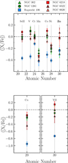 |
Fig. 4 Comparison of mean abundance ratios of the iron-peak elements [ScII/Fe], [V/Fe], [Cr/Fe], [Mn/Fe], [Co/Fe], [Ni/Fe], and [Zn/Fe] for target GCs (top panel). In the bottom panel we plot the two elements ([Cu/Fe] and [YII/Fe]) with the largest differences observed for Rup106. The colour coding is the same as in Fig. 3. Error bars indicate the standard deviation. |
4.1 α-elements
Figure 3 shows the mean values of the α-elements abundances. These chemical elements are predominantly synthesised in massive stars and subsequently dispersed into the interstellar medium through core-collapse supernovae (CC-SNe, Kobayashi & Nomoto 2009; Romano et al. 2010; Kobayashi et al. 2020) events. Additionally, there is a minor but discernible contribution from Type Ia supernovae (SNe Ia), which is particularly notable for Ca and Ti, as discussed in Kobayashi et al. (2020).
First of all, we find that the two GCs associated to GSE (green filled symbols) show identical abundances, within the uncertainties, in all the analysed α-elements. Second, we show that the mean abundances of Mg, Si, and Ca of the three in situ GCs, namely NGC 6218, NGC 6522, and NGC 6626 (red, brown and pink filled symbols, respectively), are fully compatible among each other. For Ti, this consistency is less evident. Third, we find that NGC 362 and NGC 1261 are α-depleted compared to the in situ GCs. They display differences in the α-element at the 1σ level in Mg and Ca when comparing the average abundances and the respective standard deviations (see Appendix A.1 for a comparison with literature). Finally, we derive subsolar abundances in the α-elements of Rup106 (blue filled squares), specifically with [α/Fe] ~ − 0.1 dex, which is in good agreement with the literature (Brown et al. 1997, V13; see Appendix A.2 for a comparison with the results of V13). This is, on average, 0.3–0.4 dex lower than the other five target clusters.
These results guide us as to the degree to which we can use α-elements to distinguish the origin of GCs. The observed trend is a good match to our expectations based on the cluster chrono-dynamical associations. Indeed, GSE clusters NGC 1261 and NGC 362 share the same α-element abundances, as expected for clusters accreted from the same progenitor, with lower [α/Fe] values compared to NGC 6218, NGC 6522, and NGC 6626. Indeed, the in situ GCs consistently show higher [α/Fe] abundances, as predicted for systems born in the MW at this metallicity, where the contribution of SNIa to the gas chemical enrichment was not yet significant. Finally, Rup106 has an even lower [α/Fe] than the GSE GCs, and can be distinguished from them in this respect; this indicates an even more different birth environment, probably characterised by very low star formation efficiency.
Chemical abundances for the α-elements for the target stars (extract).
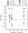 |
Fig. 5 Comparison of mean abundance ratios of the neutron-capture elements [BaII/Fe], [LaII/Fe], and [EuII/Fe] for our target GCs. The colour coding is the same as in Fig. 3. Error bars indicate the standard deviation. |
4.2 Iron-peak elements
Iron-peak elements primarily originate in Type II CC-SNe and hypernovae (HNe), with some contribution also from SNe Ia. Specifically, elements such as Sc, Cu, and Zn are predominantly synthesised by massive stars, while for V and Co the contribution of SNe Ia is not negligible. On the other hand, Cr, Mn, and Ni are primarily produced by SNe Ia (Romano et al. 2010; Kobayashi et al. 2020).
The results shown in Fig. 4 indicate that most of the iron-peak elements do not provide a means to effectively and clearly discriminate between in situ and GSE clusters. Indeed, our target GCs display coherent values in all the chemical spaces with the exception, once again, of Rup106, which is underabundant in ScII, V, Mn, Co, and Ni. In the bottom panel of Fig. 4, we highlight the two elements where Rup106 is most depleted compared to the other systems. Specifically, Cu is the most under-abundant among the chemical elements derived in this work ([Cu/Fe] = −0.95 dex for Rup106). Such low values of [Cu/Fe] can be reproduced in stellar systems with a chemical evolutionary model assuming very inefficient star formation (star formation rate <5 × 10⁻⁴ M⊙ yr−1, Mucciarelli et al. 2021b). Thus, the pronounced depletion in all of these elements might indicate that Rup106 was born in an environment where the contribution of massive stars was extremely low.
Among the iron-peak elements, the only one to demonstrate a statistically significant difference between accreted and in situ GCs is Zn: all the in situ GCs are overabundant with respect to GSE GCs and Rup106 at the 1σ level. In passing, we note that NGC 6626 shows a significant spread in [Zn/Fe], as already found in Villanova et al. (2017). Zn therefore appears to be a good tracer of the in situ or accreted origin of GCs, but it is not sensitive enough to help distinguish among different accreted progenitors. Such a conclusion was also drawn by Minelli et al. (2021), even though these authors used a sample of GCs at higher metallicity. Indeed, high [Zn/Fe] ratios are expected for in situ GCs, and the rationale behind this expectation lies in the fact that the primary contributors to Zn production are hypernovae, which are linked to stars with masses of around 25–30 M⊙ (Romano et al. 2010; Kobayashi et al. 2020). Consequently, galaxies with lower star formation rates should manifest lower [Zn/Fe] ratios due to the reduced impact of massive stars (Yan et al. 2020).
Chemical abundances for the iron-peak elements for the target stars (extract).
Chemical abundances for the neutron-capture elements for the target stars (extract).
4.3 Neutron-capture elements
Slow (s-) neutron-capture elements are mainly synthesised in asymptotic giant branch (AGB) stars. In particular, light s-process elements (e.g. Y) are produced to a large extent by intermediate-mass AGB stars. Conversely, heavy s-process elements (e.g. Ba, La) are mainly produced in AGB stars with masses lower than 4 M⊙ (Kobayashi et al. 2020). Rapid (r-) neutron-capture elements (e.g. Eu) are synthesised during a broad spectrum of events, such as special types of CC-SNe (rCCSNe, e.g. magnetorotational SNe, collapsars; Mösta et al. 2018; Siegel et al. 2019; Kobayashi et al. 2020) and neutron-star mergers (NSMs, Lattimer & Schramm 1974).
First of all, we observe that the in situ NGC 6218 is enhanced (≥0.2 dex) in [YII/Fe] compared to the other two in situ GCs and two GSE GCs. Additionally, among the neutron-capture elements, this is the chemical space in which Rup106 is the most depleted (see the bottom panel of Fig. 4). This finding is particularly intriguing, as Cu, the other element where Rup106 is notably depleted, is also produced by massive stars through weak s-processes, with a small contribution also by AGB stars (Kobayashi & Nomoto 2009; Kobayashi et al. 2020). Thus, if the lack of weak s-process products is responsible for the low derived Cu abundance, light neutron-capture elements are also expected to be similarly depleted, as is observed for Y.
When examining the abundances of the other neutron-capture elements (see Fig. 5), the most notable distinctions between various GCs arise in the r-process element Eu. The two GSE GCs exhibit values that are ~0.3 dex higher compared to in situ GCs. The enhancement in r-process of NGC 362 and NGC 1261 was also highlighted by Monty et al. (2023b) and by Koch-Hansen et al. (2021), respectively, and resembles a behaviour seen in both GSE field stars at this metallicity (Nissen & Schuster 2011; Fishlock et al. 2017; Aguado et al. 2021; Matsuno et al. 2021; Naidu et al. 2022b) and surviving dwarf galaxies, such as the Large Magellanic Cloud, Sculptor, and Fornax (Tolstoy et al. 2009; Letarte et al. 2010; Van der Swaelmen et al. 2013; Lemasle et al. 2014). This might be explained by a joint effect of the different star formation efficiency in the progenitor galaxy and the impact of delayed r-process sources (i.e. NSMs), with minimum delay times of the order of 10–1000 Myr in producing Eu (Cescutti et al. 2015; Siegel et al. 2019; Naidu et al. 2022b; Ou et al. 2024). Once again, Rup106 is 0.3-0.6 dex underabundant in all neutron-capture elements, indicating a different birth environment.
Recently, the [EuII/α] ratio has been proposed as a strong discriminant between accreted and in situ GCs due to its effectiveness in tracing different timescales of star formation (Monty et al. 2024; Ou et al. 2024). As shown in the top panel of Fig. 6, the observed differences between the two GSE GCs and the in situ GCs are consistent with literature results, while we do not find signs of a consistent enhancement in [EuII/α] for Rup106. Thus, we recommend caution when using this diagnostic, as it might be effective for individual progenitors like GSE, but not in general for birth environments spanning a wide range of formation and evolutionary properties. Moreover, as demonstrated by the [EuII/BaII] and the [EuII/LaII] ratios (see the bottom panel of Fig. 6), the in situ GCs and Rup106 show signs of higher efficiency in the production of heavy s-process elements with respect to the r-process elements when compared to the GSE GCs. We highlight that the accreted systems considered here can be either r-process dominated (GSE) or s-process dominated (Rup106). Moreover, we find a difference of ≥0.2 dex in [EuII/YII] between the three accreted clusters and the three in situ systems. Interestingly, the [EuII/YII] ratio is similar in all accreted systems, regardless of the r-/s- process dominance. This comparison may suggest that the applicability of [EuII/YII] as a tracer of the accreted or in situ origin is more general than [EuII/BaII] and [EuII/LaII]. Thus, this abundance ratio can play an important role in discriminating between in situ and accreted GCs at this metallicity, but, as for Zn, we point out that this diagnostic might lack the required sensitivity to discriminate between independent accreted progenitors.
Mean abundances ratios for the six GCs analysed in this work.
5 Comparison with field stars from the likely progenitor system
In this Section we investigate the compatibility of the abundances derived for accreted GCs with those derived for the field stars associated with their respective progenitors, and in passing we note once again that homogeneity in this kind of comparison is crucial. Indeed, several factors may contribute to a zero−point offset in abundance between our results and those from the literature. Discrepancies in the assumed atmospheric parameters, model atmosphere, solar mixture, line list, and atomic data (e.g. log 𝑔ƒ) can potentially result in variations in the derived abundances.
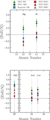 |
Fig. 6 Comparison of mean abundance ratios of EuII relative to other chemical elements for target GCs. The colour coding is the same as in Fig. 3. Error bars indicate the standard deviation. |
5.1 NGC 6218, NGC 6522, NGC 6626, and the Milky Way
We use as a comparison the results obtained from high-resolution spectroscopy of MW field stars, focusing on the chemical elements that show significant differences between accreted and in situ GCs. To do so, given the extremely high quality of their stellar spectra, we selected the catalogue of Nissen & Schuster (2010); Nissen & Schuster (2011) as our benchmark comparison dataset, and in particular we focus on stars in the high-α sequence that have been observed with UVES at the VLT. To maintain homogeneity in the chemical analysis, we re-derived abundances from the spectra of these stars (see the detailed method in Sect. 3). The only exception in this homogeneous comparison is the element EuII, as (i) the number of available spectra in the literature is limited (and many of them were obtained with different instruments and S/N), and (ii) abundances are derived from different spectral lines due to the different evolutionary stages of the observed stars. We chose to compare our results with EuII abundances from the high-α sequence of Fishlock et al. (2017).
Figure 7 shows that the abundances of NGC 6218, NGC 6522, and NGC 6626 match those of the field stars (grey filled points) in all chemical spaces of interest (i.e. Ca, TiI, Zn, YII, and EuII) except for Mg, where the three in situ target GCs show enhancement in [Mg/Fe] compared to MW high-α sequence stars, which is found to be outside the 2σ of their distribution in the metallicity range of −1.3 < [Fe/H] < −1.0 dex.
5.2 NGC 362, NGC 1261, and Gaia-Sausage-Enceladus
The reference catalogue used for this comparison is that of Ceccarelli et al. (2024), which was produced with the same methods as those described here. Additionally, we re-derived the abundances for the stars in the low-α sequence of Nissen & Schuster (2010). Finally, we compared our abundances with the results from the low-α stars in Fishlock et al. (2017); Aguado et al. (2021); Carrillo et al. (2022); Giribaldi & Smiljanic (2023), and François et al. (2024) for EuII. As displayed in Fig. 8, there is excellent agreement between the chemical composition of NGC 362 and NGC 1261 and the patterns shown by GSE stars (grey filled points) in the a-elements Ca and TiI, while, as for in situ GCs, NGC 362 and NGC 1261 lay in the upper boundaries (at the 1.3σ and 1.6σ levels for NGC 362 and NGC 1261, respectively) of the distribution of GSE field stars in [Mg/Fe] in the metallicity range of interest. The value of [Zn/Fe] derived in NGC 1261 is consistent with those observed in the most Zn-poor stars in GSE, while NGC 362 seems to be slightly depleted (~0.1 dex) compared to them. Finally, the slightly subsolar values of [YII/Fe] found for NGC 362 and NGC 1261 are consistent with those observed in the literature (Aguado et al. 2021; Ceccarelli et al. 2024; François et al. 2024), as are the high [EuII/Fe] ratios (see also, Aguado et al. 2021; Matsuno et al. 2021; François et al. 2024; Ou et al. 2024).
This comparison represents strong additional evidence that the two selected GCs were indeed born in the GSE dwarf galaxy, and provides important confirmation that GCs and stars trace the same chemical evolution when sharing the birth environment (see also Monty et al. 2024).
5.3 Ruprecht 106 and the Helmi Streams
In this section, we investigate the compatibility of the chemical composition of Rup106 and that of stars formed in the galaxy that originated the Helmi Streams (Helmi et al. 1999), as a tentative dynamical connection between the two has been pointed out by several works (Massari et al. 2019; Forbes 2020; Callingham et al. 2022). In Fig. 9 we present the mean abundances of Rup106 derived in this work (blue filled squares) compared to the high-resolution abundances of 11 stars linked to the Helmi Streams (grey filled points; Matsuno et al. 2022a, M22 hereafter). We note that we cannot compare EuII abundances as they were not published in M22, and we therefore show Ni as an additional comparison, representative of the iron-peak group. To ensure homogeneity in the comparison, we reanalysed the spectra of the Helmi Streams stars following the procedure described in Sect. 3. The results are shown in Fig. 9 (black filled points). The average offset between our abundances and those of M22 is consistent with zero for all the elements we show in Fig. 9, except for TiI, Ni, and YII, for which we find mild offsets of +0.08 dex (σ = 0.04), −0.08 dex (σ = 0.05), and +0.09 dex (σ = 0.07), respectively. Regardless of the adopted data set (even though the most homogeneous comparison is the one with our reanalysed abundances), when comparing the mean abundance ratios of Rup106 to the trend observed in the Helmi Streams, a noticeable difference emerges, particularly in the α-elements. Our findings consistently indicate [α/Fe] values approximately 0.2 dex lower in comparison to the Helmi Streams, hinting at a lower star formation efficiency in the environment where Rup106 formed. Among the other elements studied, the most significant differences arise in Ni and YII with Rup106 being depleted by ~0.2 dex and by ~0.4 dex, respectively. Therefore, in order to account for the observed differences shown in Fig. 9, the progenitor of the Helmi Streams would need to have been massive enough to be chemically inhomogeneous. Otherwise, this chemical incongruity is strong evidence in support of the interpretation that Rup106 was born in a different environment from the progenitor of the Helmi Streams.
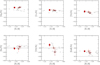 |
Fig. 7 Mean abundances of NGC 6218, NGC 6522, and NGC 6626 derived in this work (the colour coding is the same as in Fig. 3) compared with those derived for MW stars (grey filled points). [EuII/Fe] literature abundances are taken from Fishlock et al. (2017). Error bars show the standard deviation. |
6 Possible origins of Ruprecht 106
In light of the chemical difference between Rup106 and the Helmi Streams stars, and given its peculiar chemical composition compared to many other GCs (e.g. Brown et al. 1997; Carretta et al. 2009, 2013; Villanova et al. 2013; Monaco et al. 2018; Puls et al. 2018; Crestani et al. 2019; Masseron et al. 2019; Horta et al. 2020; Mucciarelli et al. 2021b), the birth environment of Rup106 likely underwent a unique chemical evolution. In the following, we discuss some possible interpretations.
6.1 Comparison with NGC 121
Given its extremely peculiar chemical makeup, Rup106 has long been regarded as originating in an extragalactic environment. Initially, several works proposed that it was likely to have been accreted from the Magellanic Clouds (Lin & Richer 1992; Fusi Pecci et al. 1995), and particularly from the Small Magellanic Cloud (SMC). Although recent post-Gaia kinematics studies of the orbit in the MW of Rup106 (see Sect. 1) have excluded the possibility that it originated in the SMC, it is interesting to note that Rup106 is coeval with NGC 121, the oldest known SMC GC (~ 10.5 Gyr, Glatt et al. 2008; Forbes & Bridges 2010; Dotter et al. 2011) and shows very similar metallicity (Dalessandro et al. 2016; Mucciarelli et al. 2023). Therefore, this presents an excellent opportunity to explore the possibility that an SMC-like galaxy is the progenitor of Rup106. We directly compared our results with those from Mucciarelli et al. (2023), given the congruent analytical approaches. As shown in Fig. 10, NGC 121 (yellow filled squares) has solar-scaled [α/Fe], hinting at an enrichment due to SN Ia already in place in the SMC ~ 10.5 Gyr ago. These values are, on average, 0.1–0.2 dex α-enriched relative to what we find for Rup106, suggesting that Rup106 likely formed in an environment with even less efficient star formation than that of the SMC. Regarding the iron-peak elements, we find comparable values in the abundance ratios of Cu. The very low values of [Cu/Fe] found in both Rup106 and NGC 121 are consistent with those of the SMC field stars (Mucciarelli et al. 2023) and are 0.5 dex underabundant compared to MW GCs and stars, favouring a chemical-enrichment scenario in which the contribution by massive stars is extremely reduced, as also discussed in Sect. 4.2. Additionally, Rup106 shows lower abundances (~0.2 dex) of other elements produced in massive stars (i.e. Sc, V, and Co) relative to NGC 121 and also in Ni. Interestingly, the only elements in which enhancement is detected in Rup106 are Cr and Mn. These elements are predominantly synthesised by SN Ia, with yields depending on the metallicity of the progenitor SN Ia. Unfortunately, Mucciarelli et al. (2023) do not provide an estimate of [Zn/Fe] for NGC 121. When assessing s-process elements, we note similar Ba abundances between the two clusters, yet discern distinct values in Y and La, with Rup106 being, once again, depleted in these elements. Given that NGC 121 demonstrates pronounced deficiencies in these elements relative to the only other SMC GC of similar age, this discrepancy highlights the unique conditions under which Rup106 formed. Also, the efficiency of the production of r-process elements is extremely low, with Rup106 being ~0.7 dex underabundant in Eu relative to NGC 121, which conversely aligns with observations of GSE GCs and SMC stars. This comparison further supports the idea that Rup106 originated in an environment that was significantly different from the SMC of 10.5 Gyr ago and was probably characterised by an exceptionally low star formation efficiency and likely featured a truncated initial mass function (IMF) with a minimal contribution from massive stars.
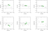 |
Fig. 8 Mean abundances of NGC 362 and NGC 1261 derived in this work (the colour coding is the same as in Fig. 3) compared with those of GSE stars (grey filled points, either derived in this work or by Ceccarelli et al. (2024) for Mg, Ca, TiI, Zn, and YII). Literature abundances for [EuII/Fe] are taken from Fishlock et al. (2017); Aguado et al. (2021); Carrillo et al. (2022); Giribaldi & Smiljanic (2023); François et al. (2024). Error bars stand for the standard deviation. |
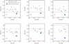 |
Fig. 9 Mean abundances of Rup106 derived in this work (blue filled squares) compared with those derived for field stars associated with the Helmi Streams (results from this work and from M22 are shown in black and grey, respectively). We plot the standard deviation in the bottom left corner. |
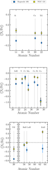 |
Fig. 10 Mean abundances of the α- (top panel), iron-peak (middle panel), and neutron-capture (bottom panel) elements in Rup106 (blue filled squares) and NGC 121 (yellow filled triangles). Error bars indicate the standard deviation. |
6.2 Comparison with surviving dwarf galaxies
A similar chemical composition to that of Rup106 has been observed in stars belonging to dwarf galaxies in the Local Group (Venn et al. 2004; Tolstoy et al. 2009). Indeed, subsolar [α/Fe] values at [Fe/H] ≤ − 1.5 dex are observed in surviving dwarf galaxies such as Carina, Fornax, Sculptor, Sextans, and Ursa Minor (Venn et al. 2012; Hendricks et al. 2014; Hill et al. 2019; Theler et al. 2020; Fernandes et al. 2023; Sestito et al. 2023). The low values of Zn ([Zn/Fe] ~ −0.3 dex) derived for Rup106 compared to those found in MW stars are also typical of these systems (see Fig. 16 of Skúladóttir et al. 2017, and reference therein). Finally, most of the dwarf galaxies show enhancement in [EuII/Fe] compared to MW stars due to either the very low star formation efficiency or the delayed contribution to the production of Eu by NSMs (Letarte et al. 2010; Venn et al. 2012; Lemasle et al. 2014). However, even the extremely low [EuII/Fe] of Rup106 can be reproduced in some of these systems, such as Sculptor (Hill et al. 2019). Indeed, these latter authors find several stars in Sculptor with subsolar values (~ − 0.1 dex) of [EuII/BaII] at [Fe/H] ~ − 1.3 dex , suggesting that the onset of s-process enrichment was already in place at this metallicity. It is interesting to note that the chemical composition of Rup106 resembles that found in iron-rich metal-poor stars (IRMP), despite these latter being unlikely to form in GCs, thus indicating a birth environment enriched by the (double) detonation of sub-Chandrasekhar-mass CO white dwarfs (Reggiani et al. 2023). This further supports the idea that Rup106 formed in a dwarf galaxy, as these authors demonstrated that IRMP stars are easier to find in surviving dwarf galaxies and the Magellanic Clouds, rather than in the halo of the MW.
It is important to note that the majority of the existing systems that reproduce the peculiar chemistry of Rup106 have a stellar mass (~106 M⊙, McConnachie 2012) that is not compatible with that estimated for the progenitor of the Helmi Streams, with the latter being roughly 100 times more massive (Koppelman et al. 2019). Therefore, if the dynamical association of Rup106 is accurate, the possibility that it did not form directly in the progenitor of the Helmi Streams cannot be ruled out. We speculate that Rup106 could have formed in a dwarf galaxy with a mass comparable to that of Sculptor; the dynamical properties of Rup106 suggest that this could have been a satellite of the progenitor of the Helmi Streams or the Sagittarius dwarf (Davies et al. 2024), similarly to the case of the GC NGC 2005 in the Large Magellanic Cloud (Mucciarelli et al. 2021b).
7 Conclusion
The primary aim of this work is to investigate the potential differences in elemental abundances between six GCs of very similar metallicity (−1.3 ≤ [Fe/H] ≤ −1.0 dex) that are expected to have formed in different environments, and to decipher which abundance ratios are most sensitive to their different origin.
The outcome of this homogeneous chemical analysis reveals striking similarities in the chemical abundances of NGC 362 and NGC 1261, two GCs that were accreted during the merger event of the Gaia-Sausage-Enceladus dwarf galaxy. When comparing the chemical abundances of these GCs with those of the in situ GCs NGC 6218, NGC 6522, and NGC 6626, a coherent and distinct overall pattern emerges in the α-elements, especially in Mg, Si, and Ca, where we identify a depletion of ~0.1 dex in the GSE GCs with respect to in situ GCs. This finding agrees with observations of field stars of the Galactic halo in this metallic-ity range, where distinctions between chemical patterns of in situ and accreted stars are discernible, especially in the α-elements, whereas trends become indistinguishable at lower metallicity (Horta et al. 2023; Ceccarelli et al. 2024). This is consistent with the fact that it took 2 Gyr less for NGC 6218, NGC 6522, and NGC 6626 to reach the same metallicity as the GSE GCs (Dotter et al. 2010; Dotter et al. 2011; VandenBerg et al. 2013; Villanova et al. 2017; Kerber et al. 2018), indicating that the contribution of SN Ia to the chemical enrichment of the gas was not in place at the time when these systems formed. Moreover, statistically significant variations are observed in specific elements such as Zn and Eu, whose production sites are directly associated with massive stars (HNe for Zn and rCCSNe+NSMs for Eu). It is worth noting that that these events are inherently rare, and might exert a profound influence on the abundances within a given environment. These results reinforce the idea that chemical tagging is an effective tool for investigating the origin of GCs, even when comparing the chemical compositions of GCs formed in different progenitors, but at the same time demonstrate that not every element is equally sensitive in this sense.
In this coherent picture, Rup106 stands out as a highly distinct GC. Indeed, Rup106 follows the AMR of accreted GCs (Forbes & Bridges 2010; Dotter et al. 2010; Dotter et al. 2011; VandenBerg et al. 2013), whereas MW in situ clusters of similar age clearly experienced a different chemical enrichment path, exhibiting significantly higher metallicity (0.5–0.8 dex more metal rich; Massari et al. 2023). Despite the congruence between Rup106 and the GSE GCs in the age-metallicity space, differences emerge when examining all their chemical elements. Particularly, Rup106 exhibits subsolar [α/Fe] values typical of an environment already enriched by SNe Ia, in contrast to GSE clusters ([α/Fe] > 0.3 dex), where SNe Ia have only just started contributing to the enrichment of the gas. This comparison underlines distinct chemical evolution histories between GSE and the environment in which Rup106 formed, with the latter experiencing slower and less efficient star formation and likely an IMF truncated of most of the massive stars, indicating a lower mass for the host of Rup106 at ~ 10.5 Gyr ago compared to GSE.
In light of these results, this work demonstrates that the exceptionally high precision offered by a strictly homogeneous chemical analysis allows chemical tagging to play a crucial role in uncovering the true origin of GCs. Particularly, this method enables us not only to clearly discriminate between GCs formed within the MW and those formed in other accreted galaxies, but also to distinguish the chemical signatures of GCs originating from independent accreted progenitors.
Finally, we interpret the extreme peculiarity of the chemistry of Rup106 as due to the particular evolution of its progenitor, which could be the galaxy that gave rise to the Helmi Streams. However, the remarkably low values of the [α/Fe] abundance ratios, as well as of some other heavier elements, compared to Helmi Streams stars lend weight to the possibility that Rup106 originated from an even smaller galaxy, with a stellar mass comparable to that of some surviving dwarf galaxies (e.g. Sculptor).
Data availability
Table B.1 with information on the line list used in this work is available on Zenodo at https://doi.org/10.5281/zenodo.13907515.
The Full Tables 1-4 is also available at the CDS via anonymous ftp to cdsarc.cds.unistra.fr (130.79.128.5) or via https://cdsarc.cds.unistra.fr/viz-bin/cat/J/A+A/691/A226
Acknowledgements
Based on observations collected at the ESO-VLT under the programs 069.D-0227 (P.I. P. Francois), 073.D-0211 (P.I. E. Carretta), 083.D-0208 (P.I. E. Carretta), 091.D-0535 (PI: C. Moni Bidin), 097.D-0175 (PI: B. Barbuy), 0101.D-0109 (P.I. A. Marino), 193.D-0232 (P.I. F. R. Fer-raro), and 197.B-1074 (P.I. G. F. Gilmore). This research is funded by the project LEGO — Reconstructing the building blocks of the Galaxy by chemical tagging (P.I. A. Mucciarelli), granted by the Italian MUR through contract PRIN 2022LLP8TK_001. MB, EC, AM and DM acknowledge the support to this study by the PRIN INAF 2023 grant ObFu CHAM — Chemodynamics of the Accreted Halo of the Milky Way (P.I. M. Bellazzini). DM acknowledges financial support from PRIN-MIUR-22 “CHRONOS: adjusting the clock(s) to unveil the CHRONO-chemo-dynamical Structure of the Galaxy” (PI: S. Cassisi) granted by the European Union - Next Generation EU. DM and MB acknowledge the support to activities related to the ESA/Gaia mission by the Italian Space Agency (ASI) through contract 2018-24-HH.0 and its addendum 2018-24-HH.1-2022 to the National Institute for Astrophysics (INAF). We thank the anonymous referee for the helpful comments that improved the quality of the paper. This work has made use of data from the European Space Agency (ESA) mission Gaia (https://www.cosmos.esa.int/gaia), processed by the Gaia Data Processing and Analysis Consortium (DPAC, https://www.cosmos.esa.int/web/gaia/dpac/consortium). Funding for the DPAC has been provided by national institutions, in particular the institutions participating in the Gaia Multilateral Agreement. This work made use of SDSS-IV data. Funding for the Sloan Digital Sky Survey IV has been provided by the Alfred P. Sloan Foundation, the U.S. Department of Energy Office of Science, and the Participating Institutions. SDSS-IV acknowledges support and resources from the Center for High Performance Computing at the University of Utah. The SDSS website is www.sdss4.org. SDSS-IV is managed by the Astrophysical Research Consortium for the Participating Institutions of the SDSS Collaboration including the Brazilian Participation Group, the Carnegie Institution for Science, Carnegie Mellon University, Center for Astrophysics | Harvard & Smithsonian, the Chilean Participation Group, the French Participation Group, Instituto de Astrofísica de Canarias, The Johns Hopkins University, Kavli Institute for the Physics and Mathematics of the Universe (IPMU) / University of Tokyo, the Korean Participation Group, Lawrence Berkeley National Laboratory, Leibniz Institut für Astrophysik Potsdam (AIP), Max-Planck-Institut für Astronomie (MPIA Heidelberg), Max-Planck-Institut für Astrophysik (MPA Garching), Max-Planck-Institut für Extraterrestrische Physik (MPE), National Astronomical Observatories of China, New Mexico State University, New York University, University of Notre Dame, Observatário Nacional / MCTI, The Ohio State University, Pennsylvania State University, Shanghai Astronomical Observatory, United Kingdom Participation Group, Universidad Nacional Autónoma de Mexico, University of Arizona, University of Colorado Boulder, University of Oxford, University of Portsmouth, University of Utah, University of Virginia, University of Washington, University of Wisconsin, Vanderbilt University, and Yale University.
Appendix A Validation of the abundances
A.1 GSE globular clusters
To validate our findings, we undertake a comparative analysis with two distinct independent studies conducted on two of the six target GCs. Specifically, we compare our results to those obtained by the seminal works by Carretta et al. (2009, 2010, 2013) and to those provided by the latest data release of the APOGEE survey (Abdurro’uf et al. 2022). In particular, we use the APOGEE value-added catalogue of Galactic GC stars (Schiavon et al. 2024), limiting our comparison only to well-measured stars. To do so, we remove all the stars with the following flags3 in the quality parameters:
ASPCAPFLAG = 16, 17, 23;
STARFLAG = 3, 4, 9, 12, 13, 16;
EXTRATARG = 4;
VB_PROB > 0.99.
The choice of using these two dataset was guided by their execution of identical chemical analyses on two out of the four target GCs, thereby ensuring consistency in their outcomes. We limit our comparison with Carretta et al. (2009, 2010, 2013) and APOGEE only to the chemical elements identified as sensitive to the origin of GCs available in these dataset, that are Mg, Si and Ca. As shown in Fig. A.1, the results from this work are in agreement within the uncertainties with those provided by Carretta et al. (2009, 2010, 2013) and APOGEE, consistently yielding an enhancement of 0.1 - 0.2 dex in the α-elements (Mg, Si, and Ca) of NGC 6218 with respect to NGC 362.
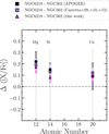 |
Fig. A.1 Difference of mean abundance ratios of the α-elements [Mg/Fe], [Si/Fe], and [Ca/Fe] between NGC 6218 and NGC 362 from this work (pink triangles), Carretta et al. (2009, 2010, 2013) (purple squares), and APOGEE (black squares). Error bars indicate the standard deviation. |
A.2 Comparison with V13
A comparison with the results of V13, who analyzed the same Rup106 dataset, further confirms the peculiarity of this system. Indeed, their findings indicate that, within this cluster, the observed spread in all chemical elements is consistent with the uncertainty on the measurement, suggesting Rup106 to be a single population GC, as also confirmed photometrically in more recent works (Dotter et al. 2018; Lagioia et al. 2024). Moreover, their analysis reveals solar-like abundances in the α-elements, alongside a notable underabundance in the iron peak elements relative to iron, ranging from 0.1 up to 0.8 dex. Firstly, when comparing the atmospheric parameters of Rup106 targets, we find a significant difference in the adopted Teff scales, with an average discrepancy (this work − V13) of +169 K (σ = 55 K). The average difference for the surface gravity is +0.65 dex (σ = 0.14 dex) and that for vt is −0.07 km/s (σ = 0.05 km/s). These discrepancies arise from the fact that V13 constrained Teff and log ɡ with a metodology similar to ours, deriving them from the photometry, but exploiting a different colour - Teff relation. On the other hand, V13 assumed a vt derived from the relation by Marino et al. (2008), while we constrained it spectroscopi-cally (see Sect. 3.1). To ensure a fair comparison between the results, we rescaled the abundance ratios reported in V13 on the Grevesse & Sauval (1998) solar composition. Firstly, we note an average offset of +0.17 dex (σ = 0.07 dex) in the star-to-star metallicity estimate of Rup106, which can be explained by the difference in the derived effective temperatures. By comparing these two independent results performed on the same dataset, we find agreement with V13 at the 1σ level for Mg, Ti, ScII, Cr, Mn, Zn, YII, LaII, and EuII, while we note differences up to ~ 0.2 dex for Si, Ca, V, Co, Ni, Cu, and BaII. We attribute these inconsistencies to the different scale adopted for surface gravities and, most importantly, effective temperatures. This comparison proves that diverse assumptions in the procedure to derive chemical abundances make the results of two independent approaches not directly comparable and that the only reliable chemical analysis is within an homogeneous procedure. In general, notwithstanding differences stemming from varied assumptions in the chemical analysis, we reaffirm the distinct chemical characteristics of Rup106 within the MW GC system, alongside the minimal dispersion in chemical abundances among its constituent stars.
Appendix B Line list
In Table B.1, we list some useful information about the lines analyzed using the EW method, such as the wavelength, the log gf, the excitation potential (χ) and the EW measured with the code DAOSPEC.
Lines analyzed in this work for each star (extract).
References
- Abdurro’uf, Accetta, K., Aerts, C., et al. 2022, ApJS, 259, 35 [NASA ADS] [CrossRef] [Google Scholar]
- Aguado, D. S., Belokurov, V., Myeong, G. C., et al. 2021, ApJ, 908, L8 [NASA ADS] [CrossRef] [Google Scholar]
- Alvarez Garay, D. A., Mucciarelli, A., Bellazzini, M., Lardo, C., & Ventura, P. 2024, A&A, 681, A54 [NASA ADS] [CrossRef] [EDP Sciences] [Google Scholar]
- Amarante, J. A. S., Debattista, V. P., Beraldo e Silva, L., Laporte, C. F. P., & Deg, N. 2022, ApJ, 937, 12 [NASA ADS] [CrossRef] [Google Scholar]
- Andrae, R., Fouesneau, M., Creevey, O., et al. 2018, A&A, 616, A8 [NASA ADS] [CrossRef] [EDP Sciences] [Google Scholar]
- Barbuy, B., Cantelli, E., Muniz, L., et al. 2021, A&A, 654, A29 [NASA ADS] [CrossRef] [EDP Sciences] [Google Scholar]
- Bastian, N., & Lardo, C. 2018, ARA&A, 56, 83 [Google Scholar]
- Baumgardt, H., & Vasiliev, E. 2021, MNRAS, 505, 5957 [NASA ADS] [CrossRef] [Google Scholar]
- Bellazzini, M., Ibata, R., Malhan, K., et al. 2020, A&A, 636, A107 [NASA ADS] [CrossRef] [EDP Sciences] [Google Scholar]
- Belokurov, V., & Kravtsov, A. 2022, MNRAS, 514, 689 [NASA ADS] [CrossRef] [Google Scholar]
- Belokurov, V., & Kravtsov, A. 2024, MNRAS, 528, 3198 [CrossRef] [Google Scholar]
- Belokurov, V., Erkal, D., Evans, N. W., Koposov, S. E., & Deason, A. J. 2018, MNRAS, 478, 611 [Google Scholar]
- Belokurov, V., Vasiliev, E., Deason, A. J., et al. 2023, MNRAS, 518, 6200 [Google Scholar]
- Brodie, J. P., & Strader, J. 2006, ARA&A, 44, 193 [Google Scholar]
- Brown, J. A., Wallerstein, G., & Zucker, D. 1997, AJ, 114, 180 [NASA ADS] [CrossRef] [Google Scholar]
- Callingham, T. M., Cautun, M., Deason, A. J., et al. 2022, MNRAS, 513, 4107 [NASA ADS] [CrossRef] [Google Scholar]
- Cardelli, J. A., Clayton, G. C., & Mathis, J. S. 1989, ApJ, 345, 245 [Google Scholar]
- Carretta, E., Bragaglia, A., Gratton, R., & Lucatello, S. 2009, A&A, 505, 139 [NASA ADS] [CrossRef] [EDP Sciences] [Google Scholar]
- Carretta, E., Bragaglia, A., Gratton, R., et al. 2010, ApJ, 712, L21 [NASA ADS] [CrossRef] [Google Scholar]
- Carretta, E., Bragaglia, A., Gratton, R. G., et al. 2013, A&A, 557, A138 [NASA ADS] [CrossRef] [EDP Sciences] [Google Scholar]
- Carrillo, A., Hawkins, K., Jofré, P., et al. 2022, MNRAS, 513, 1557 [CrossRef] [Google Scholar]
- Castelli, F., & Kurucz, R. L. 2003, in Modelling of Stellar Atmospheres, 210, eds. N. Piskunov, W. W. Weiss, & D. F. Gray, A20 [NASA ADS] [Google Scholar]
- Ceccarelli, E., Massari, D., Mucciarelli, A., et al. 2024, A&A, 684, A37 [NASA ADS] [CrossRef] [EDP Sciences] [Google Scholar]
- Cescutti, G., Romano, D., Matteucci, F., Chiappini, C., & Hirschi, R. 2015, A&A, 577, A139 [NASA ADS] [CrossRef] [EDP Sciences] [Google Scholar]
- Chen, Y., & Gnedin, O. Y. 2024, Open J. Astrophys., 7, 23 [NASA ADS] [Google Scholar]
- Crestani, J., Alves-Brito, A., Bono, G., Puls, A. A., & Alonso-García, J. 2019, MNRAS, 487, 5463 [Google Scholar]
- Dalessandro, E., Lapenna, E., Mucciarelli, A., et al. 2016, ApJ, 829, 77 [NASA ADS] [CrossRef] [Google Scholar]
- Davies, E. Y., Monty, S., Belokurov, V., & Dillamore, A. M. 2024, MNRAS, 529, 772 [NASA ADS] [CrossRef] [Google Scholar]
- Dekker, H., D’Odorico, S., Kaufer, A., Delabre, B., & Kotzlowski, H. 2000, SPIE Conf. Ser., 4008, 534 [Google Scholar]
- Dell’Agli, F., García-Hernández, D. A., Ventura, P., et al. 2018, MNRAS, 475, 3098 [CrossRef] [Google Scholar]
- Dotter, A., Sarajedini, A., Anderson, J., et al. 2010, ApJ, 708, 698 [Google Scholar]
- Dotter, A., Sarajedini, A., & Anderson, J. 2011, ApJ, 738, 74 [NASA ADS] [CrossRef] [Google Scholar]
- Dotter, A., Milone, A. P., Conroy, C., Marino, A. F., & Sarajedini, A. 2018, ApJ, 865, L10 [NASA ADS] [CrossRef] [Google Scholar]
- Fernandes, L., Mason, A. C., Horta, D., et al. 2023, MNRAS, 519, 3611 [NASA ADS] [CrossRef] [Google Scholar]
- Fishlock, C. K., Yong, D., Karakas, A. I., et al. 2017, MNRAS, 466, 4672 [NASA ADS] [Google Scholar]
- Forbes, D. A. 2020, MNRAS, 493, 847 [Google Scholar]
- Forbes, D. A., & Bridges, T. 2010, MNRAS, 404, 1203 [NASA ADS] [Google Scholar]
- François, P., Cescutti, G., Bonifacio, P., et al. 2024, A&A, 686, A295 [NASA ADS] [CrossRef] [EDP Sciences] [Google Scholar]
- Frelijj, H., Villanova, S., Muñoz, C., & Fernández-Trincado, J. G. 2021, MNRAS, 503, 867 [NASA ADS] [CrossRef] [Google Scholar]
- Fusi Pecci, F., Bellazzini, M., Cacciari, C., & Ferraro, F. R. 1995, AJ, 110, 1664 [NASA ADS] [CrossRef] [Google Scholar]
- Gaia Collaboration (Babusiaux, C., et al.) 2018, A&A, 616, A10 [NASA ADS] [CrossRef] [EDP Sciences] [Google Scholar]
- Gaia Collaboration (Brown, A. G. A., et al.) 2021, A&A, 649, A1 [NASA ADS] [CrossRef] [EDP Sciences] [Google Scholar]
- Gaia Collaboration (Vallenari, A., et al.) 2023, A&A, 674, A1 [NASA ADS] [CrossRef] [EDP Sciences] [Google Scholar]
- Giribaldi, R. E., & Smiljanic, R. 2023, A&A, 673, A18 [NASA ADS] [CrossRef] [EDP Sciences] [Google Scholar]
- Glatt, K., Gallagher, I., John S., Grebel, E. K., et al. 2008, AJ, 135, 1106 [NASA ADS] [CrossRef] [Google Scholar]
- Grevesse, N., & Sauval, A. J. 1998, Space Sci. Rev., 85, 161 [Google Scholar]
- Harris, W. E. 2010, arXiv e-prints [arXiv:1012.3224] [Google Scholar]
- Helmi, A. 2020, ARA&A, 58, 205 [Google Scholar]
- Helmi, A., & de Zeeuw, P. T. 2000, MNRAS, 319, 657 [Google Scholar]
- Helmi, A., White, S. D. M., de Zeeuw, P. T., & Zhao, H. 1999, Nature, 402, 53 [Google Scholar]
- Helmi, A., Babusiaux, C., Koppelman, H. H., et al. 2018, Nature, 563, 85 [Google Scholar]
- Hendricks, B., Koch, A., Walker, M., et al. 2014, A&A, 572, A82 [NASA ADS] [CrossRef] [EDP Sciences] [Google Scholar]
- Hill, V., Skúladóttir, Á., Tolstoy, E., et al. 2019, A&A, 626, A15 [NASA ADS] [CrossRef] [EDP Sciences] [Google Scholar]
- Horta, D., Schiavon, R. P., Mackereth, J. T., et al. 2020, MNRAS, 493, 3363 [NASA ADS] [CrossRef] [Google Scholar]
- Horta, D., Schiavon, R. P., Mackereth, J. T., et al. 2023, MNRAS, 520, 5671 [NASA ADS] [CrossRef] [Google Scholar]
- Ibata, R. A., Gilmore, G., & Irwin, M. J. 1994, Nature, 370, 194 [Google Scholar]
- Ibata, R., Malhan, K., Tenachi, W., et al. 2024, ApJ, 967, 89 [NASA ADS] [CrossRef] [Google Scholar]
- Kerber, L. O., Nardiello, D., Ortolani, S., et al. 2018, ApJ, 853, 15 [Google Scholar]
- Kobayashi, C., & Nomoto, K. 2009, ApJ, 707, 1466 [NASA ADS] [CrossRef] [Google Scholar]
- Kobayashi, C., Karakas, A. I., & Lugaro, M. 2020, ApJ, 900, 179 [Google Scholar]
- Koch-Hansen, A. J., Hansen, C. J., & McWilliam, A. 2021, A&A, 653, A2 [NASA ADS] [CrossRef] [EDP Sciences] [Google Scholar]
- Koppelman, H. H., Helmi, A., Massari, D., Price-Whelan, A. M., & Starkenburg, T. K. 2019, A&A, 631, L9 [NASA ADS] [CrossRef] [EDP Sciences] [Google Scholar]
- Kruijssen, J. M. D., Pfeffer, J. L., Reina-Campos, M., Crain, R. A., & Bastian, N. 2019, MNRAS, 486, 3180 [Google Scholar]
- Kurucz, R. L. 2005, Mem. Soc. Astron. Ital. Suppl., 8, 14 [Google Scholar]
- Lagioia, E. P., Milone, A. P., Legnardi, M. V., et al. 2024, arXiv e-prints [arXiv:2406.16824] [Google Scholar]
- Lattimer, J. M., & Schramm, D. N. 1974, ApJ, 192, L145 [NASA ADS] [CrossRef] [Google Scholar]
- Leaman, R., VandenBerg, D. A., & Mendel, J. T. 2013, MNRAS, 436, 122 [Google Scholar]
- Lemasle, B., de Boer, T. J. L., Hill, V., et al. 2014, A&A, 572, A88 [NASA ADS] [CrossRef] [EDP Sciences] [Google Scholar]
- Letarte, B., Hill, V., Tolstoy, E., et al. 2010, A&A, 523, A17 [NASA ADS] [CrossRef] [EDP Sciences] [Google Scholar]
- Limberg, G., Souza, S. O., Pérez-Villegas, A., et al. 2022, ApJ, 935, 109 [NASA ADS] [CrossRef] [Google Scholar]
- Lin, D. N. C., & Richer, H. B. 1992, ApJ, 388, L57 [NASA ADS] [CrossRef] [Google Scholar]
- Lucertini, F., Monaco, L., Caffau, E., et al. 2023, A&A, 671, A137 [NASA ADS] [CrossRef] [EDP Sciences] [Google Scholar]
- Majewski, S. R., Skrutskie, M. F., Weinberg, M. D., & Ostheimer, J. C. 2003, ApJ, 599, 1082 [NASA ADS] [CrossRef] [Google Scholar]
- Malhan, K., Ibata, R. A., Sharma, S., et al. 2022, ApJ, 926, 107 [NASA ADS] [CrossRef] [Google Scholar]
- Marín-Franch, A., Aparicio, A., Piotto, G., et al. 2009, ApJ, 694, 1498 [Google Scholar]
- Marino, A. F., Villanova, S., Piotto, G., et al. 2008, A&A, 490, 625 [NASA ADS] [CrossRef] [EDP Sciences] [Google Scholar]
- Marino, A. F., Milone, A. P., Renzini, A., et al. 2021, ApJ, 923, 22 [CrossRef] [Google Scholar]
- Massari, D., Koppelman, H. H., & Helmi, A. 2019, A&A, 630, L4 [NASA ADS] [CrossRef] [EDP Sciences] [Google Scholar]
- Massari, D., Aguado-Agelet, F., Monelli, M., et al. 2023, A&A, 680, A20 [NASA ADS] [CrossRef] [EDP Sciences] [Google Scholar]
- Masseron, T., García-Hernández, D. A., Mészáros, S., et al. 2019, A&A, 622, A191 [NASA ADS] [CrossRef] [EDP Sciences] [Google Scholar]
- Matsuno, T., Hirai, Y., Tarumi, Y., et al. 2021, A&A, 650, A110 [NASA ADS] [CrossRef] [EDP Sciences] [Google Scholar]
- Matsuno, T., Dodd, E., Koppelman, H. H., et al. 2022a, A&A, 665, A46 [NASA ADS] [CrossRef] [EDP Sciences] [Google Scholar]
- Matsuno, T., Koppelman, H. H., Helmi, A., et al. 2022b, A&A, 661, A103 [NASA ADS] [CrossRef] [EDP Sciences] [Google Scholar]
- McConnachie, A. W. 2012, AJ, 144, 4 [Google Scholar]
- Milone, A. P., Piotto, G., Bedin, L. R., et al. 2012, A&A, 540, A16 [NASA ADS] [CrossRef] [EDP Sciences] [Google Scholar]
- Minelli, A., Mucciarelli, A., Massari, D., et al. 2021, ApJ, 918, L32 [NASA ADS] [CrossRef] [Google Scholar]
- Monaco, L., Villanova, S., Carraro, G., Mucciarelli, A., & Moni Bidin, C. 2018, A&A, 616, A181 [NASA ADS] [CrossRef] [EDP Sciences] [Google Scholar]
- Monty, S., Yong, D., Marino, A. F., et al. 2023a, MNRAS, 518, 965 [Google Scholar]
- Monty, S., Yong, D., Massari, D., et al. 2023b, MNRAS, 522, 4404 [NASA ADS] [CrossRef] [Google Scholar]
- Monty, S., Belokurov, V., Sanders, J. L., et al. 2024, MNRAS, 533, 2420 [NASA ADS] [CrossRef] [Google Scholar]
- Moore, B., Ghigna, S., Governato, F., et al. 1999, ApJ, 524, L19 [Google Scholar]
- Mösta, P., Roberts, L. F., Halevi, G., et al. 2018, ApJ, 864, 171 [Google Scholar]
- Mucciarelli, A. 2013, arXiv e-prints [arXiv:1311.1403] [Google Scholar]
- Mucciarelli, A., Pancino, E., Lovisi, L., Ferraro, F. R., & Lapenna, E. 2013, ApJ, 766, 78 [NASA ADS] [CrossRef] [Google Scholar]
- Mucciarelli, A., Bellazzini, M., & Massari, D. 2021a, A&A, 653, A90 [NASA ADS] [CrossRef] [EDP Sciences] [Google Scholar]
- Mucciarelli, A., Massari, D., Minelli, A., et al. 2021b, Nat. Astron., 5, 1247 [NASA ADS] [CrossRef] [Google Scholar]
- Mucciarelli, A., Minelli, A., Lardo, C., et al. 2023, A&A, 677, A61 [NASA ADS] [CrossRef] [EDP Sciences] [Google Scholar]
- Myeong, G. C., Evans, N. W., Belokurov, V., Sanders, J. L., & Koposov, S. E. 2018, ApJ, 856, L26 [NASA ADS] [CrossRef] [Google Scholar]
- Myeong, G. C., Vasiliev, E., Iorio, G., Evans, N. W., & Belokurov, V. 2019, MNRAS, 488, 1235 [Google Scholar]
- Naidu, R. P., Conroy, C., Bonaca, A., et al. 2022a, arXiv e-prints [arXiv:2204.09057] [Google Scholar]
- Naidu, R. P., Ji, A. P., Conroy, C., et al. 2022b, ApJ, 926, L36 [CrossRef] [Google Scholar]
- Newton, O., Cautun, M., Jenkins, A., Frenk, C. S., & Helly, J. C. 2018, MNRAS, 479, 2853 [CrossRef] [Google Scholar]
- Nissen, P. E., & Schuster, W. J. 2010, A&A, 511, L10 [NASA ADS] [CrossRef] [EDP Sciences] [Google Scholar]
- Nissen, P. E., & Schuster, W. J. 2011, A&A, 530, A15 [NASA ADS] [CrossRef] [EDP Sciences] [Google Scholar]
- Ou, X., Ji, A. P., Frebel, A., Naidu, R. P., & Limberg, G. 2024, arXiv e-prints [arXiv:2404.10067] [Google Scholar]
- Pagnini, G., Di Matteo, P., Khoperskov, S., et al. 2023, A&A, 673, A86 [NASA ADS] [CrossRef] [EDP Sciences] [Google Scholar]
- Pasquini, L., Avila, G., Blecha, A., et al. 2002, The Messenger, 110, 1 [Google Scholar]
- Peñarrubia, J., Walker, M. G., & Gilmore, G. 2009, MNRAS, 399, 1275 [CrossRef] [Google Scholar]
- Puls, A. A., Alves-Brito, A., Campos, F., Dias, B., & Barbuy, B. 2018, MNRAS, 476, 690 [NASA ADS] [CrossRef] [Google Scholar]
- Recio-Blanco, A. 2018, A&A, 620, A194 [NASA ADS] [CrossRef] [EDP Sciences] [Google Scholar]
- Reggiani, H., Schlaufman, K. C., & Casey, A. R. 2023, AJ, 166, 128 [NASA ADS] [CrossRef] [Google Scholar]
- Romano, D., Karakas, A. I., Tosi, M., & Matteucci, F. 2010, A&A, 522, A32 [NASA ADS] [CrossRef] [EDP Sciences] [Google Scholar]
- Schiavon, R. P., Phillips, S. G., Myers, N., et al. 2024, MNRAS, 528, 1393 [CrossRef] [Google Scholar]
- Sestito, F., Zaremba, D., Venn, K. A., et al. 2023, MNRAS, 525, 2875 [NASA ADS] [CrossRef] [Google Scholar]
- Siegel, D. M., Barnes, J., & Metzger, B. D. 2019, Nature, 569, 241 [Google Scholar]
- Skúladóttir, Á., Tolstoy, E., Salvadori, S., Hill, V., & Pettini, M. 2017, A&A, 606, A71 [NASA ADS] [CrossRef] [EDP Sciences] [Google Scholar]
- Stetson, P. B., & Pancino, E. 2008, PASP, 120, 1332 [Google Scholar]
- Theler, R., Jablonka, P., Lucchesi, R., et al. 2020, A&A, 642, A176 [NASA ADS] [CrossRef] [EDP Sciences] [Google Scholar]
- Tolstoy, E., Hill, V., & Tosi, M. 2009, ARA&A, 47, 371 [Google Scholar]
- Trujillo-Gomez, S., Kruijssen, J. M. D., Reina-Campos, M., et al. 2021, MNRAS, 503, 31 [NASA ADS] [CrossRef] [Google Scholar]
- VandenBerg, D. A., Brogaard, K., Leaman, R., & Casagrande, L. 2013, ApJ, 775, 134 [Google Scholar]
- Van der Swaelmen, M., Hill, V., Primas, F., & Cole, A. A. 2013, A&A, 560, A44 [NASA ADS] [CrossRef] [EDP Sciences] [Google Scholar]
- Vasiliev, E., & Baumgardt, H. 2021, MNRAS, 505, 5978 [NASA ADS] [CrossRef] [Google Scholar]
- Venn, K. A., Irwin, M., Shetrone, M. D., et al. 2004, AJ, 128, 1177 [NASA ADS] [CrossRef] [Google Scholar]
- Venn, K. A., Shetrone, M. D., Irwin, M. J., et al. 2012, ApJ, 751, 102 [Google Scholar]
- Ventura, P., Di Criscienzo, M., Carini, R., & D’Antona, F. 2013, MNRAS, 431, 3642 [Google Scholar]
- Villanova, S., Geisler, D., Carraro, G., Moni Bidin, C., & Muñoz, C. 2013, ApJ, 778, 186 [Google Scholar]
- Villanova, S., Moni Bidin, C., Mauro, F., Munoz, C., & Monaco, L. 2017, MNRAS, 464, 2730 [Google Scholar]
- White, S. D. M., & Frenk, C. S. 1991, ApJ, 379, 52 [Google Scholar]
- Yan, Z., Jerabkova, T., & Kroupa, P. 2020, A&A, 637, A68 [NASA ADS] [CrossRef] [EDP Sciences] [Google Scholar]
Flags definition available at https://www.sdss4.org/dr17/irspec/apogee-bitmasks/.
All Tables
Chemical abundances for the neutron-capture elements for the target stars (extract).
All Figures
|
Fig. 1 Spectra of stars from the six target clusters observed with UVES and UVES-FLAMES at the VLT at different wavelengths. The spectra have been vertically shifted for the sake of clarity. |
| In the text | |
|
Fig. 2 Comparison around the 4810.5 Å Zn (left panel) and the 6645.1 Å EuII (right panel) lines between the observed spectra and seven synthetic spectra computed assuming the derived atmospheric parameters for each star and varying the level of [Zn/Fe] and [EuII/Fe]. The variations are computed with respect to the abundances measured in Rup106. |
| In the text | |
|
Fig. 3 Comparison of mean abundance ratios of the α-elements [Mg/Fe], [Si/Fe], [Ca/Fe], [Til/Fe], and [Till/Fe] for target GCs NGC 362 (green triangles), NGC 1261 (dark green circles), NGC 6218 (red squares), NGC 6522 (brown trianges), NGC 6626 (pink triangles), and Rup106 (blue squares). Error bars indicate the standard deviation. |
| In the text | |
|
Fig. 4 Comparison of mean abundance ratios of the iron-peak elements [ScII/Fe], [V/Fe], [Cr/Fe], [Mn/Fe], [Co/Fe], [Ni/Fe], and [Zn/Fe] for target GCs (top panel). In the bottom panel we plot the two elements ([Cu/Fe] and [YII/Fe]) with the largest differences observed for Rup106. The colour coding is the same as in Fig. 3. Error bars indicate the standard deviation. |
| In the text | |
|
Fig. 5 Comparison of mean abundance ratios of the neutron-capture elements [BaII/Fe], [LaII/Fe], and [EuII/Fe] for our target GCs. The colour coding is the same as in Fig. 3. Error bars indicate the standard deviation. |
| In the text | |
|
Fig. 6 Comparison of mean abundance ratios of EuII relative to other chemical elements for target GCs. The colour coding is the same as in Fig. 3. Error bars indicate the standard deviation. |
| In the text | |
|
Fig. 7 Mean abundances of NGC 6218, NGC 6522, and NGC 6626 derived in this work (the colour coding is the same as in Fig. 3) compared with those derived for MW stars (grey filled points). [EuII/Fe] literature abundances are taken from Fishlock et al. (2017). Error bars show the standard deviation. |
| In the text | |
|
Fig. 8 Mean abundances of NGC 362 and NGC 1261 derived in this work (the colour coding is the same as in Fig. 3) compared with those of GSE stars (grey filled points, either derived in this work or by Ceccarelli et al. (2024) for Mg, Ca, TiI, Zn, and YII). Literature abundances for [EuII/Fe] are taken from Fishlock et al. (2017); Aguado et al. (2021); Carrillo et al. (2022); Giribaldi & Smiljanic (2023); François et al. (2024). Error bars stand for the standard deviation. |
| In the text | |
|
Fig. 9 Mean abundances of Rup106 derived in this work (blue filled squares) compared with those derived for field stars associated with the Helmi Streams (results from this work and from M22 are shown in black and grey, respectively). We plot the standard deviation in the bottom left corner. |
| In the text | |
|
Fig. 10 Mean abundances of the α- (top panel), iron-peak (middle panel), and neutron-capture (bottom panel) elements in Rup106 (blue filled squares) and NGC 121 (yellow filled triangles). Error bars indicate the standard deviation. |
| In the text | |
|
Fig. A.1 Difference of mean abundance ratios of the α-elements [Mg/Fe], [Si/Fe], and [Ca/Fe] between NGC 6218 and NGC 362 from this work (pink triangles), Carretta et al. (2009, 2010, 2013) (purple squares), and APOGEE (black squares). Error bars indicate the standard deviation. |
| In the text | |
Current usage metrics show cumulative count of Article Views (full-text article views including HTML views, PDF and ePub downloads, according to the available data) and Abstracts Views on Vision4Press platform.
Data correspond to usage on the plateform after 2015. The current usage metrics is available 48-96 hours after online publication and is updated daily on week days.
Initial download of the metrics may take a while.