| Issue |
A&A
Volume 691, November 2024
|
|
|---|---|---|
| Article Number | A228 | |
| Number of page(s) | 12 | |
| Section | Extragalactic astronomy | |
| DOI | https://doi.org/10.1051/0004-6361/202451297 | |
| Published online | 15 November 2024 | |
Slim-disk modeling reveals an accreting intermediate-mass black hole in the luminous fast blue optical transient AT2018cow
1
SRON, Netherlands Institute for Space Research, Niels Bohrweg 4, 2333 CA Leiden, The Netherlands
2
Department of Astrophysics/IMAPP, Radboud University, PO Box 9010 6500 GL Nijmegen, The Netherlands
3
National Astronomical Observatories, Chinese Academy of Sciences, 20A Datun Road, Beijing 100101, China
4
University of Arizona, 933 N. Cherry Ave., Tucson, AZ 85721, USA
⋆ Corresponding author; z.cao@sron.nl
Received:
28
June
2024
Accepted:
24
September
2024
The origin of the most luminous subclass of the fast blue optical transients (LFBOTs) is still unknown. We present an X-ray spectral analysis of AT2018cow – the LFBOT archetype – using NuSTAR, Swift, and XMM-Newton data. The source spectrum can be explained by the presence of a slim accretion disk, and we find that the mass accretion rate decreases to sub–Eddington levels ≳200 days after the source’s discovery. Applying our slim-disk model to data obtained at multiple observational epochs, we constrain the mass of the central compact object in AT2018cow to be log(M•/M⊙) = 2.4−0.1+0.6 at the 68% confidence level. Our mass measurement is independent from, but consistent with, the results from previously employed methods. The mass constraint is consistent with both the tidal disruption and the black hole–star merger scenarios, if the latter model can be extrapolated to the measured black hole mass. Our work provides evidence for an accreting intermediate–mass black hole (102 − 106 M⊙) as the central engine in AT2018cow, and, by extension, in LFBOT sources similar to AT2018cow.
Key words: accretion, accretion disks / black hole physics
© The Authors 2024
 Open Access article, published by EDP Sciences, under the terms of the Creative Commons Attribution License (https://creativecommons.org/licenses/by/4.0), which permits unrestricted use, distribution, and reproduction in any medium, provided the original work is properly cited.
This article is published in open access under the Subscribe to Open model. Subscribe to A&A to support open access publication.
1. Introduction
Fast blue X-ray transients (FBOTs; e.g., Drout et al. 2014; Arcavi et al. 2016; Tanaka et al. 2016; Pursiainen et al. 2018; Tampo et al. 2020; Ho et al. 2022a, 2023) have attracted significant attention in recent years as their physical nature is not yet known. Those at the most luminous end (≳1044 erg s−1) of the FBOT population are often referred to as luminous FBOTs (LFBOTs). LFBOTs are characterized by a rapid optical rise and high peak luminosity (reaching peak luminosity on a timescale of days; e.g., Drout et al. 2014; Pursiainen et al. 2018; Rest et al. 2018; Ho et al. 2023).
The archetype of LFBOTs is AT2018cow, which was discovered on June 16, 2018, or modified Julian date (MJD) 58 285, by the ATLAS survey (Smartt et al. 2018). The host galaxy CGCG137−068 has a luminosity distance of ∼60 Mpc (redshift z = 0.01404; Adelman-McCarthy et al. 2008). AT2018cow is the nearest LFBOT to Earth and has been observed across a broad energy range. Multi–wavelength observations show that the source emission extends from radio to gamma rays (e.g., Prentice et al. 2018; Rivera Sandoval et al. 2018; Kuin et al. 2019; Margutti et al. 2019; Perley et al. 2019; Ho et al. 2019; Nayana & Chandra 2021). In particular, X-ray emission was observed immediately after the source’s discovery (Rivera Sandoval et al. 2018; Kuin et al. 2019). Analysis of the X-ray spectrum shows that the earliest deep X-ray observation of NuSTAR could be described well by reflection off an accretion disk (Margutti et al. 2019).
Different models have been proposed to explain the multi–wavelength behavior of AT2018cow, or AT2018cow–like LFBOTs (e.g., AT2020xnd/ZTF20acigmel, Perley et al. 2021; AT2020rmf, Yao et al. 2022). One class of scenarios involves an accreting compact object, either a neutron star or a black hole (BH), as the “central engine” for the highly variable, nonthermal X-ray emission. Examples in this class of models include (i) a tidal disruption event (TDE) involving an intermediate–mass black hole (IMBH; BH mass, M•, between 102 and 106 M⊙; Kuin et al. 2019; Perley et al. 2019; ii) a core–collapse event such as a supernova giving birth to the central compact object, which then accretes fall-back progenitor material (e.g., Prentice et al. 2018; Margutti et al. 2019; Perley et al. 2019; Mohan et al. 2020; Gottlieb et al. 2022); and (iii) a binary merger of a BH and its massive stellar companion (Metzger 2022).
Meanwhile, there is another class of models that relies exclusively on shock interactions in the circumstellar material (CSM; e.g., Rivera Sandoval et al. 2018; Fox & Smith 2019; Leung et al. 2021; Pellegrino et al. 2022). However, these models cannot explain the observed early–time X-ray/γ-ray behavior without also invoking an accreting compact object (see, e.g., Margutti et al. 2019; Coppejans et al. 2020; Pasham et al. 2022; Yao et al. 2022; Metzger 2022; Migliori et al. 2023). Furthermore, late–time (≳200 days since MJD 59 295) observations of AT2018cow reveal a soft X-ray source spectrum (Migliori et al. 2023). Moreover, the source enters a long–lasting “plateau” phase in the UV light curves (e.g., Inkenhaag et al. 2023), resembling a BH evolving from a high to a low mass accretion rate, which can last months to years (e.g., similar to what has been seen in many TDEs; van Velzen et al. 2019; Mummery & Balbus 2020; Wen et al. 2023; Cao et al. 2023; Mummery et al. 2024a).
The mass of the central compact object is of key importance in unveiling the nature of AT2018cow–like LFBOTs. To that end, it is essential to compare different mass measurements to verify the different measurement methods. Several studies have reported (limits on) the compact object mass in AT2018cow. From an X-ray timing analysis, Pasham et al. (2022) find an upper limit on the central object mass of ≲850 M⊙, assuming the quasiperiodic oscillations in the arrival times of X-ray photons are due to particular orbital frequencies in an accretion disk (but see Zhang et al. 2022). Migliori et al. (2023) constrain the compact object mass to be ≈10−104 M⊙ based on energetic arguments, while Inkenhaag et al. (2023) find the mass to be 103.2 ± 0.8 M⊙ based on modeling of the late–time UV emission as coming from a TDE–like accretion disk. In this paper, we use X-ray spectral analysis to provide a mass measurement of the central compact object.
The paper is structured as follows: In Sect. 2 we describe the data and the data reduction method. In Sect. 3 we describe the slim-disk model. In Sect. 4 we present the results from our analysis. In Sect. 5 we discuss the results and present our conclusions.
2. Methods and data reduction
In this study, we used Poisson statistics (Cash 1979; C-STAT in XSPEC). We quote all parameter errors at the 1σ (68%) confidence level, assuming ΔC-stat = 1.0 and ΔC-stat = 2.3 for single– and two–parameter error estimates, respectively. When needed, we used the Akaike information criterion (AIC; Akaike 1974) to investigate the significance of adding model components to the fit function, which is calculated as ΔAIC = −ΔC + 2Δk (C is the C-stat and k is the degree of freedom; Wen et al. 2018). The ΔAIC > 5 and > 10 cases are considered a strong and a very strong improvement, respectively, over the alternative model. For all the fits we performed in this study, we included Galactic absorption using the model TBabs (Wilms et al. 2000). We fixed the column density, NH, to 5 × 1020 cm−2 without considering any intrinsic absorption, consistent with the work by (Margutti et al. 2019; Migliori et al. 2023).
2.1. NuSTAR observations
AT2018cow has been observed by NuSTAR on five occasions since June 23, 2018 (MJD 58 292). Due to the X-ray flux decreasing above 3 keV, AT2018cow was not detected in the last NuSTAR observation (ObsID: 80502407002), and a count–rate upper limit of 1.1 × 10⁻⁴ counts s−1 has been inferred (Migliori et al. 2023). To perform spectral analysis, in this study we only considered the first four NuSTAR observations, which were all taken within 37 days of the discovery of the source. A list of the NuSTAR observations analyzed in this paper is presented in Table B.1. We performed the NuSTAR data reduction using NuSTARDAS version 1.9.7 with calibration files updated on October 17, 2023 (version 20231017). We used the pipeline tool NUPIPELINE to extract the level-2 science data, and the tool NUPRODUCT to produce the source+background and background spectra from the level-2 data. For both the focal plane detector modules (FPMA and FPMB) on board NuSTAR, the source+background spectra are extracted from a circular source region of 30″ radius, centered on the source. The background spectra are extracted from circular apertures of > 50″ radii close to the source on the same detector, free from other bright sources.
2.2. XMM-Newton observations
AT2018cow was observed by XMM-Newton on three occasions within 300 days of its discovery, and another three occasions in the year 2022. Because the source becomes so faint that the background flux dominates over the source+background flux, we discarded the last three XMM-Newton observations (ObsID: 0843550401, 0843550501, 0843550601) in our subsequent analysis. We list the XMM-Newton observations used for the analysis presented in this paper in Table B.1. We reduced the XMM-Newton data using HEASOFT version 6.32.1 and SAS version 21.0.0 with calibration files renewed on October 5, 2023 (CCF release: XMM-CCF-REL-402). During one of the observations (ObsID: 0822580501), one of the two MOS detectors onboard XMM-Newton was used for calibration, and no scientific data was obtained. Meanwhile, the signal–to–noise ratio in the RGS detectors is too low to perform spectral analysis. Therefore, for consistency, we only used the data from the EPIC-pn detector.
We used the SAS task EPPROC to process the data. We employed the standard filtering criteria to exclude periods with an enhanced background count rate, requiring that the 10−12 keV detection rate of pattern 0 events is < 0.4 counts s−1. We used a circular source region of 25″ radius centered on the source for the source+background spectral extraction. This extraction region is somewhat smaller than what we would normally have used because it is designed to avoid contamination from nearby soft–X-ray sources and the detector edges. Using the SAS command EPATPLOT, we checked for the presence of photon pileup and find no evidence for effects caused by pileup. The background spectra are extracted from circular apertures of ≳40″ radii close to the source on the same detector, free from other bright sources.
2.3. Swift observations
In this paper we also include the X-ray data from the Swift/XRT instrument. Swift monitored AT2018cow in the first 100 days after its discovery. We extracted the X-ray light curve from Swift/XRT using the online data reduction pipeline1 (Evans et al. 2009), applying the default reduction criteria. Using the same tool, we also extracted the Swift/XRT source+background spectra and the background spectra (see Evans et al. 2009 for more details). Furthermore, for each of the NuSTAR epochs, we combined the extracted Swift/XRT spectra that were taken on the same date. In this way, we prepared the quasi–simultaneous Swift/XRT observations for joint spectral analysis with the NuSTAR observations. We present the information from these periods for the spectral count extraction in Table B.1.
Throughout this study, we carried out spectral analysis using the XSPEC package (Arnaud 1996; version 12.13.1). With the ENERGIES command in XSPEC, we created a logarithmic energy array of 1000 bins from 0.1 to 1000.0 keV for model calculations in all analyses for the sake of consistency. Using the FTOOL FTGROUPPHA for spectral analysis, we re–binned every background and source+background spectrum using the optimal–binning algorithm (Kaastra & Bleeker 2016), while requiring the spectra to have a minimum of one count per bin (with parameter GROUPTYPE in FTGROUPPHA set to OPTMIN). For every spectrum, we discarded the data bins where the background flux dominates over the source+background flux. The remaining energy bands in each spectrum for our spectral analysis are given in Table B.1.
For every remaining observation, we first fit the background spectrum using a phenomenological model. When fitting the source+background spectrum, we added the best–fit background model to the fit function describing the source+background spectrum, with the background model parameters all fixed to their best–fit values as determined from the fit to the background–only spectrum. The best–fit background model varies from instrument to instrument, and from epoch to epoch. For the XMM-NewtonEPIC-pn data, the best–fit phenomenological background model consists of between two and three power–law components and two to three Gaussian components; for NuSTAR, it consists of two power–law and three Gaussian components; for Swift, it consists of two power–law components. The full width at half maximum of every background Gaussian component was fixed to σGauss = 0.001 keV, which is less than the spectral resolution of XMM-Newton/EPIC-pn, NuSTAR, or Swift. Such phenomenological models account for both the background continuum and the fluorescence lines (e.g., Katayama et al. 2004; Pagani et al. 2007; Harrison et al. 2010). In this paper, when studying the source+background spectra, we refer only to the part of the fit function that describes the source as the fit function.
We grouped all the data mentioned above into six epochs by time of observation. A list of the epochs and the associated observations can be found in Table B.1. When performing spectral analysis, we always jointly fit the spectra within the same epoch using the same fit function for the source spectra. To account for the mission-specific calibration differences, we used a constant component (constant in XSPEC) to multiply the source models. This constant serves as a re–normalization factor between different instruments. Specifically, we fixed the constant to 1 for NuSTAR/FPMA spectra and left the constant for other instruments free to vary in the fits for each epoch.
3. Extending slim disk model slimdz to lower M•
The very luminous X-ray emissions from AT2018cow (peak luminosity LX ≳ 1044 erg s−1) imply the source is in the super–Eddington regime, at least for the early days when its X–rays are near their peak, if powered by accretion onto a BH of 101 − 103 M⊙. When the mass accretion rate is at near– or super–Eddington levels, the accretion disk can no longer be adequately described by a standard thin-disk model (Shakura & Sunyaev 1973), as the inward advection of the liberated energy is no longer negligible (e.g., Abramowicz et al. 1988). Therefore, we chose to use a slim-disk model, slimdz (Wen et al. 2022), to model the disk thermal emission from AT2018cow in our spectral analysis.
In its original form in Wen et al. (2022), the slim-disk model slimdz does not allow for XSPEC fitting of BH masses, M•, lower than 1000 M⊙, because the precalculated library of disk spectra only extends to that BH mass limit. To model the high–Eddington or super–Eddington disk of a BH on 101 − 103 M⊙ mass scales, we modified slimdz by expanding the precalculated library down to 10 M⊙. We followed the same procedures as in Wen et al. (2022) to calculate and ray–trace the disk spectrum given M•.
To make the new spectral library consistent with the original library, we sampled the 101 − 103 M⊙ mass range in the same way as the original 103 − 105 M⊙ mass range, simply scaling down all sampled values by two orders of magnitude. Then, for each sampled M•, we calculated the disk spectra for various mass accretion rates, ṁ, inclinations, θ, and BH spins, a•. We used the same sampled values of ṁ, θ, and a• used to construct the original library in Wen et al. (2022).
Notably, when the disk is nearly face–on (θ < 3°), the ray–tracing does not behave well, as described in Psaltis & Johannsen (2011). Thus, to avoid errors and to keep the model self–consistent across different mass scales, we set the lower boundary of θ allowed in the modified slimdz to 3°. This is slightly larger than the limit of 2° in the original slimdz model for more massive BHs. The reason is that, for the lower-mass BH range we considered here, the curvature is larger, aggravating the problems with near–face–on ray–tracing.
We note that in the slimdz model, the viscosity parameter, α (Shakura & Sunyaev 1973) is fixed to 0.1. Numerical simulations of super–Eddington accretion flows have shown that α ∼ 0.1 for a BH of 10 M⊙ and various ṁ (Sądowski et al. 2015). Furthermore, calculations indicate that the impact of α (0.01−0.1) on the emergent spectrum is small compared to that of other model parameters like M• or a• across different M• scales (from 10 to 106 M⊙; e.g., Dotan & Shaviv 2011; Wen et al. 2020).
Meanwhile, although the disk radiative efficiency, η, was fixed to 0.1 in the slimdz model, this was only done to determine the unit of the mass accretion rate:  kg s−1(0.1/η)(M•/106 M⊙). The actual disk radiative efficiency can be determined from the physical value of ṁ after constraining the mass M•, and the efficiency can vary between epochs (as expected in the slim-disk scenario when the ṁ changes; e.g., Abramowicz & Fragile 2013).
Moreover, Wen et al. (2022) ray–traced the accretion disk only up to ≤600 Rg (here Rg = GM•/c2 is the gravitational radius of the BH), as regions with R > 600 Rg are expected to contribute little to the X-ray flux of TDEs due to the significant temperature decrease as a function of radius. Wen et al. (2021) find that an error of ≲1% in flux is introduced by this choice of outer disk radius for the ray–tracing. However, TDEs with lower-mass BHs are likely to have larger disks (≳2 × 10⁵ Rg for a 10 M⊙ BH disrupting a solar–type star), and such disks are quantitatively different from those with ≥104 M⊙ BHs. We tested and find that, to keep the flux error ≲1% for most prograde spinning BHs, we have to extend the ray–tracing to at least 800 Rg (Fig. A.1a). In the appendix, we show the comparison between the disk spectra with different choices of outer radii for the ray–tracing. Therefore, in our model calculations, the disk is ray–traced up to 800 Rg. We note that, in extreme cases of retrograde spinning BHs (e.g., M• = 10 M⊙, a• = −0.998, and  ), the flux errors introduced by this choice for the ray-tracing radius could be as large as ∼50% < 1 keV (Fig. A.1b). We are therefore cautious when interpreting the results in those cases.
Recently, by combining thin–disk results at the innermost stable circular orbit (ISCO) with numerical simulations, Mummery et al. (2024b) find that in some cases the plunging region inside the ISCO also contributes a significant part to the BH X-ray spectrum, associated with a finite stress at the ISCO due to a magnetic field and an extremely high spectral hardening factor of fc ∼ 100. In our case, the slim-disk solution (e.g., temperature, T, and surface density, Σ, as a function of the disk radius, r) describes the disk self–consistently from the event horizon to the outer disk edge (Sądowski et al. 2011; Wen et al. 2020). When constructing the slimdz spectra library, we employed an inner boundary at the ISCO for ray–tracing purposes only. Wen et al. (2021) find that the flux difference in the 0.2−10 keV energy band between ray–tracing down to the horizon and down to the ISCO is nearly always ≲2%. Therefore, we conclude that the spectral impact of the disk-plunging region is not significant in the slim-disk cases of interest to us, and for consistency we employed the ISCO as the inner boundary of the ray–tracing process in this study as well.
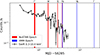 |
Fig. 1. Swift 0.3−10.0 keV light curve of AT2018cow. The times of the NuSTAR and XMM-Newton observations are highlighted with red and blue vertical lines, respectively. The six epochs we use to group the observations and the joint analysis in this paper are marked at the top of the figure. See Table B.1 for details of the observations in each epoch. We note that, at E4, the NuSTAR and XMM-Newton observations do not overlap in time. |
4. Results
Fig. 1 shows the Swift 0.3−10.0 keV light curve as well as the epochs of NuSTAR and XMM-Newton observations. We first explored the spectral characteristics by fitting the data with a fit function comprised of a power law modified by the effects of Galactic extinction (the fit function in XSPEC’s syntax is “constant*TBabs*powerlaw”). Results show that, except for Epoch 1, spectra from the other epochs can be fitted well by a power law (C-stat/d.o.f. < 2; Table B.2). From Epoch 2 to 6, the source becomes increasingly softer in X-rays, with the power–law index changing from Γ = 1.38 ± 0.02 (Epoch 2) to 2.8 ± 0.6 (Epoch 6). The soft source spectrum at the latter epoch might indicate the appearance of a soft disk component in the energy range 0.3−1.5 keV.
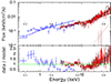 |
Fig. 2. X-ray spectra from Epoch 1 fitted by a power–law model. In the upper panel we present the data, the power–law model (solid lines), and the background models (dotted lines). The blue, black, and red data are from Swift/XRT, NuSTAR/FPMA, and NuSTAR/FPMB, respectively. In the lower panel, we show the ratio between the observed number of counts (data) and the predicted number of counts in each spectral bin (model). Similarly to what previous studies find, we observe X-ray features around ∼6.4 keV and above 10 keV that are likely due to reflection. |
From the fit residuals for Epoch 1 (Fig. 2), we confirm the X-ray features of ∼6.4 keV and ≳10 keV found previously (Margutti et al. 2019). These features cause the source spectrum to be inconsistent with a single power–law fit function at Epoch 1, and they have been proposed to be due to the reflection of the primary power–law emission (possibly caused by a BH corona or a jet base) off an accretion disk.
We then used the model relxillCp (Dauser et al. 2014; García et al. 2014; see also the References for a detailed description of each model parameter) to account for the disk reflection in the fit function. We note, in relxillCp, that the disk is assumed to be a standard Shakura–Sunyaev thin disk (Shakura & Sunyaev 1973), and the incident power–law emission is modeled by nthcomp (Zdziarski et al. 1996), which assumes a multi–temperature black body seed spectrum modified by a Comptonizing medium. Currently, there are no reflection models that use a slim disk for the disk seed photons or calculating the relativistic effect, and so we used relxillCp to approximate the reflected emission off a slim disk (the total fit function in XSPEC’s syntax is “constant*TBabs*relxillCp”). Therefore, we exercise caution when interpreting the results from our fits with relxillCp. At Epoch 1, we find the source emission is consistent with relxillCp, that is, an incident power–law–like emission plus a disk reflection (Table B.3). The Comptonizing medium is constrained, so it emits a hard power law (Γ = 1.22 ± 0.02), and its electron temperature is constrained to be 28 ± 8 keV. The inclination constraint is 74° ±2, and the BH spin constraint is 0.98 ± 0.01.
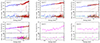 |
Fig. 3. Best–fit results based on the spectral analysis presented in Table B.3. For each figure, in the upper panel we present the spectrum and the best–fit models, and in the lower panel we present the ratio between the observed number of counts (data) and the best–fit predicted number of counts in each spectral bin (model). In all figures, the solid, dashed, dot–dashed, and dotted lines represent the best–fit source+background model, the power–law spectral component, the slim-disk component, and the background models, respectively; the blue, black, red, and magenta data are from Swift/XRT, NuSTAR/FPMA, NuSTAR/FPMB, and XMM-Newton/EPIC-pn, respectively. The y-axes in the upper panels have different scales in each figure. |
We then tested for the presence of a spectral component originating from an accretion disk in the other epochs of AT2018cow, using slimdz. The results are summarized in Table B.3. For Epochs 2 to 6, we find that it is only for Epoch 4 that the fit to the data is significantly improved by adding a disk component to the fit function (the total fit function in XSPEC’s syntax is “constant*TBabs*(powerlaw+slimdz)”; ΔAIC = 12.8; as a comparison, the power–law–only case exceeds the very strong improvement threshold of 10; Akaike 1974); statistically, Epochs 2, 3, 5, and 6 require no disk components besides a simple power law to attain a good fit to the data. Meanwhile, for Epochs 2, 3, and 5, a slim disk alone (“constant*TBabs*slimdz” in XSPEC’s syntax) cannot describe the data well. However, as the source becomes much softer at Epoch 6, we tested and find that the source spectrum at this epoch is consistent with the slim-disk model, yielding a BH mass log(M•/M⊙) = 2.3 ± 0.9, while due to data quality, other disk parameters are not well constrained (ṁ, θ, a•). The constraints on the BH mass derived from the spectra at both Epoch 4 and Epoch 6 are consistent with log(M•/M⊙)≈2.4.
Physically, it is likely that the accretion disk is present around the BH not only at Epochs 1, 4, and 6, but also throughout the period (weeks) after the first detection (Epoch 1). At Epochs 2 and 3, the soft X-ray band (0.3–3.0 keV) can only be investigated through the Swift/XRT data. As the slim disk primarily emits soft X–rays, a lack of higher-quality data in the soft band, together with the presence of a strong power–law emission component, make it impossible to constrain the disk emission at Epochs 2 and 3. At Epoch 4, however, the high-quality 0.3–3.0 keV XMM-Newton data allow significant measurements of this soft disk component to be made. At Epoch 5, the general decrease in the source luminosity makes it impossible to detect the disk in the XMM-Newton observation, especially as the source spectrum remains dominated by a power law. At Epoch 6, although the luminosity keeps decreasing, we find the source spectrum has become much softer (Table B.2). It is likely that at this epoch the luminosity of the nonthermal component has diminished and the spectrum can be explained solely by the disk emission. The disk model fits the data well without the need for nonthermal components (Fig. 3).
Therefore, based on the results above, we assumed the disk is present at all epochs and performed joint fits combining the data from Epochs 2 to 6. The total fit function in XSPEC’s syntax is “constant*TBabs*(powerlaw+slimdz)”. We forced the disk parameters θ, M•, and a• to be the same across epochs and fit their values, while we allowed ṁ to vary between epochs and treated each ṁ as an individual fit parameter for each epoch. The power–law emission was also allowed to vary between epochs in our joint fit. By jointly fitting Epochs 2 to 6, we find the BH mass to be log( , an upper limit to the inclination θ < 76°, and a broadly constrained BH spin
  . We present the full list of parameter constraints from the joint fit in Table B.4, and the ΔC-stat contour in {M•, a•} space in Fig. 4.
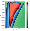 |
Fig. 4. Constraints on M• and a• based on a joint fit of the X-ray spectra from Epochs 2 to 6 with the slim-disk model (Table B.4). We calculate the ΔC-stat across the {M•, a•} plane. The best–fit point with the lowest C-stat is marked by the yellow triangle. Areas within 1σ and 2σ confidence levels are in red and blue, respectively. At 1σ for the two–parameter fits, M• is constrained to be log( |

The data at Epochs 4 and 6 play a vital role in constraining the value of the BH mass. Nonetheless, it is important that we also consider the data at other epochs, because they will help us constrain parameters that might vary over the event and can help us exclude models that are not consistent with the data (e.g., upper limits on the disk luminosity can be derived). Notably, the inclination constraint derived from the thin–disk reflection model at Epoch 1 does not deviate from the slim-disk results based on this joint fit, while the thin–disk reflection model suggests a higher BH spin than the slim-disk results. The ṁ constraints are consistent with a scenario in which the accretion rate decreases from super–Eddington to sub–Eddington levels.
In all the fits above, we notice that the re–normalization constant for the Swift spectrum at Epoch 3 is constrained to be ∼0.5, which stands out from the re–normalization of Swift observations at other epochs. We manually checked the CCD image for this particular Swift observation and find a stripe of dead pixels in the source extraction region. We also checked the other Swift data and find this row of dead pixels to be outside the source extraction region. This defect on the CCD leads to a loss in the effective instrumental area and thus results in a decrease in the number of counts in this particular spectrum, which explains the lower constant in the joint fit of the Swift spectra with those of the other satellite data.
5. Discussion
By analyzing AT2018cow data from Swift, NuSTAR, and XMM-Newton, we find that starting from Epoch 2 the source’s X-ray spectrum can be interpreted as originating from a slim disk plus a nonthermal spectral component modeled by a power law. For the X-ray spectral fits, we extended the BH mass range available for the slim-disk model slimdz (Wen et al. 2022) from 103 − 106 M⊙ to the BH mass range 101 − 106 M⊙. This extension to the model slimdz is now publicly available2 for use in XSPEC. We confirm that AT2018cow’s X-ray spectrum during Epoch 1 can be described well by a disk reflection model, as was reported before (Margutti et al. 2019). When the source becomes softer in X–rays after ≳200 days, the source spectrum becomes consistent with the emission from a slim disk. From slim-disk modeling, an IMBH of mass log( (at the 68% confidence level) is derived for the mass of the central compact object, while the disk inclination (θ < 76°) and the BH spin (
 ) are less strongly constrained (see Table B.4 for all the parameter constraints). All the parameter constraints are derived under the assumption that the disk viscosity parameter α = 0.1. Our spectral modeling shows that the X-ray spectrum becomes softer at late times due to the disappearance of the nonthermal spectral component together with a decrease in the mass accretion rate, ṁ. The ṁ values derived from our spectral fit are consistent with a decrease from super– to sub–Eddington levels at late times.
Our independent mass measurement of AT2018cow is consistent with several mass constraints available in the literature based on energetic arguments, late–time UV data modeling, and X-ray timing assumptions (Pasham et al. 2022; Migliori et al. 2023; Inkenhaag et al. 2023). The mass constraint log( confirms the presence of an accreting IMBH as the central compact object. Such an IMBH can be formed through the accretion of gas onto a seed stellar–mass BH (which can take cosmic timescales; e.g., Madau & Rees 2001; Greif et al. 2011), through the direct collapse of pristine gas clouds in the early Universe (e.g., Loeb & Rasio 1994; Bromm & Loeb 2003; Lodato & Natarajan 2006), or through BH merger events (e.g., Abbott et al. 2016). The direct mass measurement from slim-disk modeling demonstrates a possible new way to study other AT2018cow–like LFBOTs that are also accompanied by variable X-ray emission (e.g., AT2020xnd/ZTF20acigmel, Ho et al. 2022b; Bright et al. 2022; AT2020rmf, Yao et al. 2022).
An IMBH nature for AT2018cow is in line with scenarios that involve an accreting central compact object (e.g., TDE; Kuin et al. 2019; Perley et al. 2019; BH–star binary merger; Metzger 2022). In particular, for the IMBH–TDE scenario, we estimate the late–time disk outer radius to be ≈13 R⊙ given an IMBH of mass 102.4 ≈ 250 M⊙ disrupting a solar–mass star3. Thus, the predicted radius from the IMBH–TDE scenario is similar to that from the binary merger scenario (15−40 R⊙; Migliori et al. 2023) and has the same order of magnitude as values derived from the late–time UV observations (≈40 R⊙; Inkenhaag et al. 2023; Migliori et al. 2023). Meanwhile, in the core–collapse scenario, the fall–back stellar ejecta typically form a much smaller disk, and this generally leads to an outer disk radius of ∼10−3 R⊙ at late times (Migliori et al. 2023). Besides the outer disk radius, other parameters might also differ between scenarios, for example the peak ṁ. We refer to previous studies for a quantitative discussion of how those parameters depend on the BH mass in different scenarios (e.g., Metzger 2022; Migliori et al. 2023).
In our study, the nonthermal spectral component is modeled by a power–law component. Possible origins of the power–law component include a Comptonizing medium (BH corona) up–scattering the disk photons, similar to that found in other BH accretion systems like X-ray binaries or active galactic nuclei (e.g., Esin et al. 1997; Nowak et al. 2011). It is also possible that some of the nonthermal emission is generated by shock interactions with the CSM (e.g., Rivera Sandoval et al. 2018; Margutti et al. 2019; Fox & Smith 2019; Leung et al. 2020). Interestingly, when the accretion rate becomes sub–Eddington at late times, we find that the nonthermal emission diminishes and the X-ray spectrum can be fit well by a slim-disk model. Spectral state transitions involving a varying nonthermal spectral component have also been observed in several TDE systems (e.g., Bade et al. 1996; Komossa et al. 2004; Wevers et al. 2019, 2021; Jonker et al. 2020; Cao et al. 2023).
In AT2018cow, there is evidence for a dense CSM (Ho et al. 2019). Theoretical work shows that a dense CSM can be present in both a TDE scenario (Linial & Quataert 2024), where the dense CSM is produced by the outflows from the BH–star mass transfer prior to full stellar disruption, and in a binary merger scenario, where the dense CSM is produced in the common envelope phase between a stellar–mass BH (1−20 M⊙) and its massive stellar companion (Metzger 2022). At present, it is unclear if this latter model can be extrapolated to accommodate a BH of ≈250 M⊙, the value suggested by our work. If that extrapolation is plausible, our BH mass determination of AT2018cow is consistent with both the TDE and BH–star merger scenarios.
Since no reflection models for the reflected emission from a slim disk are available, in our analysis, the reflection features (i.e., the broadened iron Kα line ∼6.4 keV and the Compton hump > 10 keV) dominating the first NuSTAR epoch (and not detected in any later epochs) were modeled by disk reflection relxillCp (Dauser et al. 2014; García et al. 2014). The model relxillCp assumes that a standard thin disk reflects the emission from a Comptonizing medium with an incident power–law spectral shape. Given the same Comptonizing medium, the geometrical differences between the thin and the slim disks will result in differences in the emissivity profile of the reflected emission. This inconsistency between the likely super–Eddington accretion and the thin–disk assumption at Epoch 1 might contribute to the different spin constraints derived from the thin–disk (a• = 0.98 ± 0.01) and the slim-disk ( ) results. Despite that, we notice that the inclination constraint from relxillCp (θ = 74° ±2) is in general agreement with the value derived from the slim-disk modeling using data from all later epochs (< 76°). The material that is responsible for the reflected emission can involve the rapidly expanding outflow. Its density will decrease with time, which leads to the diminishing of reflection features in later epochs (e.g., Margutti et al. 2019).
While we extended the precalculated library of the disk spectra in slimdz to model the disk of M• < 1000 M⊙, there exists a slim-disk model slimbh (Sądowski et al. 2011; Straub et al. 2011) that is available for the disk luminosity Ldisk ≤ 1.25 LEdd (with Ldisk as one of the fit parameters in slimbh, and LEdd ≡ 1.26 × 1038(M/M⊙) erg/s)4. Physically, compared to slimbh, the slimdz model includes the loss of angular momentum due to radiation at each disk annulus. This adjustment alters the predicted effective temperature of the inner disk region, especially for high-spin, low-accretion disks (Wen et al. 2021). Moreover, a different estimate of the disk spectral hardening factor, fc (Davis & El-Abd 2019) is employed by slimdz compared with slimbh.
We compared the results derived using slimdz with those obtained using slimbh by jointly fitting Epochs 2 to 6 with the fit function “constant*TBabs*(powerlaw+slimbh)”, and comparing the results (presented in Table B.5) to the those obtained with slimdz (Table B.4). Both disk models provide a good fit to the combined data from Epochs 2 to 6. The mass constraint derived from slimbh is slightly higher (log(M•/M⊙) = 3.2 ± 0.2) though marginally consistent with that in the slimdz case (log( ). Besides the physical differences between the disk models, it is possible that when fitting the super–Eddington spectra at Epoch 4, the upper parameter range of Ldisk/LEdd ≤ 1.25 in slimbh limits the lower boundary of the mass constraint (since for a given observed luminosity, Ldisk/LEdd ∝ 1/M•). In this sense, as Ldisk/LEdd at Epoch 4 is constrained to be > 1.0 and is limited by the parameter range of ≤1.25, the lower boundary of the mass constraint derived from slimbh is underestimated, causing the mass constraints between the two disk models to be only marginally consistent in Tables B.4 and B.5. Indeed, the mass constraints derived from the two disk models are consistent when jointly fitting Epochs 5 and 6 (Table B.6), the disk likely being at sub–Eddington accretion levels at these two epochs. We also tested the α = 0.01 cases in the slimbh model. The fit results with α = 0.01 do not differ from those with α = 0.1 shown in Tables B.5 and B.6 (for slimbh cases). This test suggests that the choice of α = 0.1 does not significantly affect the slim-disk spectrum or the BH mass constraint, though the spectral library for slimdz does not currently extend to lower α values. For the above reason concerning the upper limit of Ldisk/LEdd, and due to the improved treatment of the angular momentum transport by radiation with slimdz mentioned above, we prefer the results derived from slimdz (Table B.4).
6. Conclusions
We performed X-ray spectral analysis on NuSTAR, Swift, and XMM-Newton data for the LFBOT AT2018cow and find evidence for an accretion disk soon after the source’s discovery. Based on slim-disk modeling, we constrain the mass of the central compact object to be log( at the 68% confidence level. Our mass measurement is independent from, but consistent with, the results from previously employed methods. Therefore, we provide further evidence for an accreting IMBH (102 − 106 M⊙) as the central compact object residing in AT2018cow, and by extension in similar LFBOT sources. The mass constraint is consistent with both the tidal disruption and the BH–star merger scenarios, if the latter model can be extrapolated to the measured BH mass.
Our results are consistent with the scenario in which the source accretion rate decreases from super–Eddington to sub–Eddington levels ∼200 days after its discovery. We find the late–time spectrum to be softer than the early–time spectra, which is consistent with emission from a slim disk at sub–Eddington accretion levels. In our analysis, a modified version of the existing slim-disk model slimdz is used to model the high–Eddington or super–Eddington disk of a BH at mass scales of 10 to 1000 M⊙. Through this work, we demonstrate a possible new way of studying LFBOT sources that have X-ray emissions similar to AT2018cow.
Data availability
All the X-ray data in this paper are publicly available from the HEASARC data archive (https://heasarc.gsfc.nasa.gov/). A reproduction package is available at https://doi.org/10.5281/zenodo.11110331. The extension to the slimdz model used in this paper is available at https://doi.org/10.5281/zenodo.11110331
While the slimdz model limits the disk outer radius to ≤800 Rg (for ray-tracing purposes; see Sect. 3), in the case of AT2018cow, we estimate an error on the flux of ≲0.5% introduced to the model below 1 keV by this choice of disk radius (Fig. A.1c). Meanwhile, the actual disk radius is estimated by assuming a typical TDE disk, whose outer radius is about twice the tidal radius: Rout ≈ 2 Rt = 2 Rstar(M•/Mstar)1/3 (e.g., Rees 1988; Kochanek 1994). See also the appendix.

Acknowledgments
We thank the referee for comments that helped to improve this manuscript. This work used the Dutch national e-infrastructure with the support of the SURF Cooperative using grant no. EINF-3954. This work made use of data supplied by the UK Swift Science Data Centre at the University of Leicester. P.G.J. has received funding from the European Research Council (ERC) under the European Union’s Horizon 2020 research and innovation programme (Grant agreement No. 101095973). AIZ acknowledges support in part from grant NASA ADAP #80NSSC21K0988 and grant NSF PHY-2309135 to the Kavli Institute for Theoretical Physics (KITP).
References
- Abbott, B. P., Abbott, R., Abbott, T., et al. 2016, Phys. Rev. Lett., 116, 241102 [NASA ADS] [CrossRef] [Google Scholar]
- Abramowicz, M. A., & Fragile, P. C. 2013, Liv. Rev. Relat., 16, 1 [Google Scholar]
- Abramowicz, M., Czerny, B., Lasota, J., & Szuszkiewicz, E. 1988, ApJ, 332, 646 [NASA ADS] [CrossRef] [Google Scholar]
- Adelman-McCarthy, J. K., Agüeros, M. A., Allam, S. S., et al. 2008, ApJS, 175, 297 [NASA ADS] [CrossRef] [Google Scholar]
- Akaike, H. 1974, IEEE Trans. Autom. Control, 19, 716 [Google Scholar]
- Arcavi, I., Wolf, W. M., Howell, D. A., et al. 2016, ApJ, 819, 35 [Google Scholar]
- Arnaud, K. 1996, ASP Conf. Ser., 101, 17 [NASA ADS] [Google Scholar]
- Bade, N., Komossa, S., & Dahlem, M. 1996, A&A, 309, L35 [NASA ADS] [Google Scholar]
- Bright, J. S., Margutti, R., Matthews, D., et al. 2022, ApJ, 926, 112 [NASA ADS] [CrossRef] [Google Scholar]
- Bromm, V., & Loeb, A. 2003, ApJ, 596, 34 [Google Scholar]
- Cao, Z., Jonker, P., Wen, S., Stone, N., & Zabludoff, A. 2023, MNRAS, 519, 2375 [Google Scholar]
- Cash, W. 1979, ApJ, 228, 939 [Google Scholar]
- Coppejans, D. L., Margutti, R., Terreran, G., et al. 2020, ApJ, 895, L23 [NASA ADS] [CrossRef] [Google Scholar]
- Dauser, T., García, J., Parker, M., Fabian, A., & Wilms, J. 2014, MNRAS, 444, L100 [NASA ADS] [CrossRef] [Google Scholar]
- Davis, S. W., & El-Abd, S. 2019, ApJ, 874, 23 [NASA ADS] [CrossRef] [Google Scholar]
- Dotan, C., & Shaviv, N. J. 2011, MNRAS, 413, 1623 [NASA ADS] [CrossRef] [Google Scholar]
- Drout, M. R., Chornock, R., Soderberg, A. M., et al. 2014, ApJ, 794, 23 [Google Scholar]
- Esin, A. A., McClintock, J. E., & Narayan, R. 1997, ApJ, 489, 865 [NASA ADS] [CrossRef] [Google Scholar]
- Evans, P., Beardmore, A., Page, K., et al. 2009, MNRAS, 397, 1177 [NASA ADS] [CrossRef] [Google Scholar]
- Fox, O. D., & Smith, N. 2019, MNRAS, 488, 3772 [Google Scholar]
- García, J., Dauser, T., Lohfink, A., et al. 2014, ApJ, 782, 76 [Google Scholar]
- Gottlieb, O., Tchekhovskoy, A., & Margutti, R. 2022, MNRAS, 513, 3810 [NASA ADS] [CrossRef] [Google Scholar]
- Greif, T. H., Springel, V., White, S. D., et al. 2011, ApJ, 737, 75 [NASA ADS] [CrossRef] [Google Scholar]
- Harrison, F. A., Boggs, S., Christensen, F., et al. 2010, Proc. SPIE, 7732, 189 [Google Scholar]
- Ho, A. Y., Phinney, E. S., Ravi, V., et al. 2019, ApJ, 871, 73 [NASA ADS] [CrossRef] [Google Scholar]
- Ho, A. Y., Perley, D. A., Yao, Y., et al. 2022a, ApJ, 938, 85 [NASA ADS] [CrossRef] [Google Scholar]
- Ho, A. Y., Margalit, B., Bremer, M., et al. 2022b, ApJ, 932, 116 [NASA ADS] [CrossRef] [Google Scholar]
- Ho, A. Y., Perley, D. A., Gal-Yam, A., et al. 2023, ApJ, 949, 120 [NASA ADS] [CrossRef] [Google Scholar]
- Inkenhaag, A., Jonker, P. G., Levan, A. J., et al. 2023, MNRAS, 525, 4042 [NASA ADS] [CrossRef] [Google Scholar]
- Jonker, P., Stone, N., Generozov, A., van Velzen, S., & Metzger, B. 2020, ApJ, 889, 166 [Google Scholar]
- Kaastra, J., & Bleeker, J. 2016, A&A, 587, A151 [NASA ADS] [CrossRef] [EDP Sciences] [Google Scholar]
- Katayama, H., Takahashi, I., Ikebe, Y., Matsushita, K., & Freyberg, M. 2004, A&A, 414, 767 [NASA ADS] [CrossRef] [EDP Sciences] [Google Scholar]
- Kochanek, C. S. 1994, ApJ, 422, 508 [NASA ADS] [CrossRef] [Google Scholar]
- Komossa, S., Halpern, J., Schartel, N., et al. 2004, ApJ, 603, L17 [NASA ADS] [CrossRef] [Google Scholar]
- Kuin, N. P. M., Wu, K., Oates, S., et al. 2019, MNRAS, 487, 2505 [NASA ADS] [CrossRef] [Google Scholar]
- Leung, S.-C., Blinnikov, S., Nomoto, K., et al. 2020, ApJ, 903, 66 [NASA ADS] [CrossRef] [Google Scholar]
- Leung, S.-C., Fuller, J., & Nomoto, K. 2021, ApJ, 915, 80 [NASA ADS] [CrossRef] [Google Scholar]
- Linial, I., & Quataert, E. 2024, ArXiv e-prints [arXiv:2407.00149] [Google Scholar]
- Lodato, G., & Natarajan, P. 2006, MNRAS, 371, 1813 [NASA ADS] [CrossRef] [Google Scholar]
- Loeb, A., & Rasio, F. A. 1994, ApJ, 432, 52 [Google Scholar]
- Madau, P., & Rees, M. J. 2001, ApJ, 551, L27 [Google Scholar]
- Margutti, R., Metzger, B., Chornock, R., et al. 2019, ApJ, 872, 18 [NASA ADS] [CrossRef] [Google Scholar]
- Metzger, B. D. 2022, ApJ, 932, 84 [NASA ADS] [CrossRef] [Google Scholar]
- Migliori, G., Margutti, R., Metzger, B., et al. 2023, ApJ, accepted [arXiv:2309.15678] [Google Scholar]
- Mohan, P., An, T., & Yang, J. 2020, ApJ, 888, L24 [NASA ADS] [CrossRef] [Google Scholar]
- Mummery, A., & Balbus, S. A. 2020, MNRAS, 492, 5655 [NASA ADS] [CrossRef] [Google Scholar]
- Mummery, A., van Velzen, S., Nathan, E., et al. 2024a, MNRAS, 527, 2452 [Google Scholar]
- Mummery, A., Ingram, A., Davis, S., & Fabian, A. 2024b, MNRAS, 531, 366 [NASA ADS] [CrossRef] [Google Scholar]
- Nayana, A., & Chandra, P. 2021, ApJ, 912, L9 [NASA ADS] [CrossRef] [Google Scholar]
- Nowak, M. A., Hanke, M., Trowbridge, S. N., et al. 2011, ApJ, 728, 13 [Google Scholar]
- Pagani, C., Morris, D., Racusin, J., et al. 2007, Proc. SPIE, 6686, 80 [Google Scholar]
- Pasham, D. R., Ho, W. C., Alston, W., et al. 2022, Nat. Astron., 6, 249 [Google Scholar]
- Pellegrino, C., Howell, D., Vinkó, J., et al. 2022, ApJ, 926, 125 [NASA ADS] [CrossRef] [Google Scholar]
- Perley, D. A., Mazzali, P. A., Yan, L., et al. 2019, MNRAS, 484, 1031 [Google Scholar]
- Perley, D. A., Ho, A. Y., Yao, Y., et al. 2021, MNRAS, 508, 5138 [NASA ADS] [CrossRef] [Google Scholar]
- Prentice, S., Maguire, K., Smartt, S., et al. 2018, ApJ, 865, L3 [NASA ADS] [CrossRef] [Google Scholar]
- Psaltis, D., & Johannsen, T. 2011, ApJ, 745, 1 [NASA ADS] [Google Scholar]
- Pursiainen, M., Childress, M., Smith, M., et al. 2018, MNRAS, 481, 894 [NASA ADS] [CrossRef] [Google Scholar]
- Rees, M. J. 1988, Nature, 333, 523 [Google Scholar]
- Rest, A., Garnavich, P. M., Khatami, D., et al. 2018, Nat. Astron., 2, 307 [NASA ADS] [CrossRef] [Google Scholar]
- Rivera Sandoval, L., Maccarone, T., Corsi, A., et al. 2018, MNRAS, 480, L146 [NASA ADS] [CrossRef] [Google Scholar]
- Sądowski, A., Abramowicz, M., Bursa, M., et al. 2011, A&A, 527, A17 [NASA ADS] [CrossRef] [EDP Sciences] [Google Scholar]
- Sądowski, A., Narayan, R., Tchekhovskoy, A., et al. 2015, MNRAS, 447, 49 [CrossRef] [Google Scholar]
- Shakura, N. I., & Sunyaev, R. A. 1973, A&A, 24, 337 [NASA ADS] [Google Scholar]
- Smartt, S., Clark, P., Smith, K., et al. 2018, ATel, 11727, 1 [NASA ADS] [Google Scholar]
- Straub, O., Bursa, M., Sa, A., et al. 2011, A&A, 533, A67 [NASA ADS] [CrossRef] [EDP Sciences] [Google Scholar]
- Tampo, Y., Tanaka, M., Maeda, K., et al. 2020, ApJ, 894, 27 [Google Scholar]
- Tanaka, M., Tominaga, N., Morokuma, T., et al. 2016, ApJ, 819, 5 [NASA ADS] [CrossRef] [Google Scholar]
- van Velzen, S., Stone, N. C., Metzger, B. D., et al. 2019, ApJ, 878, 82 [NASA ADS] [CrossRef] [Google Scholar]
- Wen, S., Wang, S., & Luo, X. 2018, JCAP, 2018, 011 [CrossRef] [Google Scholar]
- Wen, S., Jonker, P. G., Stone, N. C., Zabludoff, A. I., & Psaltis, D. 2020, ApJ, 897, 80 [NASA ADS] [CrossRef] [Google Scholar]
- Wen, S., Jonker, P. G., Stone, N. C., & Zabludoff, A. I. 2021, ApJ, 918, 46 [NASA ADS] [CrossRef] [Google Scholar]
- Wen, S., Jonker, P. G., Stone, N. C., Zabludoff, A. I., & Cao, Z. 2022, ApJ, 933, 31 [NASA ADS] [CrossRef] [Google Scholar]
- Wen, S., Jonker, P. G., Stone, N. C., Van Velzen, S., & Zabludoff, A. I. 2023, MNRAS, 522, 1155 [NASA ADS] [CrossRef] [Google Scholar]
- Wevers, T., Stone, N. C., van Velzen, S., et al. 2019, MNRAS, 487, 4136 [NASA ADS] [CrossRef] [Google Scholar]
- Wevers, T., Pasham, D. R., van Velzen, S., et al. 2021, ApJ, 912, 151 [NASA ADS] [CrossRef] [Google Scholar]
- Wilms, J., Allen, A., & McCray, R. 2000, ApJ, 542, 914 [Google Scholar]
- Yao, Y., Ho, A. Y., Medvedev, P., et al. 2022, ApJ, 934, 104 [NASA ADS] [CrossRef] [Google Scholar]
- Zdziarski, A. A., Johnson, W. N., & Magdziarz, P. 1996, MNRAS, 283, 193 [NASA ADS] [CrossRef] [Google Scholar]
- Zhang, W., Shu, X., Chen, J.-H., et al. 2022, RAA, 22, 125016 [NASA ADS] [Google Scholar]
Appendix A: The effect of the choice of outer disk radius in slimdz
For a 10 M⊙ BH disrupting a solar–type star, the TDE disk radius could be well above 1 × 10⁵ Rg. However, the regions ≥103 Rg contribute little to the X–ray flux, since the disk temperature decreases with radius. It is orders of magnitude lower for ≥103 Rg compared to the innermost disk region (e.g., Straub et al. 2011; Sądowski et al. 2011). As it is too expensive computationally to ray–trace the whole disk, when constructing the spectral library for slimdz, we set a fixed value of the outer disk radius, Rout, and did not ray–trace the disk region farther than Rout. Wen et al. 2021 estimate a flux error of ≲1 % when choosing Rout = 600 Rg for a 104 M⊙ BH. Here we tested different choices of Rout when ray–tracing the slim disk around a 10 M⊙ BH.
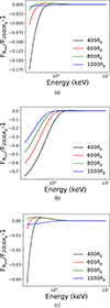 |
Fig. A.1. Effects of different choices of outer disk radius, Rout, for the ray-tracing on the emergent disk spectrum. The relative error is calculated as |
We considered a 10 M⊙ non–spinning BH with  , observed at an inclination of 45°. Figure A.1a shows the relative flux differences between different Rout choices. The relative flux error is ≲1% when Rout > 800 Rg. For higher M•, higher a•, and lower ṁ, the flux difference would be smaller, as the innermost disk region becomes more dominant than the outer disk region. Therefore, in the main text, we produce the spectral library of slimdz with Rout = 800 Rg, accelerating the calculation while the flux error is minimal.
We note that a choice of Rout = 800 Rg could introduce larger flux errors for a lower a• or for a higher ṁ. In extreme cases, for example M• = 10 M⊙, a• = −0.998, and  , the flux error could be as large as ∼50% (Fig. A.1b). Therefore, one should be cautious when modeling a retrograde stellar–mass BH and a disk of large ṁ with the currently available slimdz model.
Lastly, we estimated the flux error imposed by the choice of Rout = 800 Rg in the particular case of AT2018cow. We considered the case of M• = 250 M⊙, a• = 0.4,  , and θ = 74° (as derived from the slimdz disk modeling in Table B.4). We find a relative flux error of ≲0.5% with Rout = 800 Rg (Fig. A.1c).
Appendix B: Tables
Journal listing properties of the observations analyzed in this paper.
Parameter constraints from fitting the data within each epoch with a power–law model.
Parameter constraints from our spectral analysis, with a fit function of "constant*TBabs*relxillCp" for Epoch 1, and a fit function of "constant*TBabs*(powerlaw+slimdz)" for Epochs 2 to 6.
Same as Table B.3, but here we jointly fit all data from Epochs 2 to 6.
Same as Table B.3, but here we jointly fit all data from Epochs 2 to 6, and we replace slimdz with slimbh.
Joint fits of XMM-Newton/EPIC-pn spectra from Epochs 5 and 6.
All Tables
Parameter constraints from fitting the data within each epoch with a power–law model.
Parameter constraints from our spectral analysis, with a fit function of "constant*TBabs*relxillCp" for Epoch 1, and a fit function of "constant*TBabs*(powerlaw+slimdz)" for Epochs 2 to 6.
Same as Table B.3, but here we jointly fit all data from Epochs 2 to 6, and we replace slimdz with slimbh.
All Figures
|
Fig. 1. Swift 0.3−10.0 keV light curve of AT2018cow. The times of the NuSTAR and XMM-Newton observations are highlighted with red and blue vertical lines, respectively. The six epochs we use to group the observations and the joint analysis in this paper are marked at the top of the figure. See Table B.1 for details of the observations in each epoch. We note that, at E4, the NuSTAR and XMM-Newton observations do not overlap in time. |
| In the text | |
|
Fig. 2. X-ray spectra from Epoch 1 fitted by a power–law model. In the upper panel we present the data, the power–law model (solid lines), and the background models (dotted lines). The blue, black, and red data are from Swift/XRT, NuSTAR/FPMA, and NuSTAR/FPMB, respectively. In the lower panel, we show the ratio between the observed number of counts (data) and the predicted number of counts in each spectral bin (model). Similarly to what previous studies find, we observe X-ray features around ∼6.4 keV and above 10 keV that are likely due to reflection. |
| In the text | |
|
Fig. 3. Best–fit results based on the spectral analysis presented in Table B.3. For each figure, in the upper panel we present the spectrum and the best–fit models, and in the lower panel we present the ratio between the observed number of counts (data) and the best–fit predicted number of counts in each spectral bin (model). In all figures, the solid, dashed, dot–dashed, and dotted lines represent the best–fit source+background model, the power–law spectral component, the slim-disk component, and the background models, respectively; the blue, black, red, and magenta data are from Swift/XRT, NuSTAR/FPMA, NuSTAR/FPMB, and XMM-Newton/EPIC-pn, respectively. The y-axes in the upper panels have different scales in each figure. |
| In the text | |
|
Fig. 4. Constraints on M• and a• based on a joint fit of the X-ray spectra from Epochs 2 to 6 with the slim-disk model (Table B.4). We calculate the ΔC-stat across the {M•, a•} plane. The best–fit point with the lowest C-stat is marked by the yellow triangle. Areas within 1σ and 2σ confidence levels are in red and blue, respectively. At 1σ for the two–parameter fits, M• is constrained to be log( |
| In the text | |
|
Fig. A.1. Effects of different choices of outer disk radius, Rout, for the ray-tracing on the emergent disk spectrum. The relative error is calculated as |
| In the text | |
Current usage metrics show cumulative count of Article Views (full-text article views including HTML views, PDF and ePub downloads, according to the available data) and Abstracts Views on Vision4Press platform.
Data correspond to usage on the plateform after 2015. The current usage metrics is available 48-96 hours after online publication and is updated daily on week days.
Initial download of the metrics may take a while.