| Issue |
A&A
Volume 680, December 2023
|
|
|---|---|---|
| Article Number | A88 | |
| Number of page(s) | 9 | |
| Section | Stellar structure and evolution | |
| DOI | https://doi.org/10.1051/0004-6361/202347760 | |
| Published online | 15 December 2023 | |
NuSTAR and XMM-Newton observations of the binary 4FGL J1405.1–6119
A γ-ray-emitting microquasar?
1
Facultad de Ciencias Astronómicas y Geofísicas, Universidad Nacional de La Plata, Paseo del Bosque, B1900FWA La Plata, Argentina
e-mail: This email address is being protected from spambots. You need JavaScript enabled to view it.
2
Instituto Argentino de Radioastronomía (CCT La Plata, CONICET, CICPBA, UNLP), C.C.5, 1894 Villa Elisa, Buenos Aires, Argentina
3
Physics and Astronomy Department Galileo Galilei, University of Padova, Vicolo dell’Osservatorio 3, 35122 Padova, Italy
4
INFN – Padova, Via Marzolo 8, 35131 Padova, Italy
5
Departamento de Física (EPS), Universidad de Jaén, Campus Las Lagunillas s/n, A3, 23071 Jaén, Spain
Received:
18
August
2023
Accepted:
16
October
2023
Abstract
Context. 4FGL J1405.1−6119 is a high-mass γ-ray-emitting binary that has been studied at several wavelengths. The nature of this type of binary is still under debate, with three possible scenarios usually invoked to explain the origin of the γ-ray emission: collisions between the winds of a rapidly rotating neutron star and its companion, collisions between the winds of two massive stars, and nonthermal emission from the jet of a microquasar.
Aims. We analyzed two pairs of simultaneous NuSTAR and XMM-Newton observations to investigate the origin of the radio, X-ray, and γ-ray emissions.
Methods. We extracted light curves between 0.5 and 78 keV from two different epochs, which we call Epoch 1 and Epoch 2. We then extracted and analyzed the associated spectra to gain insight into the characteristics of the emission in each epoch. To explain these observations, along with the overall spectral energy distribution, we developed a model of a microquasar jet. This allowed us to make some inferences about the origin of the observed emission and to discuss the nature of the system.
Results. A power-law model combined with the inclusion of a blackbody accurately characterizes the X-ray spectrum. The power-law index (E−Γ) was found to be ∼1.7 for Epoch 1 and ∼1.4 for Epoch 2. Furthermore, the associated blackbody temperature was ∼1 keV and with a modeled emitting region of size ≲16 km. The scenario we propose to explain the observations involves a parabolic, mildly relativistic, lepto-hadronic jet. This jet has a compact acceleration region that injects a hard spectrum of relativistic particles. The dominant nonthermal emission processes include synchrotron radiation of electrons, inverse Compton scattering of photons from the stellar radiation field, and the decay of neutral pions resulting from inelastic proton-proton collisions within the bulk matter of the jet. These estimates are in accordance with the values of a super-Eddington lepto-hadronic jet scenario. The compact object could be either a black hole or a neutron star with a weak magnetic field. Most of the X-ray emission from the disk could be absorbed by the dense wind that is ejected from the same disk.
Conclusions. We conclude that the binary 4FGL J1405.1−6119 could be a supercritical microquasar similar to SS 433.
Key words: X-rays: binaries / gamma rays: stars
© The Authors 2023
 Open Access article, published by EDP Sciences, under the terms of the Creative Commons Attribution License (https://creativecommons.org/licenses/by/4.0), which permits unrestricted use, distribution, and reproduction in any medium, provided the original work is properly cited.
This article is published in open access under the Subscribe to Open model. This email address is being protected from spambots. You need JavaScript enabled to view it. to support open access publication.
1. Introduction
Binary sources containing neutron stars (NSs) or black holes (BHs) dominate the Galactic X-ray emission above 2 keV (see, e.g., Grimm et al. 2002). These systems are called X-ray binaries and are usually divided into two major classes, high-mass X-ray binaries and low-mass X-ray binaries, according to the mass of the donor star (mass ≳8 M⊙ for the former and ≲8 M⊙ for the latter).
Within the high-mass X-ray binary class, three types of non-transient systems can emit γ-ray radiation (Chernyakova et al. 2019; Chernyakova & Malyshev 2020):
1. Colliding-wind binaries involve the interaction of two massive stars, whose nonrelativistic winds collide and produce γ-ray emission. Prominent examples of such systems are η-Carinae, WR 11, and Apep. In colliding-wind binaries, intense shocks occur in the wind collision region, leading to the formation of a very hot plasma (> 106 K). In addition, these systems have the ability to accelerate relativistic particles (Eichler & Usov 1993; Benaglia & Romero 2003), which classifies them as particle-accelerating colliding-wind binaries (e.g., De Becker & Raucq 2013; del Palacio et al. 2023, and references therein).
2. Gamma-ray binaries are characterized by the presence of a young, magnetized, and rapidly rotating NS that emits a relativistic wind. This wind collides with the nonrelativistic wind of the companion OB star, and through this interaction they emit nonthermal radiation that peaks at high energies (E > 100 MeV). These systems are thought to represent a short phase in the evolution of massive binaries, which comes after the birth of the compact object (CO) and is followed by the X-ray binary phase, in which the CO accretes matter from its companion (e.g., Dubus et al. 2017; Saavedra et al. 2023, and references therein). In the latter phase, the nonthermal emission of the system peaks in X-rays. Examples of γ-ray binaries are LS I+61°303, PSR J1259–63, PSR J2032+4127, LS 5039, 1FGL J1018.6–5856, and HESS J0632+057.
3. Microquasars (MQs) differ from the previous two categories in that their emission of γ-rays does not come from wind collisions. Instead, it comes from the jets ejected by the CO (BH or NS) and their interaction with the environment. Examples of MQs are Cyg X-1, Cyg X-3, and SS 433.
In total, there are nine known non-transient γ-ray-emitting binaries in our Galaxy (e.g., Corbet et al. 2019; Dubus et al. 2017; Chernyakova & Malyshev 2020, and references therein). Five of these systems contain an O-type star: LS 5039, LMC P3, 1FGL J1018.6–5856, HESS J1832–093, and 4FGL J1405.1–6119. The remaining four contain a Be star: HESS J0632+057, LS I+61°303, PSR B1259–63, and PSR J2032+4127. Radio pulsations were observed in three of these systems – PSR J2032+4127 (Camilo et al. 2009), PSR B1259–63 (Moldón et al. 2014), and LS I+61°303 (Weng et al. 2022) – evidence in favor of the presence of a NS. Many more galactic γ-ray binaries are expected to exist. We recall that the nature of many of the γ-ray sources detected by telescopes such as Fermi-LAT is not known, and some of the sources may be γ-ray binaries. In fact, the number of detectable Galactic γ-ray binaries is estimated to be ∼100 (Dubus et al. 2017).
4FGL J1405.1−6119 (also known as 3FGL J1405.4−6119) is a high-mass γ-ray-emitting binary first studied by Corbet et al. (2019). Using Fermi and Swift/XRT data, Corbet et al. (2019) found a strong modulation of 13.713 ± 0.002 days associated with the system’s orbital period. The companion is classified as an O6.5 III star with a mass of about 25 − 35 M⊙ (Mahy et al. 2015). The absence of partial and total eclipses suggests that this system has a low inclination (60°).
To explain the origin of its γ-ray emission, Corbet et al. (2019) proposed that 4FGL J1405.1−6119 may be a γ-ray binary. This hypothesis draws on analogies with other similar systems, such as 1FGL J1018.6–5856 and LMC P3. Xingxing et al. (2020) modeled the GeV time behavior of 4FGL J1405.1−6119 in the γ-ray binary scenario, assuming a binary consisting of a young pulsar and an O-type main sequence star. Conversely, the radio (5.5 GHz and 9 GHz) and X-ray (0.2−10 keV) luminosities show a positive correlation (Corbet et al. 2019), as expected in MQs (Falcke et al. 2004).
We were able to perform a detailed temporal and spectral study of 4FGL J1405.1−6119 over a broad energy range by analyzing simultaneous XMM-Newton and NuSTAR observations. In this paper we present our results and conclusions about this source. In Sect. 2 we present the X-ray observations and the corresponding tools used for their analysis. Our main results are presented in Sect. 3. A jet model for the source is introduced and discussed in Sect. 4. We discuss our results and present our conclusions in Sect. 5.
2. Observation and data analysis
2.1. XMM-Newton data
The XMM-Newton observatory is equipped with an optical instrument and two X-ray instruments: the Optical Monitor, which is mounted on the mirror support platform and provides coverage between 170 nm and 650 nm of the central 17 arcmin square region; the European Photon Imaging Camera (EPIC); and the Reflecting Grating Spectrometers (RGS). The EPIC instrument comprises three detectors – the pn camera (Strüder et al. 2001) and two MOS cameras (Turner et al. 2001) – which are most sensitive in the 0.3 − 10 keV energy range. The RGS instrument comprises two high-resolution spectrographic detectors sensitive in the energy range 0.3 − 2 keV.
XMM-Newton observed 4FGL J1405.1−6119 on August 17, 2019, with an exposure time of 32 ks (ObsID 0852020101) and on August 24, 2019, with an exposure time of 44 ks (ObsID 0852020201). In both observations, the MOS cameras were in large window mode, and the pn camera was in timing mode.
We reduced the XMM-Newton data using Science Analysis System (SAS) v20.0 and the latest available calibration in early 2022. To process the observation data files, we used the EPPROC and EMPROC tasks. We selected circular regions with radii of 18 arcsec and 36 arcsec for the source and the background, respectively, with the latter away from any source contamination. We then filtered the raw events lists, removing the high-energy, single-pattern particle backgrounds and thus creating cleaned event lists for each camera and observation. The resulting exposure times after background filtering are 19 ks (59% of total) for the first observation, and 44 ks (100% of total) for the second observation. We studied the presence of pile-up with the EPATPLOT task and did not find any deviation of the data from the expected models; thus, no excision radii were applied. We barycentered each cleaned event list with the barycen task in order to perform precise timing studies. EPIC light curves were summed using the LCMATH task, with proper scaling factors for the different source photons collecting areas. We extracted and grouped spectra with a minimum of 25 counts per bin in the 0.5 − 12 keV energy band.
2.2. NuSTAR data
The NuSTAR X-ray observatory was sent into orbit in the year 2012 and is notable for its exceptional sensitivity at hard X-rays. It is equipped with two X-ray grazing incidence telescopes, designated FPMA and FPMB, which are arranged in parallel and contain 2 × 2 solid-state CdZnTe detectors each. NuSTAR can operate in the energy range of 3−79 keV and can achieve an angular resolution of 18 arcsec as reported in Harrison et al. (2013).
NuSTAR observed 4FGL J1405.1−6119 on August 16, 2019 (58711.7031 MJD – ObsID 30502015002), with an exposure of time of ∼61 ks and on August 24, 2019 (58719.3511 MJD – ObsID 30502015004) with an exposure time of ∼86 ks. We processed NuSTAR data using NuSTARDAS-v.2.1.2 from HEASoft v.6.30 and CALDB (v.20211020) calibration files. We took source events that accumulated within a circular region of 85 arcsec around the focal point. The chosen radius encloses ∼90% of the point spread function. We took a circular source-free region with a radius of 160 arcsec to obtain the background events within the same CCD.
We used the nupipeline task to create level 2 data products, with SAA parameters saacalc=1 saamode=strict tentacle=yes to filter for high-energy particle background, obtained from SAA filtering reports1. We extracted light curves and spectra with the nuproducts task. We obtained the barycenter-corrected light curves using barycorr task with nuCclock20100101v136 clock correction file. We used celestial coordinates α = 211.2472° and δ = +61.3234° for the barycentric correction with JPL-DE200 as the Solar System ephemeris. Finally, we subtracted the background from each detector’s light curve. Then we used the LCMATH task to create FPMA+B light curves. We extracted and re-binned spectra with a minimum of 25 counts per bin in the 3 − 78 keV energy band.
We used the XSPEC v12.12.1 package (Arnaud 1996) to model XMM-Newton and NuSTAR spectra, with parameters uncertainties reported at the 90% confidence level.
3. Results
3.1. Analysis of the light curves
Figure 1 shows the background-corrected light curves obtained from XMM-Newton (0.5−10 keV, top panel) and NuSTAR (3−78 keV, bottom panel) missions, with a bin time of 350 s. The observation conducted on August 17 is labeled as Epoch 1, while the observation on August 24 is labeled as Epoch 2. The long-term exposures of NuSTAR, both on the order of ∼1.5 d, show a hard X-ray flux modulation of ∼1 d seen in both epochs. The shorter but continuous exposures of XMM-Newton do not capture this behavior. Instead, it captures very short (on the order of some ks) changes in soft X-ray flux, as seen in Epoch 1.
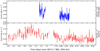 |
Fig. 1. Background-corrected light curves of 4FGL J1405.1−6119 observed by NuSTAR (FPMA+B; red) and XMM-Newton (EPIC pn+MOS; blue) with a binning of 350 s, starting at 58711.705573 MJD. The first section of the light curve corresponds to the observation from August 18 (Epoch 1), while the second light curve is associated with the observation from August 25 (Epoch 2). |
Figure 2 shows the orbital flux modulation associated with each observation and mission. Epoch 1 occurred within the orbital phases of 0.93−1.08, while Epoch 2 occurred within the orbital phases of 0.37−0.48. The observed orbital behavior of XMM-Newton and NuSTAR data is very similar to that reported by Corbet et al. (2019) using Swift/XRT data.
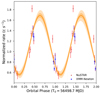 |
Fig. 2. NuSTAR and XMM-Newton folded light curve using 48 phase bins, an orbital period of 13.713 days, and with 56498.7 MJD as the reference epoch (Corbet et al. 2019). A sine function fit is shown in orange (see the main text for details). The observed orbital modulation is similar to that shown by Corbet et al. (2019) using Swift/XRT data. |
We used a sinusoidal model with Gaussian measurement errors to visualize the orbital modulation through ∼104 simulations (Buchner 2021). Specifically, the following was used:
![Mathematical equation: $$ \begin{aligned} { y} = A \,\sin \left(2\pi \left[\frac{t}{P} + t_0\right]\right) + B + \epsilon , \end{aligned} $$](/articles/aa/full_html/2023/12/aa47760-23/aa47760-23-eq1.gif) (1)
(1)
where ϵ ∼ Normal(0, σ), that is, a normal distribution with a mean of zero and a standard deviation of σ. We obtain the following values: A = 0.56 ± 0.3, P = 1.002 ± 0.002, t0 = 0.623 ± 0.001 and B = 1.13 ± 0.01. The fitted model is shown in Fig. 2.
From phase ∼0.93, the flux starts to decay, and from phase ∼0.37 the source has the maximum local emission. This modulation is anticorrelated with the modulation obtained from the Fermi data in the energy range 200 MeV−500 GeV (Corbet et al. 2019).
We employed spectral timing routines provided by Stingray software (Huppenkothen et al. 2019) to conduct a comprehensive search for any potential pulsation linked to the X-ray source. Light curves from both telescopes across various energy ranges do not show any significant pulsations above noise on the 0.1−100 mHz frequency range.
3.2. Spectral analysis
We simultaneously modeled source and background spectra extracted from all five detectors (pn, MOS1, MOS2, FPMA and FPMB). We introduced calibration constants in our models to account for disparities in effective areas between instruments. The pn constant was fixed to unity, while the remaining calibration constants were permitted to vary: CMOS1 = 1.10 ± 0.16, CMOS2 = 1.05 ± 0.15, CFPMA = 1.40 ± 0.16, and CFPMB = 1.35 ± 0.16. Each epoch was modeled separately.
The NuSTAR background showed significant activity at energies above 20 keV. As a result, we limited our analysis to the energy range 3−20 keV for both epochs. In the case of the XMM-Newton background, it was significant at energies below 2 keV. Therefore, we focused our analysis on the 2−10 keV energy range for both epochs. Consequently, the total spectrum used for each epoch included the 2−20 keV energy range.
The interstellar absorption was modeled using the Tübingen-Boulder model (tbabs), with solar abundances defined by Wilms et al. (2000) and effective cross sections of Verner et al. (1996). Several continuum models were used to fit the time-averaged spectra, including combinations of power-law variants such as powerlaw, highecut+powerlaw, cutoffpl, and bknpow, and thermal models such as apec, bbodyrad, and diskbb. After several fits, we selected the best fits: a power law (tbabs powerlaw, hereafter Model 1) and a combination of a power law and a blackbody (tbabs(powerlaw+bbodyrad), hereafter Model 2). No emission or absorption lines above the continuum were observed in the spectra of all epochs.
Model 1 yielded a χ2 of 221 with 191 degrees of freedom ( ) for Epoch 1, while Epoch 2 resulted in 184/194 − 0.95. On the other hand, if we apply Model 2, we obtain 216/189 − 1.14 for Epoch 1 and 181/192 − 0.94 for Epoch 2.
To assess the significance level of the blackbody components, we performed spectral simulations using the same observational data using FAKE-IT command from XSPEC. Each fake spectra was constructed from arrays of randomly sampled parameters using the SIMPARS command. By generating a cumulative distribution function of F-values from the simulated data, we determined the minimum significance level of detection by comparing it with the F-value derived from the real data, as described in Hurkett et al. (2008).
Each F-value, for both the real and simulated data, is calculated as  , where the subscripts 0, 1 correspond to the null hypothesis (powerlaw) and the tested hypothesis (powerlaw+bbody). Each hypothesis is associated with a total χ2 and ν degrees of freedom. The significance level is determined by computing the corresponding p value, which is the number of simulated spectra with F values greater than the F value derived from fitting the actual data. The uncertainty of this quantity can be calculated using
  , where Ns is the total number of simulated spectra.
We ran ∼105 simulations for both epochs and found that the blackbody component is significant at ∼2.6σ level for Epoch 1 and ∼2.8σ for Epoch 2.
From our analysis we conclude that the spectrum was nonthermal dominated during the observed period, possibly of synchrotron origin. This implies the presence of particles with TeV energies for the typical magnetic field strengths in this type of system. In the next section we explore this hypothesis in more detail.
In Fig. 3 we present the time averaged spectra and residuals associated with Model 1 and Model 2 of Epoch 1 (left panel) and Epoch 2 (right panel), while the corresponding best-fit parameters and uncertainties are detailed in Table 1. The powerlaw normalization component is expressed in units of photons keV−1 cm−2 s−1 at 1 keV. The bbodyrad normalization is equal to  , where Rkm is the source radius in km and D10 is the distance to the blackbody source in units of 10 kpc. At a distance of 6.7 kpc, the size of the emitting region ranged from 1.5 to 5.4 km during Epoch 1 and from 2.9 to 8.9 km during Epoch 2. Alternatively, at a distance of 8.7 kpc, the size of the emitting region ranged from 2 to 7 km for Epoch 1 and from 4 to 11.6 km for Epoch 2. In Table 1, we report the values assuming a distance of 7.7 kpc.
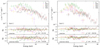 |
Fig. 3. Spectral modeling results corresponding to Epoch 1 (left column) and Epoch 2 (right column) derived from simultaneous XMM-Newton and NuSTAR data (top panels). χ2 residuals correspond to an absorbed power-law (middle panel) and absorbed power-law with a black-body component (bottom panel). |
Best-fit parameters of XMM-Newton+NuSTAR time-averaged spectral modeling of 4FGL J1405.1−6119 with const*tbabs (powerlaw) (Model 1) and const*tbabs(powerlaw+bbodyrad) (Model 2).
To compute the unabsorbed flux, we used the convolution model cflux. Assuming a distance of 7.7 kpc (Corbet et al. 2019), the unabsorbed 2−20 keV luminosity ranges between 7.2 − 7.8 × 1033 erg s−1 for Epoch 1 and 4.4 − 5 × 1033 erg s−1 for Epoch 2.
4. Model
4.1. Jet nonthermal radiation
We adopted the hypothesis that a jet is present in the γ-ray-emitting binary 4FGL J1405.1−6119, and tried to evaluate whether it can adequately explain the nonthermal spectral energy distribution (SED) of the system. The radiative jet model used follows that presented in detail in Escobar et al. (2022), which in turn is based on Romero & Vila (2008). In the following, the model setup is outlined.
The scenario consists of a CO accreting material from the companion star with an accretion power Lacc, which can be expressed in terms of the Eddington luminosity as
 (2)
(2)
where q is a constant that represents the accretion efficiency in terms of the Eddington limit. Coupled with the inner accretion disk we assume the presence of a lepto-hadronic jet of kinetic luminosity, Ljet. This jet power relates to the accretion power through
 (3)
(3)
where qjet is another constant indicating the fraction of the accretion power that is transferred to the jet. The parameters q and qjet define the accretion regime of the MQ. To compute the SED and the normalizations with the emission power, we chose to use Ljet directly as the parameter instead of a combination of q and qjet; we defer discussion of the interpretation of the accretion regime to Sect. 5.
The jet propagates with a bulk velocity vjet, corresponding to a bulk Lorentz factor Γjet. A fraction qrel of this power is converted into relativistic particles by an acceleration mechanism. The relativistic proton and electron luminosities, Lp and Le, are distributed according to the power ratio a = Lp/Le.
We use cylindrical coordinates, with the coordinate z along the jet axis and the origin at the CO. The jet is started at a distance z0 from the CO. The region in which the particles are accelerated extends from zmin to zmax, and its shape is described by
 (4)
(4)
where r0 is the radius of the jet at its base and 0 < ε ≤ 1 describes its geometry. We note that the degree of collimation of the jet increases with decreasing values of ε, with the extreme value ε = 1 representing a conical shape. The magnetic field along the jet, B, decreases with z following a power law of index m, namely, B(z) = B0(z/z0)−m, where 1 ≤ m ≤ 2 (e.g., Krolik 1999). The value of B0 is obtained by assuming equipartition between magnetic and kinetic energy at the jet base.
We parameterize the injection function of energy to relativistic particles as a power law with an exponential cutoff,
 (5)
(5)
where i = e, p accounts for electrons and protons, respectively; Qi, 0 is obtained normalizing the injection function with the total power of each particle population, Li; and Ei, max is the maximum reachable energy, achieved when the acceleration rate equals that of energy losses.
Relativistic particles are accelerated at a rate of
 (6)
(6)
where η ≤ 1 is the acceleration efficiency, c is the speed of light, and e is the elementary electric charge. On the other hand, relativistic particles lose energy via both radiative and non-radiative mechanisms. The latter are adiabatic and escape losses for both proton and electron populations. Regarding the radiative mechanisms, we consider synchrotron emission for both types of particles. In the case of protons, we also considered photons from the decay of neutral pions, which are the product of inelastic collisions between relativistic and cold protons; the latter consist mainly of protons in the jet bulk and those in the stellar wind of the companion star. In the case of electrons, we also computed the inverse Compton scattering of photons from the stellar radiation.
We assume that the relativistic particle populations reach a steady state. Their spectral densities are obtained by solving the steady state transport equation, taking injection, escape, and continuous losses into account. For a discussion of the general form of the transport equation, we refer the reader to Ginzburg & Syrovatskii (1964).
The complete formulae for calculating of radiation processes in this work can be found in Blumenthal & Gould (1970), Begelman et al. (1990), Atoyan & Dermer (2003), Kafexhiu et al. (2014), and references therein.
4.2. Spectral energy distribution of 4FGL J1405.1–6119
To fit the SED of the source with our model, we used the radio observations of Corbet et al. (2019), the X-ray flux obtained in this work, and the γ-ray flux from the 4FGL-DR2 catalog (Abdollahi et al. 2020; Ballet et al. 2020).
In Fig. 4 we show the acceleration, escape, and cooling rates of the relativistic particles at different locations in the jet. We find that for the electron population, the losses are dominated by synchrotron cooling throughout the emitting region. For the protons, both adiabatic and proton-proton collisions with bulk protons are the dominant mechanisms of energy loss in the region close to the base; the escape rate competes with them in regions further from the base and dominates the losses toward the end of the emitting region.
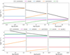 |
Fig. 4. Acceleration, escape, and cooling rates of electrons (top row) and protons (bottom row). Each column shows the aforementioned rates calculated at zmin (left column), at the logarithmic midpoint (middle column), and at zmax (right column). |
In Fig. 5 we show the derived nonthermal SED of the jet, Lγ, which includes all the above radiative processes, where
 (7)
(7)
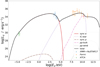 |
Fig. 5. Nonthermal SED derived from our jet model. We considered the following radiative processes: for protons, synchrotron emission and proton-proton collisions with the cold protons of the jet bulk and the companion’s wind; for electrons, synchrotron emission and inverse Compton scattering off the radiation field of the companion. The figure also shows luminosities derived from XMM-Newton+NuSTAR data (our work) as well as ATCA and Fermi data taken from Corbet et al. (2019) and the 4FGL-DR2 catalog (Abdollahi et al. 2020; Ballet et al. 2020), respectively. All the references are in the figure. |
and dN is the number of photons with energies between (Eγ, Eγ + dEγ) emitted during a time dt. The assumed and derived parameters of the model, with uncertainties reported at the 90% confidence level for the free parameters, are listed in Table 2. The X-ray data points shown in Fig. 5 correspond to Epoch 1. Since there is no significant change in the X-ray flux between the two epochs (see Fig. 1), the same set of parameters also fits the observations of Epoch 2.
Jet model parameters.
To obtain the reported model parameters, we ran a first set of ∼100 simulations2 covering a wide range of values, and decided which of these remained fixed, apart from those resulting from observed properties of the system. Then we ran another set of 120 simulations considering the variation of all free parameters (i.e., using 40 simulations for each parameter variation at a time; m, p, ε, and η), and chose the model with the minimum χ2/d.o.f. The set of values of the free parameter space was covered with a uniform grid for p, ε, m, and log η. To estimate the free parameter errors, we computed the chi-squared for each simulation and chose the  contour for each free parameter, which represents the 90% credible region (e.g., Frodesen et al. 1979). The errors are reported in Table 2. In the particular case of m (η) the upper (lower) bound on the error comes from restricting the possible values to those reported in the fourth column of Table 2, while for the case of ε all the values within the bounds fall below the aforementioned contour. We obtained a minimum chi-squared goodness of fit of χ2/d.o.f. = 1.06, with 7 d.o.f.
We show that the broad spectrum of 4FGL J1405.1−6119 can be explained by the nonthermal emission associated with a mildly relativistic (Γjet = 1.9), lepto-hadronic model of a MQ jet. In particular, this model represents an approximately parabolic jet (ε ≈ 0.56), with a compact emitting region of size ≈1.0 × 1012 cm (jet extension could be orders of magnitude larger), and a magnetic induction field at its base of B0 ≈ 2.8 × 10⁷ G. Relativistic protons and electrons share the total power in the relativistic populations, Lrel = qrelLjet = 1037 erg s−1, according to an assumed hadron-to-lepton ratio of a ≈ 0.11, and are accelerated through a low-efficiency mechanism for which η ≈ 1.0 × 10⁻⁴. The particle injection function shows a hard spectrum with spectral index p = 1.98.
In all cases, the values of the parameters are consistent with their commonly assumed range of values for MQ jets (see, for example, Romero & Vila 2008; Vila et al. 2012; Pepe et al. 2015; Escobar et al. 2021). The SED is computed assuming a viewing angle of θ = 30° (i.e., the angle between the jet axis and the line of sight). With the Lorentz factor from Table 2, and for lower viewing angles, the same data could be explained with a less powerful jet (∼0.07 times the one reported here), while higher angles would favor a scenario with more powerful jets, up to a factor of ∼50. Instead, maintaining fixed all the values of the parameters but the viewing angle, the model still manages to explain the observations with at most a variation of ≈10°. As we can see, knowing the viewing angle is a crucial factor in determining the accretion regime of the emitter.
5. Discussion and conclusions
In this work we have analyzed simultaneous XMM-Newton (2−10 keV) and NuSTAR (3−20 keV) observations of the γ-ray-emitting binary 4FGL J1405.1−6119. The difference between the two observed epochs is about six days. We found no significant pulsation above statistical noise in the XMM-Newton and NuSTAR light curves. This non-detection leaves open the question of the nature of the CO.
We fitted the time-averaged spectra of both epochs with empirical models, which yielded continuum parameters consistent with γ-ray-emitting binaries (Kretschmar et al. 2019; An et al. 2015; Yoneda et al. 2021) and MQs (Natalucci et al. 2014; Soria et al. 2020; Hirsch et al. 2020; Rodi et al. 2021; Saavedra et al. 2022). For Epoch 1, a power-law model adequately characterized the spectrum. For Epoch 2, however, the addition of a blackbody component significantly improved the fit to the observed data. The power-law index was found to be ∼1.7 for Epoch 1 and ∼1.4 for Epoch 2. Furthermore, the associated blackbody temperature for Epoch 2 was ∼0.8 keV, corresponding to a compact region of radius ≲16 km tentatively associated with the inner region of an accretion disk.
Corbet et al. (2019) present a different explanation for the emission of 4FGL J1405.1−6119. They set out a scenario involving the collision of winds between a rapidly rotating NS and its stellar companion. In addition, Xingxing et al. (2020) modeled this scenario to explain the GeV emission from 4FGL J1405.1−6119. In the colliding-wind scenario, the interaction between the stellar and pulsar winds gives rise to shocked regions that are characterized by a spiral shape due to Coriolis forces (see Molina & Bosch-Ramon 2020). Within this framework, the high-energy emission in a γ-ray binary system can be attributed to the up-scattering of photons from the stellar radiation field due to inverse Compton scattering by the relativistic electrons and positrons present in the shocked fluid. Synchrotron emission contributes to a lesser extent, especially in the energy range around ∼1 MeV (Molina & Bosch-Ramon 2020).
To explain the new X-ray data and archival multiwavelength observations (ATCA and Fermi), we implemented a lepto-hadronic jet model under the hypothesis that 4FGL J1405.1−6119 is a MQ. The parameters associated with the properties of the relativistic particle populations in the jet and the nonthermal emission are consistent with the values commonly assumed for this type of source (see, for example, Romero & Vila 2008; Vila et al. 2012; Pepe et al. 2015; Escobar et al. 2021, 2022). The scenario consists of a parabolic jet with a compact acceleration region, where the high-energy emission is produced by a hard spectrum of relativistic particles driven by a low-efficiency acceleration mechanism.
In this scenario, the γ-ray emission is produced via two processes. First, inverse Compton scattering produces nonthermal radiation in the energy range from about 100 keV to 10 GeV. Second, the decay of neutral pions from proton-proton collisions produces energetic photons at energies above 10 GeV. At lower energies, the synchrotron emission of electrons completely dominates, allowing us to accurately model radio and X-ray data. We thus propose that a lepto-hadronic jet model, which includes both leptonic and hadronic processes, may be sufficient to explain the multiwavelength emission of 4FGL J1405.1−6119.
There are essentially two interpretations of the results we obtained with our jet model. If the accretion regime is sub-Eddington, the CO should be a BH of at least ∼10 M⊙. This scenario, like the case of Cygnus X-1, would require an X-ray luminosity on the order of ∼1037 erg s−1 in the low-hard state (Di Salvo et al. 2001; Makishima et al. 2008), which is in apparent contradiction with the observations. On the other hand, if the source is in a super-Eddington accretion regime, this would imply that the CO consists of a BH of a few solar masses or a NS with a weak magnetic field. In this case, the X-ray emission from the disk is absorbed by the photosphere of the wind ejected by the same disk (Abaroa et al. 2023). This is more consistent with what is observed in the X-ray emission. The supercritical source may also have an equatorial radio component or equatorial lines with velocities of 103 − 104 km s−1, as in the case of SS 433, which could be observed in the future (Fabrika et al. 2021; Abaroa et al. 2023).
We note that leptonic jet models can also be adopted to explain observations of other MQs, as in the cases of Cyg X-3 (Zdziarski et al. 2012) and Cyg X-1 (Zdziarski et al. 2014). In our case, however, this type of model would not fully explain the observations for two main reasons. First, there is no clear evidence for disk or coronal emission. The X-ray observations could then be explained by a dominant synchrotron emission, which at these energies hides the radiation from the disk and/or the corona (see, for example, Fig. 11 of Bosch-Ramon et al. 2006). On the other hand, a relativistic proton component seems necessary to explain the observed slope change in the high-energy part of the Fermi data. In the lepto-hadronic picture, this part of the spectrum is dominated by the γ-ray emission, which originates in proton-proton collisions through neutral pion decays.
As shown in Fig. 2, the flux is higher in Epoch 1 than in Epoch 2. This behavior is also consistent with the presence of a thermal component in the spectra of Epoch 2, which can be explained by the contribution of a thermal inner disk and a reduced nonthermal jet component. In the case of a moderate or low viewing angle, some of the emission from the disk can escape from the central funnel in the wind (Abaroa et al. 2023). As for Epoch 1, the contribution to the total flux may be completely dominated by the jet.
The method we implemented for estimating parameters and uncertainties, although not very robust, allowed us to explain the multiwavelength behavior of 4FGL J1405.1−6119, favoring the MQ scenario. A more detailed analysis using a Markov chain Monte Carlo method would improve these estimates. This method would also allow a model comparison test to be included (e.g., to compute the odds ratio between leptonic and lepto-hadronic models, or between the MQ and colliding-wind scenarios). This analysis is beyond the scope of the current work, but we will present it in a future paper.
It is important to collect more observational data to evaluate the pros and cons of the pulsar-star collision wind and MQ scenarios for 4FGL J1405.1−6119. These additional data should be used to focus on timing analysis, especially with respect to the orbital period. By analyzing these data, we can gain a more complete understanding of the nature of this and other γ-ray-emitting binary systems.
We use the term “simulation” to mean the computation of the total SED with a defined set of parameters, i.e., a running of our model for a specific implementation of the parameters.
Acknowledgments
We thank the anonymous reviewer for their valuable comments on this manuscript. We extend our gratitude to Fiona A. Harrison and Brian W. Grefenstette for their assistance with the instruments’ technical aspects. We thank Sergio Campana for his suggestions that helped improve this work. E.A.S., F.A.F. and J.A.C. acknowledge support by PIP 0113 (CONICET). F.A.F. is fellow of CONICET. J.A.C. is CONICET researchers. J.A.C. is a María Zambrano researcher fellow funded by the European Union – NextGenerationEU – (UJAR02MZ). This work received financial support from PICT-2017-2865 (ANPCyT). J.A.C. was also supported by grant PID2019-105510GB-C32/AEI/10.13039/501100011033 from the Agencia Estatal de Investigación of the Spanish Ministerio de Ciencia, Innovación y Universidades, and by Consejería de Economía, Innovación, Ciencia y Empleo of Junta de Andalucía as research group FQM-322, as well as FEDER funds. G.E.R. acknowledges financial support from the State Agency for Research of the Spanish Ministry of Science and Innovation under grants PID2019-105510GB-C31AEI/10.13039/501100011033/ and PID2022-136828NB-C41/AEI/10.13039/501100011033/, and by “ERDF A way of making Europe”, by the “European Union”, and through the “Unit of Excellence María de Maeztu 2020–2023” award to the Institute of Cosmos Sciences (CEX2019-000918-M). Additional support came from PIP 0554 (CONICET). G.J.E. acknowledges financial support from the European Research Council for the ERC Consolidator grant DEMOBLACK, under contract no. 770017.
References
- Abaroa, L., Romero, G. E., & Sotomayor, P. 2023, A&A, 671, A9 [NASA ADS] [CrossRef] [EDP Sciences] [Google Scholar]
- Abdollahi, S., Acero, F., Ackermann, M., et al. 2020, ApJS, 247, 33 [Google Scholar]
- An, H., Bellm, E., Bhalerao, V., et al. 2015, ApJ, 806, 166 [NASA ADS] [CrossRef] [Google Scholar]
- Arnaud, K. A. 1996, ASP Conf. Ser., 101, 17 [Google Scholar]
- Atoyan, A. M., & Dermer, C. D. 2003, ApJ, 586, 79 [Google Scholar]
- Ballet, J., Burnett, T. H., Digel, S. W., & Lott, B. 2020, ArXiv e-prints [arXiv:2005.11208] [Google Scholar]
- Begelman, M. C., Rudak, B., & Sikora, M. 1990, ApJ, 362, 38 [Google Scholar]
- Benaglia, P., & Romero, G. E. 2003, A&A, 399, 1121 [NASA ADS] [CrossRef] [EDP Sciences] [Google Scholar]
- Blumenthal, G. R., & Gould, R. J. 1970, Rev. Mod. Phys., 42, 237 [Google Scholar]
- Bosch-Ramon, V., Romero, G. E., & Paredes, J. M. 2006, A&A, 447, 263 [NASA ADS] [CrossRef] [EDP Sciences] [Google Scholar]
- Buchner, J. 2021, J. Open Source Softw., 6, 3001 [CrossRef] [Google Scholar]
- Camilo, F., Ray, P. S., Ransom, S. M., et al. 2009, ApJ, 705, 1 [NASA ADS] [CrossRef] [Google Scholar]
- Chernyakova, M., & Malyshev, D. 2020, Multifrequency Behaviour of High Energy Cosmic Sources – XIII, 3–8 June 2019, Palermo, 45 [Google Scholar]
- Chernyakova, M., Malyshev, D., Paizis, A., et al. 2019, A&A, 631, A177 [NASA ADS] [CrossRef] [EDP Sciences] [Google Scholar]
- Corbet, R. H. D., Chomiuk, L., Coe, M. J., et al. 2019, ApJ, 884, 93 [Google Scholar]
- De Becker, M., & Raucq, F. 2013, A&A, 558, A28 [NASA ADS] [CrossRef] [EDP Sciences] [Google Scholar]
- del Palacio, S., García, F., De Becker, M., et al. 2023, A&A, 672, A109 [NASA ADS] [CrossRef] [EDP Sciences] [Google Scholar]
- Di Salvo, T., Done, C., Życki, P. T., Burderi, L., & Robba, N. R. 2001, ApJ, 547, 1024 [NASA ADS] [CrossRef] [Google Scholar]
- Dubus, G., Guillard, N., Petrucci, P.-O., & Martin, P. 2017, A&A, 608, A59 [NASA ADS] [CrossRef] [EDP Sciences] [Google Scholar]
- Eichler, D., & Usov, V. 1993, ApJ, 402, 271 [Google Scholar]
- Escobar, G. J., Pellizza, L. J., & Romero, G. E. 2021, A&A, 650, A136 [NASA ADS] [CrossRef] [EDP Sciences] [Google Scholar]
- Escobar, G. J., Pellizza, L. J., & Romero, G. E. 2022, A&A, 665, A145 [NASA ADS] [CrossRef] [EDP Sciences] [Google Scholar]
- Fabrika, S. N., Atapin, K. E., Vinokurov, A. S., & Sholukhova, O. N. 2021, Astrophys. Bull., 76, 6 [NASA ADS] [CrossRef] [Google Scholar]
- Falcke, H., Körding, E., & Markoff, S. 2004, A&A, 414, 895 [NASA ADS] [CrossRef] [EDP Sciences] [Google Scholar]
- Frodesen, A. G., Skjeggestad, O., & Tofte, H. 1979, Probability and Statistics in Particle Physics (Bergen, Norway: Universitetsforlaget) [Google Scholar]
- Ginzburg, V. L., & Syrovatskii, S. I. 1964, The Origin of Cosmic Rays (New York: Macmillan) [Google Scholar]
- Grimm, H. J., Gilfanov, M., & Sunyaev, R. 2002, A&A, 391, 923 [NASA ADS] [CrossRef] [EDP Sciences] [Google Scholar]
- Harrison, F. A., Craig, W. W., Christensen, F. E., et al. 2013, ApJ, 770, 103 [Google Scholar]
- Hirsch, M., Pottschmidt, K., Smith, D. M., et al. 2020, A&A, 636, A51 [NASA ADS] [CrossRef] [EDP Sciences] [Google Scholar]
- Huppenkothen, D., Bachetti, M., Stevens, A. L., et al. 2019, ApJ, 881, 39 [Google Scholar]
- Hurkett, C. P., Vaughan, S., Osborne, J. P., et al. 2008, ApJ, 679, 587 [NASA ADS] [CrossRef] [Google Scholar]
- Kafexhiu, E., Aharonian, F., Taylor, A. M., & Vila, G. S. 2014, Phys. Rev. D, 90, 123014 [Google Scholar]
- Kretschmar, P., Fürst, F., Sidoli, L., et al. 2019, New Astron. Rev., 86, 101546 [Google Scholar]
- Krolik, J. H. 1999, Active Galactic Nuclei: From the Central Black Hole to the Galactic Environment (Princeton: Princeton University Press) [Google Scholar]
- Mahy, L., Rauw, G., De Becker, M., Eenens, P., & Flores, C. A. 2015, A&A, 577, A23 [NASA ADS] [CrossRef] [EDP Sciences] [Google Scholar]
- Makishima, K., Takahashi, H., Yamada, S., et al. 2008, PASJ, 60, 585 [NASA ADS] [Google Scholar]
- Moldón, J., Ribó, M., Paredes, J. M., & Johnston, S. 2014, Int. J. Mod. Phys. Conf. Ser., 28, 1460173 [CrossRef] [Google Scholar]
- Molina, E., & Bosch-Ramon, V. 2020, A&A, 641, A84 [NASA ADS] [CrossRef] [EDP Sciences] [Google Scholar]
- Natalucci, L., Tomsick, J. A., Bazzano, A., et al. 2014, ApJ, 780, 63 [Google Scholar]
- Pepe, C., Vila, G. S., & Romero, G. E. 2015, A&A, 584, A95 [NASA ADS] [CrossRef] [EDP Sciences] [Google Scholar]
- Rodi, J., Tramacere, A., Onori, F., et al. 2021, ApJ, 910, 21 [NASA ADS] [CrossRef] [Google Scholar]
- Romero, G. E., & Vila, G. S. 2008, A&A, 485, 623 [NASA ADS] [CrossRef] [EDP Sciences] [Google Scholar]
- Saavedra, E. A., Sotomayor Checa, P., Vieyro, F. L., & Romero, G. E. 2022, Bol. Asoc. Argent. Astron., 63, 274 [Google Scholar]
- Saavedra, E. A., Romero, G. E., Bosch-Ramon, V., & Kefala, E. 2023, MNRAS, 525, 1848 [NASA ADS] [CrossRef] [Google Scholar]
- Soria, R., Blair, W. P., Long, K. S., Russell, T. D., & Winkler, P. F. 2020, ApJ, 888, 103 [NASA ADS] [CrossRef] [Google Scholar]
- Strüder, L., Briel, U., Dennerl, K., et al. 2001, A&A, 365, L18 [Google Scholar]
- Turner, M. J. L., Abbey, A., Arnaud, M., et al. 2001, A&A, 365, L27 [CrossRef] [EDP Sciences] [Google Scholar]
- Verner, D. A., Ferland, G. J., Korista, K. T., & Yakovlev, D. G. 1996, ApJ, 465, 487 [Google Scholar]
- Vila, G. S., Romero, G. E., & Casco, N. A. 2012, A&A, 538, A97 [NASA ADS] [CrossRef] [EDP Sciences] [Google Scholar]
- Weng, S.-S., Qian, L., Wang, B.-J., et al. 2022, Nat. Astron., 6, 698 [NASA ADS] [CrossRef] [Google Scholar]
- Wilms, J., Allen, A., & McCray, R. 2000, ApJ, 542, 914 [Google Scholar]
- Xingxing, H., Jumpei, T., & Qingwen, T. 2020, MNRAS, 494, 3699 [NASA ADS] [CrossRef] [Google Scholar]
- Yoneda, H., Khangulyan, D., Enoto, T., et al. 2021, ApJ, 917, 90 [NASA ADS] [CrossRef] [Google Scholar]
- Zdziarski, A. A., Sikora, M., Dubus, G., et al. 2012, MNRAS, 421, 2956 [NASA ADS] [CrossRef] [Google Scholar]
- Zdziarski, A. A., Pjanka, P., Sikora, M., & Stawarz, Ł. 2014, MNRAS, 442, 3243 [NASA ADS] [CrossRef] [Google Scholar]
All Tables
Best-fit parameters of XMM-Newton+NuSTAR time-averaged spectral modeling of 4FGL J1405.1−6119 with const*tbabs (powerlaw) (Model 1) and const*tbabs(powerlaw+bbodyrad) (Model 2).
All Figures
|
Fig. 1. Background-corrected light curves of 4FGL J1405.1−6119 observed by NuSTAR (FPMA+B; red) and XMM-Newton (EPIC pn+MOS; blue) with a binning of 350 s, starting at 58711.705573 MJD. The first section of the light curve corresponds to the observation from August 18 (Epoch 1), while the second light curve is associated with the observation from August 25 (Epoch 2). |
| In the text | |
|
Fig. 2. NuSTAR and XMM-Newton folded light curve using 48 phase bins, an orbital period of 13.713 days, and with 56498.7 MJD as the reference epoch (Corbet et al. 2019). A sine function fit is shown in orange (see the main text for details). The observed orbital modulation is similar to that shown by Corbet et al. (2019) using Swift/XRT data. |
| In the text | |
|
Fig. 3. Spectral modeling results corresponding to Epoch 1 (left column) and Epoch 2 (right column) derived from simultaneous XMM-Newton and NuSTAR data (top panels). χ2 residuals correspond to an absorbed power-law (middle panel) and absorbed power-law with a black-body component (bottom panel). |
| In the text | |
|
Fig. 4. Acceleration, escape, and cooling rates of electrons (top row) and protons (bottom row). Each column shows the aforementioned rates calculated at zmin (left column), at the logarithmic midpoint (middle column), and at zmax (right column). |
| In the text | |
|
Fig. 5. Nonthermal SED derived from our jet model. We considered the following radiative processes: for protons, synchrotron emission and proton-proton collisions with the cold protons of the jet bulk and the companion’s wind; for electrons, synchrotron emission and inverse Compton scattering off the radiation field of the companion. The figure also shows luminosities derived from XMM-Newton+NuSTAR data (our work) as well as ATCA and Fermi data taken from Corbet et al. (2019) and the 4FGL-DR2 catalog (Abdollahi et al. 2020; Ballet et al. 2020), respectively. All the references are in the figure. |
| In the text | |
Current usage metrics show cumulative count of Article Views (full-text article views including HTML views, PDF and ePub downloads, according to the available data) and Abstracts Views on Vision4Press platform.
Data correspond to usage on the plateform after 2015. The current usage metrics is available 48-96 hours after online publication and is updated daily on week days.
Initial download of the metrics may take a while.