| Issue |
A&A
Volume 691, November 2024
|
|
|---|---|---|
| Article Number | A320 | |
| Number of page(s) | 14 | |
| Section | Numerical methods and codes | |
| DOI | https://doi.org/10.1051/0004-6361/202451262 | |
| Published online | 22 November 2024 | |
MEGS: Morphological Evaluation of Galactic Structure
Principal component analysis as a galaxy morphology model
1
Interdisciplinary Center for Scientific Computing (IWR), University of Heidelberg,
Im Neuenheimer Feld 205,
69120
Heidelberg,
Germany
2
Universität Heidelberg, Zentrum für Astronomie, Institut für Theoretische Astrophysik,
Albert-Ueberle-Straße 2,
69120
Heidelberg,
Germany
★ Corresponding author; This email address is being protected from spambots. You need JavaScript enabled to view it.
; This email address is being protected from spambots. You need JavaScript enabled to view it.
Received:
26
June
2024
Accepted:
16
September
2024
Abstract
Context. Understanding the morphology of galaxies is a critical aspect of astrophysics research, providing insight into the formation, evolution, and physical properties of these vast cosmic structures. Various observational and computational methods have been developed to quantify galaxy morphology, and with the advent of large galaxy simulations, the need for automated and effective classification methods has become increasingly important.
Aims. This paper investigates the use of principal component analysis (PCA) as an interpretable dimensionality reduction algorithm for galaxy morphology using the IllustrisTNG cosmological simulation dataset with the aim of developing a generative model for galaxies.
Methods. We first generate a dataset of 2D images and 3D cubes of galaxies from the IllustrisTNG simulation, focusing on the mass, metallicity, and stellar age distribution of each galaxy. PCA is then applied to this data, transforming it into a lower-dimensional image space, where closeness of data points corresponds to morphological similarity.
Results. We find that PCA can effectively capture the key morphological features of galaxies, with a significant proportion of the variance in the data being explained by a small number of components. With our method we achieve a dimensionality reduction by a factor of ~200 for 2D images and ~3650 for 3D cubes at a reconstruction accuracy below 5%.
Conclusions. Our results illustrate the potential of PCA in compressing large cosmological simulations into an interpretable generative model for galaxies that can easily be used in various downstreaming tasks such as galaxy classification and analysis.
Key words: methods: statistical / techniques: image processing / astronomical databases: miscellaneous / galaxies: evolution / galaxies: kinematics and dynamics / galaxies: structure
© The Authors 2024
 Open Access article, published by EDP Sciences, under the terms of the Creative Commons Attribution License (https://creativecommons.org/licenses/by/4.0), which permits unrestricted use, distribution, and reproduction in any medium, provided the original work is properly cited.
This article is published in open access under the Subscribe to Open model. This email address is being protected from spambots. You need JavaScript enabled to view it. to support open access publication.
1 Introduction
Galaxy morphology, the study of the structural characteristics and visual appearance of galaxies, has been a significant research topic in astrophysics for many years. Early classification schemes, such as the Hubble sequence (Hubble 1926), provided a visual framework for classifying galaxies based on their visual features. Historically, galaxy morphology has also been used to identify different structural components of a galaxy through an analysis of its light profile. This process is known as structural decomposition and was first presented in an analysis by de Vaucouleurs (1958). However, these classification methods often struggled to capture the complexity and diversity of galaxy morphologies and were unable to scale with the increasing size and quality of astronomical datasets.
Fundamentally, galaxy morphology is the phenomenological realisation of the underlying fundamental differences in physical properties. The visual appearance of galaxies is heavily influenced by the joint distribution of stellar mass, metallicity, and age due to the nonlinear dependence of stellar luminosity on these fundamental parameters (e.g. Kuiper 1938). This further implies that different galaxy components trace different formation episodes of galaxies. In general, galaxy light can be modelled parametrically as either a single component (usually with a Sérsic 1963 profile), or with two or more components (e.g. Cook et al. 2019). However, in the current era of large-scale cosmological simulations, a vast amount of data are available, allowing us to investigate galaxies and their appearance in exceptional detail.
Hydrodynamical simulations of galaxy formation, such as the large-volume simulations of the IllustrisTNG suite (Pillepich et al. 2017) or the EAGLE suite (McAlpine et al. 2016) or zoom-in models such as the AURIGA (Grand et al. 2017), FIRE (Hopkins et al. 2018), VINTERGATAN (Agertz et al. 2021) or NIHAO (Wang et al. 2015; Buck et al. 2020) simulations generate rich, multidimensional datasets that include various physical properties of galaxies. These datasets provide an excellent resource for studying galaxy morphology in a more rigorous and quantitative manner. In combination with modern methods of machine learning, these simulations enable us to build an interpretable generative model for galaxy morphology (e.g. Lanusse et al. 2021).
Fast and accurate models for galaxy morphology are not only used to classify galaxies along the Hubble (1926) sequence but more recently have gained a lot of attention due to the ESA EUCLID mission. Reliable and accurate models for galaxy images are needed to achieve one of the mission’s science goals to measure the weak lensing signal (e.g. Euclid Collaboration 2022).
In this work, we set out to study principal component analysis (PCA), a relatively simple, yet powerful, and interpretable model for galaxy morphology. PCA has been widely used in various fields for dimensionality reduction and feature extraction (Jolliffe & Cadima 2016). In Turk & Pentland (1991), PCA was used to decompose face images into the subspace spanned by image eigenvectors called "eigenfaces", such that each face can be represented by a weighted sum of the eigenfaces. The term eigengalaxy first appeared in De La Calleja & Fuentes (2004), where they used PCA for galaxy classification and termed the basis vectors of the lower-dimensional space as eigengalaxies.
In the context of galaxy morphology, Uzeirbegovic et al. (2020) recently used PCA to transform a set of SDSS galaxy images into a space where ‘closeness’ corresponds to visual similarity, allowing for a quantitative measure of morphological likeliness (see also Benyas et al. 2024). Here, we expand upon their findings and explore how we can use PCA to jointly model the distribution of mass, metallicity, and stellar age in two and three dimensions. This approach specifically aims to condense a high-dimensional data distribution from galaxy simulations into a lower-dimensional space that preserves the morphological features of galaxies and allows for interpretable analysis. Our final model is able to jointly model the distribution of stellar mass, metallicity, and stellar age. In combination with a simple stellar population model to convert these parameters into stellar spectra, it is therefore ideally suited as an interpretable physics model to reconstruct the fundamental joint distribution of these properties from broad-band galaxy images.
This paper is structured as follows. In Section 2, we detail our methods. Especially, Section 2.2 discusses the methodology used for generating the dataset for our analysis by extracting galaxy data from simulations. Section 2.3 outlines the application of PCA to the image data and the resulting lower-dimensional image space (Section 2.3). Our resulting model is presented in Section 3 and its accuracy thoroughly tested in Section 3.3. In Section 3.4 we highlight potential applications of our PCA galaxy model and conclude in Section 4 with a summary and outlook of our results.
Finally, we publicly release all of our code to reproduce the results of this manuscript via GitHub1 and refer to Appendix D and Fig. C.1 for an overview of our code and file structure. Our final dataset is publicly available on Zenodo2.
2 Methods
This section outlines the methodology used to generate the dataset and build the morphology model used in this research.
2.1 Motivation
In this paper we set out to explore the possibilities of PCA to condense a high-dimensional data distribution from galaxy simulations into a lower-dimensional space that preserves key morphological features of galaxies and allows to be employed as a flexible, generative model for galaxy morphology informed by high-resolution state-of-the-art simulations. Our final method is able to project the high-dimensional joint distribution of stellar mass, metallicity, and stellar age into a lower dimensional representation which can easily be used for downstream generative modelling of galaxies. For example, in combination with a simple stellar population models to convert mass, metallic-ity and stellar age into stellar spectra, it is therefore ideally suited as an interpretable, generative physics model to reconstruct the fundamental joint distribution of these properties from broad-band galaxy images. Hence, our approach here serves the purpose of tackling the inverse problem of reconstructing physical parameters from observed data.
2.2 From simulation to dataset: galaxy image generation
We extracted galaxy data from the IllustrisTNG simulation suite (Nelson et al. 2017; Pillepich et al. 2017; Springel et al. 2017), specifically using the TNG100-1 simulation, which models galaxy formation in the cosmological context and follows 18203 resolution elements from redshift 127 to 0. From this dataset we choose snapshot number 99 since it corresponds to redshift z = 0 and extract the galaxies for our later analysis as follows:
Selection: we choose galaxies within a specified mass range of 109.5M⊙/h < M⋆ < 1013 M⊙/h, excluding galaxies with SubhaloFlag= 0, since those are not thought to be of cos-mological origin. The final selection yields a total number of N = 11960 galaxies in the dataset.
Rotation: to achieve uniform orientation and meaningful comparisons throughout the data set, we calculated the eigenvectors of the moment of inertia tensor to perform a face-on rotation in the x–y plane and obtain a set of rotated coordinates. Using these coordinates, a temporary image is generated, and a principal component analysis with two components is applied. The first principal component represents a vector that maximises the variance of the projected particle coordinates (see Uzeirbegovic et al. 2020). From this component, we determine the tilt angle and further rotate the galaxy to align its semimajor axis with the x-axis. This alignment procedure ensures consistent orientation among elliptical and barred spiral galaxies, thereby enabling reliable comparisons.
Image Rendering: to accurately capture the visual appearance of the galaxies and reflect the physical, spatial resolution of the simulation, we used the smoothing-length parameter to generate two- and three-dimensional images. Specifically, we render images in the fields of particle mass, mass-weighted metallicity, and mass-weighted stellar age3 This rendering process is performed using the render module from the SWIFTsimIO library (Borrow & Borrisov 2020). We choose an image resolution of 64 × 64 and 64 × 64 × 64 pixels for the two- and three-dimensional case, and the image section to be rendered spans five stellar half-mass radii (5Rhalf) in each direction. The resolution was chosen to correspond to the native resolution of large observational integral field spectroscopic datasets such as for example MANGA (75% of MANGA cubes have less than 64 × 64 spaxels Bundy et al. 2015) or SAMI (50x50 spaxels Allen et al. 2015) for which we have in mind that our model will be most useful.
Normalisation and Clipping: normalisation involves rescal-ing the pixel values to [0,1], which standardises the intensity levels across the images, allowing comparisons between different galaxy images. Clipping is employed to remove noise by setting a threshold for pixel values, i.e. we discard values that deviate significantly from the majority of pixels. We find that clipping values below the 25th percentile works best. This helps to highlight important features while reducing the influence of irrelevant variations which mainly arise from shot noise from the limited particle count in individual pixels originating from the limited resolution of the underlying simulations. The normalisation and clipping steps are crucial for our subsequent analysis. By eliminating noise and standardising the pixel values, we facilitate the identification and extraction of meaningful information about galaxy properties, such as morphological characteristics, stellar age distribution, and metallicity patterns. This is also needed for better PCA decomposition by removing the nuisance variance originating from random noise.
We iterate over all selected galaxies and computed both two-and three-dimensional images for the three specified fields. The resulting images are then saved in the HDF5 file format, encompassing the entire dataset. In Fig. 1 we show three representative examples of galaxies (face-on spiral, elliptical, and triaxial) in both 2D (upper panels) and 3D (lower panels). In each subfigure we show all three maps (metallicity, age, and mass from left to right). In addition to 2D images and 3D cubes, we store the SubhaloID (i.e the unique identifier of the galaxy in the simulations) and stellar mass values M⋆ for each galaxy in the attributes subgroup. It is important to note that in the case of IllustrisTNG, we exclude particles with negative GFM_StellarFormationTime, because such particles correspond to gas cells in a wind phase and are not considered relevant for the analysis. The final data set used in this work is further described in detail in Çakır & Buck (2023) and can be found publicly available here: https://github.com/ufuk-cakir/GAMMA.
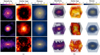 |
Fig. 1 Galaxy images (upper panels) and image cubes (lower panels) in our dataset after the preprocessing steps as explained in Section 2.2. Each row contains one sample galaxy in three stellar maps – metallicity, age and mass from left to right in (a) 2D and (b) 3D. The images are normalised in the range [0,1] and bright pixels correspond to high values. Note that in the stellar age maps, dark pixels correspond to young stars. The three dimensional plots have been created using the plotly python package. |
2.3 Principal component analysis on images
Principal component analysis (PCA) is a powerful mathematical technique commonly used in data analysis and dimensionality reduction. In simple terms, PCA finds a new set of basis vectors (principal components) that maximises the variance of the projected data in each direction. The principal components are ordered by their contribution to the total variance of the data, so the first principal component is the direction of maximal variance. Then, the dimensionality of the data space can be reduced by keeping only the top n principal components and projecting all data points onto these principal components to find a lower dimensional representation.
In the context of image analysis, PCA offers a rather simple yet powerful approach to extracting not only meaningful features from images and understanding the underlying structures in an unsupervised manner, but also to performing this in a fast and interpretable way.
In order to perform PCA, we first need to construct a proper data matrix. Each image in our dataset is represented as a two-[three-] dimensional array of size 64 × 64 [64 × 64 × 64] with values ranging from 0 to 1 . For each galaxy, the images have been calculated on three different maps (as explained in Section 2.2). These images can be reshaped into a single row vector (see Fig. 2), transforming each galaxy into a point within a high-dimensional vector space, denoted as I ∈ ℝd, where the dimensionality d is equal to the total number of pixels in the three combined maps. This results in a dimension of
 (1)
(1)
in the two and three dimensional case. Note that the order in which the three different fields are flattened is not significant as long as it remains consistent for all the galaxies. This consistency is crucial because we focus on examining the pairwise relationship between each pixel in the high-dimensional space. We finally concatenate all flattened galaxy row vectors to form our data matrix
![Mathematical equation: ${\bf{D}} = \left[ {\matrix{ {{{\bf{I}}_1}} \cr {{{\bf{I}}_2}} \cr \vdots \cr {{{\bf{I}}_N}} \cr } } \right] \in {^{N \times d}}$](/articles/aa/full_html/2024/11/aa51262-24/aa51262-24-eq2.png) (2)
(2)
with N = 11 960 (number of galaxies in the dataset) and d = d2D, d3D.
Ourgoalis to reducethe dimensionality of the original image space while retaining as much information as possible. PCA addresses this by projecting the data onto a new set of orthogonal axes that maximize the variance of the projected data. We perform PCA on our data matrix D ∈ ℝN×d using the scikit-learn (Pedregosa et al. 2011) python package. The PCA method implements the following steps in a computationally efficient way:
-
Centering: subtract the mean galaxy image to obtain the column-centered data matrix
 :
:
 (3)
(3)where µ ∈ ℝd is the column-wise mean of the data matrix D The mean images used to center the data are shown in Fig. B.1.
-
Calculate SVD: singular Value Decomposition (SVD) decomposes the centered data matrix into a product of three matrices

where U ∈ ℝN×N, V ∈ ℝd×d are unitary matrices, whose columns represent the eigenvectors of D*D*T and D*TD* respectively. The rectangular matrix Σ ∈ ℝN×d contains the singular values of D*, which are the square roots of the eigenvalues of D*TD*.
The eigenvectors correspond to the principal components of our data and are ordered by their eigenvalues, which represent the amount of variance explained by each component. The eigenvectors λ ∈ ℝd represent new orthogonal basis vectors that span our lower-dimensional image space. These eigenvectors are called eigengalaxies, since they can be interpreted as images.
We project our high-dimensional data matrix D* onto this subspace spanned by the top n eigengalaxies λn ∈ ℝn×d to obtain a lower-dimensional representation.
 (4)
(4)
where S ∈ ℝN×n contains the coordinates of N galaxy samples in the n-dimensional eigengalaxy subspace, which we also refer to as the PCA scores. This representation maintains most of the variance in the data while also reducing the dimension from d to n.
In order to transform the scores back to the original image space, we simply calculate the data matrix  containing the PCA reconstructed galaxy images as the weighted sum of n-eigengalaxies:
 (5)
(5)
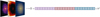 |
Fig. 2 Vectorisation in the two dimensional case: this reshaping process converts each galaxy image into a point within a high-dimensional vector space. The first 642 values correspond to the values of the pixels in the metallicity map, followed by the values of the other maps. This allows for a unique vector-based representation of each galaxy as I ∈ ℝd, where d is the dimension (Equation (1)). |
3 Results
The PCA-based morphology model provides a quantitative analysis of galaxy morphology by examining the positions of galaxies in the lower dimensional space to study morphological similarities and to model the joint distribution of mass, metallicity and stellar age. In this section we present our final PCA decomposition of galaxies in 2D and 3D and evaluate its performance via several quantitative metrics.
3.1 Dimensionality reduction and explained variance
An important quantity to evaluate how good the PCA model preserves information is the explained variance, which refers to the amount of variance of the data that is captured by each principal component, i.e., eigengalaxy. The Explained Variance Ratio (EVR) for each eigengalaxy is the proportion of the total variance of the data set that is explained by that component. Since the eigengalaxies are orthogonal, each additional eigengalaxiy accounts for variance not explained by the eigengalaxies before.
We are free to choose the total number n ofeigengalaxies we want to keep for the lower-dimensional image space representation (Section 2.3). We calculate the cumulative sum of the EVR of each eigengalaxy in Fig. 3 for up to 400 components and find that, for example 60 (215) eigengalaxies account for about 90% of the total variance in 2D (3D), which means that most of the information from the dataset can be retained even after significant dimensionality reduction (e.g. a reduction by a factor of 205 (3641)).
PCA gets better with increasing number of components, however one needs to decide for the trade-off between reconstruction accuracy and dimensionality reduction. This is showcased in Fig. 4 which contains the lower-dimensional representation of a sample galaxy (Eq. (5)) using different numbers of eigengalaxies. From top to bottom, we show the reconstructed galaxy image using 16 to 512 eigengalaxies while the bottom row shows the original image for comparison. Already with 16 eigen-galaxies the main features of the galaxy are well reconstructed, especially the spiral-like structure of stellar age. In general this figure clearly shows that with increasing number of eigengalaxies used for the reconstruction the image accuracy or the finer image details become more and more well approximated. We note that between 256 and 512 eigengalaxies we mostly observe that the noise level in the image is better approximated.
The choice of how many eigengalaxies to keep is heavily dependent on the use case, however for further analysis in this paper we use 60 (215) eigengalaxies in two (three) dimensions, since those account for 90% of explained variance as we have shown in Fig. 3. The resulting 60 eigengalaxies in the 2D case are shown in Fig. 5 and the corresponding first 60 eigengalaxies of the 3D case are shown in the appendix in Fig. D.1. We observe that the structures get much more complex as we go up to higher orders up to the scale where we observe pure rotational noise, especially visible in the case of stellar age eigenmaps. This is explained by the fact that the eigengalaxies are ordered by explained variance, and the lower orders account for more global structures. By rotational noise, we mainly refer to the fact, that galaxies show spiral arm structure and other patterns with rotational symmetry. Since PCA is a linear dimensionality reduction, it is not able to faithfully capture these features. Hence higher order eigengalaxies are needed to account for these details. This also points towards a limitation of our model and warrants to explore geometric and equivariant models in future work.
Interestingly, the physical correlation between mass, metal-licity, and age is incorporated by the fact that the stellar age eigengalaxies are almost inverted to those of metallicity and mass, since young stars have on average higher metallicity and are located in overdense regions, i.e. the spiral arms. Note that you even observe eigengalaxies with explicit spiral arms (e.g. eigengalaxy 25 in Fig. 5). Thus we conclude that decomposing the physical appearance of galaxies into eigengalaxies indeed results in an interpretable lower-dimensional representation.
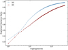 |
Fig. 3 Cumulative sum of explained variance ratio for up to 400 eigen-galaxies (left): we observe that one needs much more eigengalaxies in three dimensions to achieve the same explained variance as in two dimensions. This Figure shows that in order to achieve more than 90% EVR, you need around 60 (215) eigengalaxies in two (three) dimensions. |
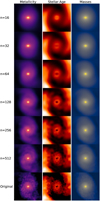 |
Fig. 4 Each column shows the lower dimensional representation using n eigengalaxies. To highlight how close we get, the original images are shown at the bottom. One can see that higher order eigengalaxies account for more detailed small scale structures, however only 16 eigen-galaxies are enough to fit the overall morphology of the galaxy. |
3.2 Reconstruction accuracy
With our final set of 60 eigengalaxies for the 2D case, we calculate the lower dimensional representation of all galaxies in our dataset. In the following we denote by Ioriginal the vector containing the pixel values of the original images and by Irec the vector containing the pixel values of the reconstructed image. In our case I ∈ ℝd is a d dimensional vector of the image space, where d is given by Eq. (1) for the 2D (3D) case. With this, we define the reconstruction error (RE) as the difference in pixel values to measure the discrepancy between the PCA representation vector Î and the original vector I
 (6)
(6)
where Îk and Ik represent the k-th elements (pixel) of the reconstructed and original vectors (images), respectively. We calculate the reconstruction error as the difference in the pixel values between the original and PCA representations separately in the three different maps. An example reconstruction for both the 2D (left panel) and 3D (right panel) case together with the residual image defined as Ioriginal − Irec is shown in Fig. 6. Qualitatively, the reconstruction in all three maps is quite well approximating the original image. We find that especially the stellar age map is approximated very well using only 60 components.
More quantitatively, we calculate the reconstruction error as defined via Eq. (6) for all galaxies in our sample and show the distribution of reconstruction errors in the top panel of Fig. 7 for both the 2D case (blue histograms) and the 3D case (red histograms). We find that 90% of all images have a reconstruction error less than 0.022 in 2D (60 eigengalaxies) and less than 0.027 in 3D (215 eigengalaxies), highlighting that our PCA model results in accurately reconstructed images.
Similarly, the bottom panel of Fig. 7 shows how the reconstruction error scales with the number of eigengalaxies used. For the 2D case we find that even with as few as ~15 eigengalax-ies 90% of all images have a reconstruction error below 0.05. In the 3D case however, we need ~60 eigengalaxies to achieve the same reconstruction error below 0.05 which is not surprising as the dimensionality of the problem is much larger. This nicely mirrors the results from the explained variance and shows that indeed only a small number of eigengalaxies are needed to accurately describe galaxy morphology.
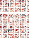 |
Fig. 5 First 60 eigengalaxies from PCA in 2D: red corresponds to high positive values, and gray corresponds to low negative values. We show the three different eigengalaxies for (a) metallicity, (b) stellar age, and (c) mass from top to bottom. |
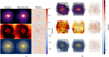 |
Fig. 6 PCA reconstruction in two and three dimensions: the left most column in each panel shows a sample galaxy in the three maps (metallicity, stellar age, and mass from top to bottom) followed by the low-dimensional PCA representation with 60 (215) eigengalaxies in a) two and b) three dimensions. The rightmost column shows the residual image (Ioriginal − Irec). You can clearly see that the complex spiral structure in the Stellar Age map is approximated very well in the two-dimensional case while at the same time at n = 60 we smooth the noise in the image. Compare also with Fig. 4 for what happens in the larger n. |
3.3 Interpretability of the model
One key advantage of PCA over more advanced machine learning methods such as neural networks is its relatively straightforward interpretability. Since PCA is a linear decomposition of the original image space, each individual component can be interpreted as an image of a very particular morphology. To visualise how eigengalaxies account for different morphology, we plot the ten eigengalaxies with the highest absolute score values used for reconstruction in Fig. A.1. We show here two example cases of the face-on spiral already shown in Fig. 4 (upper panels in Fig. A.1) and the triaxial galaxy from the bottom panels in the 2D example from Fig. 1 (lower panels in Fig. A.1).
The two columns on the left of Fig. A.1 show the original and reconstructed images, while the next ten panels show the contributing eigengalaxies in order of decreasing absolute score. The first thing to note is that vastly different eigengalaxies contribute to the reconstruction between a spiral and a triaxial galaxy (only three out of ten eigengalaxies are common, though with very different weights, compare sixth vs. third eigengalaxy in the spiral/triaxial case, which have opposite signs), as we would expect from their fundamentally different morphology. For the spiral galaxy, we find eigengalaxies with a lot of power on the diagonal edges of the image, which is needed to reconstruct the spiral arm feature. For the triaxial galaxy, on the other hand, we find that the eigengalaxies with nearly point symmetry or bar-like features contribute most to the reconstruction.
Our analysis of Fig. A.1, although quite qualitative in its nature, clearly shows the potential to describe galaxy morphology through a PCA decomposition. Fitting galaxies with our PCA model will allow one to easily study general morphological trends among different galaxies via the PCA scores of the contributing eigengalaxies (which are all the same for each galaxy by construction). For example, it is easy to select and quantify how bar-like, spiral-like, or centrally concentrated the mass, age, or metallicity distribution of a galaxy is. This further leads to one main application of describing galaxy morphology via PCA, its ability to do galaxy classification and perform a similarity search, which we describe in more depth in the next subsection.
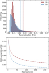 |
Fig. 7 Reconstruction Error between original images and their PCA projection. Top panel: reconstruction error for fixed dimensionality reduction onto the 60 (215) dimensional space in two (three) dimensions. The dashed line represents the 90% quantile. We observe that 90% of all images have a reconstruction error less than 0.022 (0.027). Bottom panel: 90th percentile of the reconstruction error as a function of the number of eigengalaxies used for reconstruction. The reconstruction error is a strong function of eigengalaxies, and already 15 (60) eigen-galaxies lead to a reconstruction error better than 5% in 2D (3D). |
3.4 Application
In this subsection, we highlight two potential applications of our model: (i) a similarity search among galaxies to find morphologically similar galaxies (ii) outlier detection via a UMAP projection of the PCA components.
3.4.1 Morphological similarity search
In order to test whether the lower-dimensional image space encodes morphological information, we can select a sample galaxy and search for its nearest neighbours in the PCA eigenspace using the Euclidean distance:
 (7)
(7)
where ŝ, si ∈ S (Eq. (4)) are the scores of the sample and the remaining galaxies. In Fig. A.2, we illustrate the five nearest neighbours for the two different sample galaxies already discussed in the previous Fig. A.1. Indeed, this figure shows clearly that there exists a relationship between Euclidean proximity in the PCA eigenspace and the shared morphological characteristics of galaxies. The five nearest neighbours for the spiral galaxy (left panels of Fig. A.2) all generally show a pronounced two-arm spiral galaxy where the strongest morphological similarity can be seen in the age maps (middle row). The right-hand side panels of Fig. A.2 show that indeed all neighbours of the triax-ial galaxy in the PCA eigenspace are also triaxial and share the same strong bar-like feature in mass and metallicity maps.
Similarly, the PCA scores can further be used to perform clustering analysis (e.g. using Gaussian mixture models or k-means) to define galaxy types in an unsupervised fashion or to perform an outlier detection to potentially find some interesting galaxies with morphological particularities.
3.4.2 Outlier detection
To visualise the space in two dimensions, we applied UMAP (Uniform Manifold Approximation and Projection), a dimensionality reduction and clustering algorithm developed by McInnes et al. (2020), on the lower-dimensional PCA scores. Figure A.3 shows the UMAP embedding of the PCA scores of the two-dimensional galaxy images. UMAP separates a cluster of galaxies in the dataset that deviate significantly from the rest, as shown on the left in Figure A.3. These galaxies happen to have no stars in the outer regions and therefore are reconstructed using a significantly different linear combination of eigengalaxies. By employing a threshold on the UMAP coordinates we can filter out around 120 galaxies. We rerun the analysis and fit UMAP on the PCA scores calculated on the filtered data. The resulting plot is shown on the right side of Figure A.3. The lower left quadrant of Figure A.3 mainly features spherical galaxies with little structure. In the top right section, galaxies with a prominent bar structure are aligned in a strip, whereas in the bottom right, galaxies characterized by a dominant diagonal feature form a separate cluster. Interestingly, the upper middle region of Figure A.3 is dominated by galaxies of higher mass. An interactive version of this graph can be accessed using an online dashboard4, where one can hover over each distinct point to see the corresponding galaxy image.
4 Summary and conclusions
In this study, we have explored the application of principal component analysis (PCA) to analyse galaxy images in both two-dimensional and three-dimensional cases, jointly modelling the mass, metallicity and age distributions. Our analysis has led to several findings and insights into the potential of using PCA to characterise galaxy morphology and perform morphological analysis.
We have demonstrated that PCA can be effectively used to reconstruct galaxy images using a relatively small number of eigengalaxies (Fig. 6. The reconstruction accuracy was quantified using the reconstruction error (Eq. (6)), which measures the difference in pixel values between the original and PCA-reconstructed images. Our results (Fig. 7) indicated that even with a modest number of 60 (215) eigengalaxies in 2D (3D), the PCA model achieved accurate reconstructions, with 90% of the images having reconstruction errors below 0.022 (0.027). This points to the potential of PCA for efficiently representing complex galaxy morphology.
We discussed the interpretability of the PCA model. Unlike more complex machine learning methods, PCA provides a straightforward interpretation of its components. Each eigengalaxy can be considered an image representing a specific morphological feature. Visualising the top contributing eigengalaxies for different types of galaxies revealed their distinctive contributions in Fig. A.1 and showcased the potential of PCA for classifying galaxies based on their morphology.
In terms of applications, we demonstrate the utility of PCA for performing morphological similarity searches in Fig. A.2. By measuring Euclidean distances in the PCA eigenspace, we identified morphologically similar galaxies to a given sample galaxy. This suggests that PCA captures meaningful features of galaxy morphology, allowing for efficient similarity analysis and clustering.
We showcase outlier detection using UMAP as an application of our PCA model. By inspecting a UMAP projection of the PCA scores, we are able to filter out particular galaxies that do have no stars in the outskirts.
In conclusion, this study highlights the potential of PCA as a powerful tool for analysing and characterising galaxy morphology and constructing a flexible, generative model for galaxy morphologies. Its ability to efficiently represent images, interpret its components, and facilitate morphological similarity searches makes it a valuable approach in the field of astrophysics. Our proposed PCA representation can be used to tackle the inverse problem of reconstructing physical parameters from observed data and in the case of 3D eigengalaxies it could even be used to tackle the inverse problem of deprojecting observed galaxies and reconstructing their physics parameters in 3D at the same time. Future work could involve refining the PCA model, for example using non-linear PCA, exploring its applications in other astronomical datasets, and developing hybrid approaches that combine PCA with other machine learning techniques for even more comprehensive analyses of galaxy images.
Acknowledgements
This project was made possible by funding from the Carl Zeiss Stiftung.
Appendix A Additional Figures
 |
Fig. A.1 Decomposition of two PCA reconstructed samples: The PCA reconstruction (left) is calculated as the weighted some over 60 eigengalaxies, however here we display the top 10 eigengalaxies (right), chosen based on their absolute weight values (top). On the bottom we show the corresponding index of the eigengalaxy.. This showcases the different combination of eigengalaxies used to reconstruct galaxies with different morphological features, for example spiral or bar shaped |
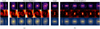 |
Fig. A.2 Nearest Neighbours in eigenspace: given a sample galaxy (left) we find the five nearest neighbours in euclidean distance in the lower dimensional space (right) for each a) spiral and b) bar shaped representative galaxy sample. |
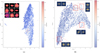 |
Fig. A.3 Outlier detection: UMAP projection with n_components=2, n_neighbors=5, min_dist=0.001 calculated (a) on the PCA components of the 2D images to find outliers (b) after filtering outlier galaxy images by choosing galaxies with UMAP1 < 2. We show some of the outliers at the top left of (a). The colour map corresponds to the masses of the galaxies in log10(M/M⊙). An interactive version of the plot on the right can be accessed using an online dashboard referenced in the GitHub repository of this work (see Appendix D) |
Appendix B Column-wise Mean of the Data Matrix
The column-wise mean of the data matrix is computed within the PCA implementation of the sklearn library. This mean is visualised in Figure B.1.
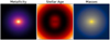 |
Fig. B.1 Columnwise mean of the Datamatrix as used in equation 3 |
Appendix C Data Structure
The dataset is stored as a HDF5 file, with the data structure shown in Figure C.1. The dataset is structured into hierarchical groups and datasets. At the top level, general galaxy parameters such as the SubhaloID from the simulation and the total stellar mass (M⋆) are stored within the /Galaxies/Attributes group. These parameters provide essential metadata for each galaxy in the simulation. Additionally, the file contains images of particle properties across different fields, including metallicity, mass, and stellar age . These images are calculated in both two and three dimensions and are saved under their respective subgroups. This structure allows for efficient access and storage of large-scale simulation data, facilitating analysis across multiple dimensions and properties.
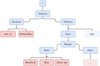 |
Fig. C.1 HDF5 File Structure, where each blue node represents a HDF5 group and red nodes are datasets. The data file contains general galaxy parameters under the /Galaxies/Attributes group such as the SubhaloID in the simulation or the total mass of stars particles M⋆. The images of particles in the different fields (i.e metallicity, mass, stellar age) are calculated in two and three dimensions and saved under the respective subgroup. |
Appendix D Code and Data Availability
The source code for the morphology model developed in this study, named MEGS, is made available under an open source license and is publicly hosted on GitHub. To facilitate a wider community’s usage and contributions, we have ensured that the repository is well-documented. The repository includes comprehensive documentation hosted on ReadThe-Docs that provides an overview of the project, installation instructions, and a guide on how to use the software.
The MEGS repository, which contains code, additional documentation, and interactive dashboards, is available on GitHub.5
The cleaned data set with outliers removed is publicly available on Zenodo.6
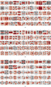 |
Fig. D.1 First 60 Eigengalaxies from PCA in 3D: For better visualization we show the images in the x-z direction, for a) Metallicity, b) Stellar Age and c) Masses. |
References
- Agertz, O., Renaud, F., Feltzing, S., et al. 2021, MNRAS, 503, 5826 [NASA ADS] [CrossRef] [Google Scholar]
- Allen, J. T., Croom, S. M., Konstantopoulos, I. S., et al. 2015, MNRAS, 446, 1567 [NASA ADS] [CrossRef] [Google Scholar]
- Benyas, M., Pfeifer, J., Mantz, A. B., Allen, S. W., & Darragh-Ford, E. 2024, ApJ, 969, 58 [NASA ADS] [CrossRef] [Google Scholar]
- Borrow, J., & Borrisov, A. 2020, J. Open Source Softw., 5, 2430 [NASA ADS] [CrossRef] [Google Scholar]
- Buck, T., Obreja, A., Macciò, A. V., et al. 2020, MNRAS, 491, 3461 [Google Scholar]
- Bundy, K., Bershady, M. A., Law, D. R., et al. 2015, ApJ, 798, 7 [Google Scholar]
- Çakir, U., & Buck, T. 2023, arXiv e-prints [arXiv:2312.06016] [Google Scholar]
- Cook, R. H. W., Cortese, L., Catinella, B., & Robotham, A. 2019, MNRAS, 490, 4060 [NASA ADS] [CrossRef] [Google Scholar]
- De La Calleja, J., & Fuentes, O. 2004, MNRAS, 349, 87 [CrossRef] [Google Scholar]
- de Vaucouleurs, G. 1958, ApJ, 128, 465 [NASA ADS] [CrossRef] [Google Scholar]
- Euclid Collaboration (Bretonnière, H., et al.) 2022, A&A, 657, A90 [CrossRef] [EDP Sciences] [Google Scholar]
- Grand, R. J. J., Gómez, F. A., Marinacci, F., et al. 2017, MNRAS, 467, 179 [NASA ADS] [Google Scholar]
- Hopkins, P. F., Wetzel, A., Kereš, D., et al. 2018, MNRAS, 480, 800 [NASA ADS] [CrossRef] [Google Scholar]
- Hubble, E. P. 1926, ApJ, 64, 321 [Google Scholar]
- Jolliffe, I. T., & Cadima, J. 2016, Philos. Trans. Roy. Soc. A: Math. Phys. Eng. Sci., 374, 20150202 [NASA ADS] [CrossRef] [Google Scholar]
- Kuiper, G. P. 1938, ApJ, 88, 472 [Google Scholar]
- Lanusse, F., Mandelbaum, R., Ravanbakhsh, S., et al. 2021, MNRAS, 504, 5543 [CrossRef] [Google Scholar]
- McAlpine, S., Helly, J., Schaller, M., et al. 2016, Astron. Comput., 15, 72 [NASA ADS] [CrossRef] [Google Scholar]
- McInnes, L., Healy, J., & Melville, J. 2020, UMAP: Uniform Manifold Approximation and Projection for Dimension Reduction [Google Scholar]
- Nelson, D., Pillepich, A., Springel, V., et al. 2017, MNRAS, 475, 624 [Google Scholar]
- Pedregosa, F., Varoquaux, G., Gramfort, A., et al. 2011, J. Mach. Learn. Res., 12, 2825 [Google Scholar]
- Pillepich, A., Nelson, D., Hernquist, L., et al. 2017, MNRAS, 475, 648 [Google Scholar]
- Sérsic, J. L. 1963, Bol. Asoc. Argentina Astron. Plata Argentina, 6, 41 [Google Scholar]
- Springel, V., Pakmor, R., Pillepich, A., et al. 2017, MNRAS, 475, 676 [Google Scholar]
- Turk, M., & Pentland, A. 1991, J. Cogn. Neurosci., 3, 71 [CrossRef] [Google Scholar]
- Uzeirbegovic, E., Geach, J. E., & Kaviraj, S. 2020, MNRAS, 498, 4021 [CrossRef] [Google Scholar]
- Wang, L., Dutton, A. A., Stinson, G. S., et al. 2015, MNRAS, 454, 83 [NASA ADS] [CrossRef] [Google Scholar]
In the IllustrisTNG catalogue these correspond to the fields: Masses, GFM_Metallicity and GFM_StellarFormationTime. Note that we convert the time the star was born to an age using the age of the universe, so low values correspond to young stars.
All Figures
|
Fig. 1 Galaxy images (upper panels) and image cubes (lower panels) in our dataset after the preprocessing steps as explained in Section 2.2. Each row contains one sample galaxy in three stellar maps – metallicity, age and mass from left to right in (a) 2D and (b) 3D. The images are normalised in the range [0,1] and bright pixels correspond to high values. Note that in the stellar age maps, dark pixels correspond to young stars. The three dimensional plots have been created using the plotly python package. |
| In the text | |
|
Fig. 2 Vectorisation in the two dimensional case: this reshaping process converts each galaxy image into a point within a high-dimensional vector space. The first 642 values correspond to the values of the pixels in the metallicity map, followed by the values of the other maps. This allows for a unique vector-based representation of each galaxy as I ∈ ℝd, where d is the dimension (Equation (1)). |
| In the text | |
|
Fig. 3 Cumulative sum of explained variance ratio for up to 400 eigen-galaxies (left): we observe that one needs much more eigengalaxies in three dimensions to achieve the same explained variance as in two dimensions. This Figure shows that in order to achieve more than 90% EVR, you need around 60 (215) eigengalaxies in two (three) dimensions. |
| In the text | |
|
Fig. 4 Each column shows the lower dimensional representation using n eigengalaxies. To highlight how close we get, the original images are shown at the bottom. One can see that higher order eigengalaxies account for more detailed small scale structures, however only 16 eigen-galaxies are enough to fit the overall morphology of the galaxy. |
| In the text | |
|
Fig. 5 First 60 eigengalaxies from PCA in 2D: red corresponds to high positive values, and gray corresponds to low negative values. We show the three different eigengalaxies for (a) metallicity, (b) stellar age, and (c) mass from top to bottom. |
| In the text | |
|
Fig. 6 PCA reconstruction in two and three dimensions: the left most column in each panel shows a sample galaxy in the three maps (metallicity, stellar age, and mass from top to bottom) followed by the low-dimensional PCA representation with 60 (215) eigengalaxies in a) two and b) three dimensions. The rightmost column shows the residual image (Ioriginal − Irec). You can clearly see that the complex spiral structure in the Stellar Age map is approximated very well in the two-dimensional case while at the same time at n = 60 we smooth the noise in the image. Compare also with Fig. 4 for what happens in the larger n. |
| In the text | |
|
Fig. 7 Reconstruction Error between original images and their PCA projection. Top panel: reconstruction error for fixed dimensionality reduction onto the 60 (215) dimensional space in two (three) dimensions. The dashed line represents the 90% quantile. We observe that 90% of all images have a reconstruction error less than 0.022 (0.027). Bottom panel: 90th percentile of the reconstruction error as a function of the number of eigengalaxies used for reconstruction. The reconstruction error is a strong function of eigengalaxies, and already 15 (60) eigen-galaxies lead to a reconstruction error better than 5% in 2D (3D). |
| In the text | |
|
Fig. A.1 Decomposition of two PCA reconstructed samples: The PCA reconstruction (left) is calculated as the weighted some over 60 eigengalaxies, however here we display the top 10 eigengalaxies (right), chosen based on their absolute weight values (top). On the bottom we show the corresponding index of the eigengalaxy.. This showcases the different combination of eigengalaxies used to reconstruct galaxies with different morphological features, for example spiral or bar shaped |
| In the text | |
|
Fig. A.2 Nearest Neighbours in eigenspace: given a sample galaxy (left) we find the five nearest neighbours in euclidean distance in the lower dimensional space (right) for each a) spiral and b) bar shaped representative galaxy sample. |
| In the text | |
|
Fig. A.3 Outlier detection: UMAP projection with n_components=2, n_neighbors=5, min_dist=0.001 calculated (a) on the PCA components of the 2D images to find outliers (b) after filtering outlier galaxy images by choosing galaxies with UMAP1 < 2. We show some of the outliers at the top left of (a). The colour map corresponds to the masses of the galaxies in log10(M/M⊙). An interactive version of the plot on the right can be accessed using an online dashboard referenced in the GitHub repository of this work (see Appendix D) |
| In the text | |
|
Fig. B.1 Columnwise mean of the Datamatrix as used in equation 3 |
| In the text | |
|
Fig. C.1 HDF5 File Structure, where each blue node represents a HDF5 group and red nodes are datasets. The data file contains general galaxy parameters under the /Galaxies/Attributes group such as the SubhaloID in the simulation or the total mass of stars particles M⋆. The images of particles in the different fields (i.e metallicity, mass, stellar age) are calculated in two and three dimensions and saved under the respective subgroup. |
| In the text | |
|
Fig. D.1 First 60 Eigengalaxies from PCA in 3D: For better visualization we show the images in the x-z direction, for a) Metallicity, b) Stellar Age and c) Masses. |
| In the text | |
Current usage metrics show cumulative count of Article Views (full-text article views including HTML views, PDF and ePub downloads, according to the available data) and Abstracts Views on Vision4Press platform.
Data correspond to usage on the plateform after 2015. The current usage metrics is available 48-96 hours after online publication and is updated daily on week days.
Initial download of the metrics may take a while.