| Issue |
A&A
Volume 669, January 2023
|
|
|---|---|---|
| Article Number | A152 | |
| Number of page(s) | 18 | |
| Section | Numerical methods and codes | |
| DOI | https://doi.org/10.1051/0004-6361/202244481 | |
| Published online | 27 January 2023 | |
Spatial field reconstruction with INLA
Application to simulated galaxies
1
Astronomical Observatory,
Volgina 7,
11060
Belgrade, Serbia
e-mail: msmole@aob.rs
2
CENTRA, Instituto Superior Técnico,
Av. Rovisco Pais,
Lisboa
1049-001, Portugal
3
Sterrenkundig Observatorium, Universiteit Gent,
Krijgslaan 281-S9,
Gent
9000, Belgium
Received:
12
July
2022
Accepted:
29
October
2022
Aims. Monte Carlo radiative transfer (MCRT) simulations are a powerful tool for understanding the role of dust in astrophysical systems and its influence on observations. However, due to the strong coupling of the radiation field and medium across the whole computational domain, the problem is non-local and non-linear, and such simulations are computationally expensive in the case of realistic 3D inhomogeneous dust distributions. We explore a novel technique for post-processing MCRT output to reduce the total computational run time by enhancing the output of computationally less expensive simulations of lower-quality.
Methods. We combined principal component analysis (PCA) and non-negative matrix factorisation (NMF) as dimensionality reduction techniques together with Gaussian Markov random fields and the integrated nested Laplace approximation (INLA), an approximate method for Bayesian inference, to detect and reconstruct the non-random spatial structure in the images of lower signal-to-noise ratios or with missing data.
Results. We tested our methodology using synthetic observations of a galaxy from the SKIRT Auriga project - a suite of high-resolution magnetohydrodynamic Milky Way-sized galaxies simulated in cosmological environment using a ‘zoom-in' technique. With this approach, we are able to reproduce high-photon-number reference images ~5 times faster with median residuals below ~20%.
Key words: galaxies: general / dust / extinction / radiative transfer / methods: numerical / techniques: image processing
© The Authors 2023
 Open Access article, published by EDP Sciences, under the terms of the Creative Commons Attribution License (https://creativecommons.org/licenses/by/4.0), which permits unrestricted use, distribution, and reproduction in any medium, provided the original work is properly cited.
This article is published in open access under the Subscribe-to-Open model. Subscribe to A&A to support open access publication.
1 Introduction
Cosmological simulations provide a powerful tool for understanding galaxy formation, their evolution, and cosmic structure on large scales. State-of-the-art hydrodynamical simulations use sub-grid physics for processes such as radiative cooling, star formation, metal enrichment, and active galactic nucleus (AGN) feedback. Examples of such hydrodynamical cosmological simulations include the Illustris (Vogelsberger et al. 2014a,b; Genel et al. 2014), EAGLE (Crain et al. 2015; Schaye et al. 2015), and IllustrisTNG projects (Weinberger et al. 2017; Pillepich et al. 2018).
Both observational and simulated data can be fully exploited only by their detailed comparison. Observations are required to test the results of numerical simulations. On the other hand, simulations can support the interpretation of observations and constrain predictions for the future instruments and observational missions. One of the challenges includes the possibility that the observed radiation may have been altered by the medium between the emitting source and the observer. Given the high abundance of dust in the interstellar medium, dust grains have considerable importance in shaping the observed signal, absorbing and scattering ultraviolet and optical radiation, and then re-emitting the absorbed energy at infrared wavelengths. Thus, the observed signal provides information about the emitting source and at the same time reveals the properties of the medium on its path.
Synthetic observations can be used to fill a gap between properties derived from numerical simulations and real observations. They are generated, for example, starting from a snapshot of an output of a hydrodynamical simulation and solving the radiative transfer (RT) problem by simulating how radiation propagates from an astrophysical source to the observer, optionally taking into account the degradation of the image due to transfer through the atmosphere and optics of the instrument. RT simulations play an important role in our understanding of the effects of dust on astrophysical observations. However, realistic dusty media are often complex and inhomogeneous, and calculating the propagation of radiation in such systems requires the implementation of special numerical methods, such as Monte Carlo radiative transfer (MCRT). These simulations use a large number of photon packages and emulate the relevant physical processes to mimic the propagation of real photons in dusty environments. We refer the reader to Steinacker et al. (2013) for a review of numerical solution techniques for 3D dust RT problems and to Noebauer & Sim (2019) for a recent review of MCRT codes.
Different studies offer publicly available synthetic observational data for cosmological simulations, using the zoom-in technique. This technique involves a process where an additional zoom-in simulation with higher mass and/or time resolution is performed for a selected part of the original simulation. Initial conditions are taken directly from a cosmological simulation, with further implementation of sub-grid physics of relevant processes that cannot be resolved directly in the simulations. Recent examples include studies by Kapoor et al. (2021) and Camps et al. (2022), which provide high-resolution broadband images of galaxies in the Auriga (Grand et al. 2017) and ARTEMIS (Font et al. 2020) projects, respectively. However, even with state-of-the-art MCRT codes, simulating high-resolution synthetic images proves to be a computationally challenging task (Steinacker et al. 2013). Memory requirements and simulation running times increase with the volume grid density and with the amount of photon packages used. In this work, our goal is to develop an MCRT post-processing methodology capable of achieving the quality of high-photon-number images using low-photon-number images as an input. We explored the potential of the integrated nested Laplace approximation (INLA, Rue et al. 2009, 2017), an approximate method for Bayesian inference, along with Gaussian Markov random fields to detect and reconstruct the non-random spatial structure of simulated galaxies. The capability of this INLA method to reveal the underlying spatial structure of astronomical data has already been tested (González-Gaitán et al. 2019). Applied to integral field unit (IFU) galaxy data, INLA is able to recover structures otherwise hidden, even with highly sparse spatial information. The INLA method has been successfully applied to various research fields; a few examples include identifying the climatic drivers of honey bee disease in England and Wales (Rowland et al. 2021), forecasting deforestation in the Brazilian Amazon (Jaffé et al. 2021), and mapping air pollution (Gong et al. 2021).
Alongside the work presented here, we developed an alternative post-processing methodology for MCRT codes, combining an auto-encoder neural network and INLA (Rino-Silvestre et al. 2022). Here, we offer another methodology combining principal component analysis (PCA) and non-negative matrix factorisation (NMF) as dimensionality reduction techniques together with INLA and test the performance using high-resolution broadband images of galaxies from the Auriga project (Grand et al. 2017).
In Sect. 2, we introduce the employed techniques and codes, together with datasets used in this work, and we describe their implementation in our methodology. We applied our method to a galaxy from the Auriga project. Results are presented and discussed in Sect. 3. In Sect. 4, we summarise the main findings of this work and draw conclusions.
2 Methods
2.1 Simulated data
2.1.1 SKIRT code
The SKIRT1 is a flexible MCRT code that can simulate the propagation of the radiation through dusty media with arbitrary 3D geometries (Baes & Camps 2015; Camps & Baes 2015). Trajectories of the photon packages, emitted by primary sources, are calculated by taking into account scattering, absorption, and thermal re-emission by dust grains. Their progress through a dusty medium is calculated statistically, generating random numbers from the appropriate probability density function for each of the relevant processes. Since the interaction of each individual photon package with the medium is obtained using probability density functions, the number of photon packages in the simulation has to be large enough to provide an accurate description of the radiation field.
The SKIRT code has been widely used to study dust properties in spiral galaxies (Baes et al. 2010; De Looze et al. 2012a,b; De Geyter et al. 2015), sub-millimetre galaxies (Dudzeviciute et al. 2020), dust-driven properties of high-redshift galaxies (Behrens et al. 2018; Vijayan et al. 2022), galaxy evolution (Whitney et al. 2021; Deeley et al. 2021; Zanella et al. 2021), dust attenuation law in high-redshift quasars (Di Mascia et al. 2021), and in investigating AGN structure (Stalevski et al. 2016, 2017, Stalevski et al. 2019), to name a few applications2.
2.1.2 Auriga galaxies
The Auriga project3 provides a set of cosmological magneto-hydrodynamical zoom-in simulations of Milky Way (MW) type galaxies (Grand et al. 2017). Simulations were performed using the hydrodynamic moving mesh code AREPO (Springel 2010), with a complete treatment of galaxy formation and evolution process such as gas cooling and heating, star formation, black hole and stellar feedback, etc. (Vogelsberger et al. 2013; Genel et al. 2014).
The SKIRT Auriga project4 offers high resolution synthetic images of 30 simulated MW type galaxies from the Auriga project (Kapoor et al. 2021). This synthetic observational data, obtained with SKIRT, represents a sample of z = 0 galaxies in the broad wavelength range from UV to sub-mm. For each galaxy, sets of star particles and gas cells are extracted from the Auriga simulation snapshots. Star particles with an age above 10Myr are assigned a spectral energy distribution (SED) using Bruzual & Charlot (2003) stellar template library, based on metallicity and age. Star particles with an age below 10Myr are assumed to be surrounded by dust in star-forming regions, and they are assigned SED from the MAPPINGS III (Groves et al. 2008) template library. The initial dust distribution is calculated based on the metallicity and gas density extracted from the Auriga snapshots, using the THEMIS dust model (Jones et al. 2017). We refer to Kapoor et al. (2021) for detailed recipes for the transformation from the set of particles extracted from Auriga snapshot to the set of particles used in SKIRT simulation.
Synthetic images from the SKIRT Auriga project are publicly available in the flexible image transport system (FITS) format composed of 2D spatial distributions at 50 different wavelength bins. Three different inclinations of the galaxy that is the angle between the angular momentum vector and the direction towards the observer comprise the dataset of each galaxy: ‘face-on’ (i = 0°), ‘edge-on’ (i = 90°) and ‘intermediate’ (i = 115°). ‘Intermediate’ viewing angle corresponds to the original orientation of the galaxy in the simulation box.
2.2 INLA
INLA (Rue et al. 2009) is a computational method for approximate Bayesian inference of latent Gaussian fields. Bayesian inference is a process of deducing a probability distribution from data using Bayes theorem. Bayesian inference (Eq. (1)) calculates a posterior distribution  , for the given model likelihood
  , prior distribution π(θ), and marginal likelihood
  :
:

Most techniques for calculating posterior distribution rely on Markov chain Monte Carlo (MCMC) methods (Collins et al. 1974). In this class of sampling-based numerical methods, the posterior distribution is obtained after many iterations, which is often computationally expensive. INLA provides a novel approach for faster Bayesian inference. While MCMC methods draw a sample from the joint posterior distribution, the Laplace approximation is a method that approximates posterior distributions of the model parameters to Gaussians, which is computationally more effective.
Within the INLA framework, the posterior distribution ofthe latent Gaussian variables x and hyperparameters of the model θ is

where y = (y1,…,yn) represents set of observations or a pixel matrix. Every pixel is treated with a latent Gaussian effect so that each xi (which is just the mean value µi and standard deviation σi of a Gaussian for a pixel yi) corresponds to observation yi, where i ∈ [1,…, n]. The observations are conditionally independent given the latent effect x and the hyperparameters θ, so the model likelihood is

The joint distribution of the latent effects and the hyperparameters, π(x, θ) can be written as  , where π(θ) represents the prior distribution of hyperparameters θ. It is assumed that the spatial information can be treated as a discrete sampling of an underlying continuous spatial field, a latent Gaussian Markov random field (GMRF), which takes into account the spatial correlations, and whose hyperparameters are inferred in the process. For a GMRF, the posterior distribution of the latent effects is
![$\pi \left( {{\bf{x}}\left| {\bf{\theta }} \right.} \right) \propto {\left| {{\bf{Q}}\left( {\bf{\theta }} \right)} \right|^{1/2}}\exp \left[ { - {1 \over 2}{{\bf{x}}^T}{\bf{Q}}\left( {\bf{\theta }} \right){\bf{x}}} \right],$](/articles/aa/full_html/2023/01/aa44481-22/aa44481-22-eq8.png)
where Q(θ) represents a precision matrix, or inverse of a covari-ance matrix, which depends on a vector of hyperparameters θ. This kernel matrix is what actually treats the spatial correlation between neighbouring pixels. Using Eq. (2), the joint posterior distribution of the latent effects and hyperparameters can be written as
![$\matrix{{\pi \left( {{\bf{x}},\left. {\bf{\theta }} \right|{\bf{y}}} \right) \propto \pi \left( {\bf{\theta }} \right){{\left| {{\bf{Q}}\left( {\bf{\theta }} \right)} \right|}^{{1 \mathord{\left/{\vphantom {1 2}} \right.\kern-\nulldelimiterspace} 2}}}\exp \left[ { - {1 \over 2}{{\bf{x}}^T}{\bf{Q}}\left( {\bf{\theta }} \right)x} \right]\prod\limits_i {\pi \left( {{y_i}\left| {{x_i},{\bf{\theta }}} \right.} \right)} } \hfill \cr {\,\,\,\,\,\, = \pi \left( {\bf{\theta }} \right){{\left| {{\bf{Q}}\left( {\bf{\theta }} \right)} \right|}^{{1 \mathord{\left/{\vphantom {1 2}} \right.\kern-\nulldelimiterspace} 2}}}\exp \left[ { - {1 \over 2}{{\bf{x}}^T}{\bf{Q}}\left( {\bf{\theta }} \right){\bf{x}} + \sum\limits_i {\log \left( {\pi \left( {\left. {{y_i}} \right|{x_i},{\bf{\theta }}} \right)} \right)} } \right].} \hfill \cr } $](/articles/aa/full_html/2023/01/aa44481-22/aa44481-22-eq9.png)
Instead of obtaining the exact posterior distribution from Eq. (5), INLA approximates the posterior marginals of the latent effects and hyperparameters. Thus, the key feature of INLA methodology is to use appropriate approximations for the following integrals:


where θ−j is a vector of hyperparameters θ without element the θj. INLA constructs nested approximations:


where  is an approximated posterior density.
Using the Laplace approximation, the posterior marginals of hyperparameters  at a specific value θ = θj can be written as

![${\tilde \pi _G}\left( {{\bf{x}}\left| {{\bf{\theta }},{\bf{y}}} \right.} \right) \propto \exp \left[ { - {1 \over 2}{{\bf{x}}^T}{\bf{Q}}\left( {\bf{\theta }} \right){\bf{x}} + \sum\limits_i {{g_i}\left( {{x_i}} \right)} } \right],$](/articles/aa/full_html/2023/01/aa44481-22/aa44481-22-eq17.png)
where  is the Gaussian approximation to the full conditional of x and x*(θj) is the mode of the full conditional x for a given θj (Rue et al. 2009).
The posterior marginals of the latent effects are numerically integrated as follows:

where Δj represents integration weight. However, a good approximation for  is required, and INLA offers three different options: Gaussian approximation, Laplace approximation, and simplified Laplace approximation (Rue et al. 2009). In this work, we used the simplified Laplace approximation, which is the default one and represents a compromise between the accuracy of the Laplace approximation and the reduced computational cost achieved with the Gaussian approximation.
As described above, INLA uses spatial correlations between data points to reconstruct missing and/or noisy data. We refer the reader to Rue et al. (2009) and Gómez-Rubio (2021) for more details on the mathematical background of INLA and the methods it employs.
INLA is available as an R-INLA package5 designed for modelling spatial data (Rue et al. 2017). In conjunction with INLA, we use the PARDISO package (Van Niekerk et al. 2021), which represents a high-performance software for solving sparse symmetry that arises in the R-INLA approach to Bayesian inference and thus reduces INLA’s computational time. Since synthetic observations simulated with the SKIRT code represent non-random spatial structures, we explored the potential of the INLA method as a tool for enhancing the MCRT images and thus optimising the total computational run time invested in obtaining high quality images.
2.3 Dimensionality reduction
In order to achieve additional reduction in computational time, we implemented dimensionality reduction techniques in our methodology for SKIRT code post-processing. Dimensionality reduction methods diminish the number of attributes in an original dataset while attempting to preserve as much of the variation as possible.
2.3.1 PCA
PCA is an unsupervised method that analyses the feature space of the training data and creates orthogonal vectors (linear combina-tions of the initial variables) whose direction indicates the most variability (for derivations see Pearson 1901 and Hotelling 1933; for a modern review, see e.g. Jolliffe & Cadima 2016). These new vectors in the transformed dataset are called eigenvectors, or principal components, while eigenvalues represent the coefficients attached to eigenvectors, which give the relative amount of variance carried in each principal component. Principal components are uncorrelated and most of the information is compressed into the first components. Even though the transformed dataset has the same number of dimensions as the original dataset, by discarding components with low information, dimensionality reduction is achieved.
Currently, within the astronomy and cosmology fields of research, PCA is mostly used in algorithms and/or pipelines that implement different combinations of learning methods (Krone-Martins & Moitinho 2014; Logan & Fotopoulou 2020). In this work, we used prcomp6 R function.
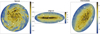 |
Fig. 1 HPN reference images of the Au-16 galaxy at λ = 7.88 µm, viewed at face-on (right), edge-on (middle), and intermediate (right) angles. Colour indicates flux density in MJy sr−1, given in logarithmic scale. Numbers on spatial maps indicate positions of pixels whose SEDs are shown in Sect. 3.2.1. |
2.3.2 NMF
NMF is another unsupervised dimensionality reduction method widely used in various fields (e.g. Lee & Seung 1999; Tandon & Sra 2010). Similar to PCA, NMF decomposes the feature space of the training dataset into the product of two matrices with smaller ranks. One matrix represents the NMF features that are linear combinations of the original dataset features, while the second Non-negative matrix factorisation matrix contains coefficients or weights associated with NMF features. NMF is initiated by attributing guess values to the elements of the reduced rank matrices, which are then iteratively updated until both NMF matrices are stable and their product approaches the original training dataset. Although very similar to PCA, NMF has an additional requirement that both original and decomposed matrices have no negative elements. This property might be beneficial when treating data with only non-negative values, such as astronomical fluxes (Ren et al. 2018; Boulais et al. 2021). Here, we employed an nmf7 R function.
2.4 Implementation
We applied our method to the Au-16 galaxy, which represents a typical MW-type galaxy with well-resolved spiral structure. Figure 1 shows Au-16 galaxy viewed from different angles face-on, edge-on, and intermediate, at wavelength λ = 7.88 µm. These high-resolution synthetic images are the result of a SKIRT simulation performed with 3 × 10¹⁰ photon packages, which are hereafter referred to as the high photon number (HPN) reference images. The optimal number of photon packages used for HPN reference images has been previously tested by Kapoor et al. (2021), based on pixel-to-pixel relative error calculation. The authors have shown that simulations performed with 3 × 10¹⁰ photon packages provide sufficiently high signal-to-noise ratio for most of the bands, with the exception of certain low-flux regions in UV and sub-millimetre ranges. Those images are available as part of the SKIRT Auriga project8 , and we use them to evaluate the performance of our method. In addition, we ran SKIRT simulations of the same galaxy, but with a lower number of photon packages, 3 × 10⁸ and 3 × 10⁹, and used them as low photon number (LPN) input images. LPN input images require only ~2% and ~ll% of the HPN reference simulation execution time for 3 × 10⁸ and 3 × 10⁹ photon packages, respectively. This time scaling justifies the implementation of the methodology proposed here, capable of reproducing high-resolution synthetic observations using time-effective LPN images as an input.
Even though INLA provides a promising path to overcome the computational limits of SKIRT simulations, INLA reconstructions alone can also be time costly, especially for large data cubes such as in this particular case. The SKIRT simulation output of our dataset is a cube of 3072×3072 pixels at 50 wavelength bins, from 0.15 µm to 1.24mm. Initial conditions for SKIRT Auriga simulations are taken from the Auriga simulation snapshots, using a cubical aperture to extract the data. The aperture is centred at the galaxy centre, with a side length adjusted in a manner that it includes most of the bound galaxy particles, but at the same time avoids secondary structures, such as satellite galaxies. Kapoor et al. (2021) used the side length twice the radius at which the face-on stellar surface density within 10 kpc of the mid plane falls below the threshold value 2 × 10⁵ M⊙ kpc−2. Since the same cubic aperture is used for all three inclinations, edge-on images will have extended regions with essentially no information. In post-processing, we decided to exclude those outermost pixels, resulting with different cube dimensions: 2150×2150×50 for the face-on cube; 2400×900×50 for the edge-on cube, and 1800×2200×50 for the intermediate cube.
Full data cube reconstruction requires 50 individual spatial reconstructions, one for each of the wavelength bins. Such reconstructions are labelled ‘pure INLA’ in the following text. We employed PCA and NMF techniques to reduce the number of dimensions, that is the number of individual spatial maps to be reconstructed with INLA. Both methods transform the original dataset in the spectral dimension, such that these spectra are described with a new orthogonal basis (in order of decreasing variability) instead of the 50 wavelengths. In this transformed space, the first components will carry most of the information, while the rest are responsible for less prominent features and noise, and can be discarded in order to trade some of the precision for efficiency. After performing PCA or NMF transformation on the initial variables (wavelength bins), these are replaced by a reduced number of principal components, whose maps are used as input to INLA. INLA then reconstructs the spatial maps of the coefficients attached to our selected set of principal components, instead of flux densities from the original data cube. Reconstructed spatial maps are then multiplied by the transpose of the principal components, resulting in the reconstructed data cube with the original dimensions, labelled ‘PCA or NMF with INLA’ reconstructions. In Appendix A, we show spatial maps of PCA and NMF components before and after INLA reconstructions. In Appendix B, we compare PCA and NMF reconstructions before and after applying INLA. Pure PCA or NMF reconstructions show higher residuals compared to PCA or NMF with INLA reconstructions.
Additionally, the INLA spatial reconstruction time can be reduced by sampling the input map data, instead of using complete spatial information. INLA shows optimal performance when applied to sparse data, the execution time is notably reduced, while the quality of reconstructions is influenced only to a lesser degree (González-Gaitán et al. 2019). This is further studied in Sect. 3.1, where we perform INLA reconstructions using different sampling percentages. We also test a different number of PCA or NMF components in order to find an optimal compromise between the quality of reconstructed maps and the required running times.
3 Results and discussion
3.1 Field cuts optimisation
We tested the optimal pixel sampling percentage using the 600 × 600 × 50 cut of the face-on cube. The quality of INLA reconstructions, compared to HPN reference images, is quantified by the normalised residuals, calculated as

where X′ and X refer to INLA reconstruction and HPN reference images, respectively.
Figure 2 presents the median of normalised residuals of pure INLA reconstructions as a function of the sampling percentage used (5%, 10%, 25%, 50%, and 100%) for the 600 × 600 × 50 cut. The total running times for INLA reconstructions are represented with different colours. Horizontal lines refer to the median residuals of the LPN inputs in relation to the HPN reference image without applying INLA, for 3 × 10⁸ (circles) and 3 × 10⁹ (triangles) photon number simulations.
Increasing the sample size improves the quality of reconstructions at the cost of a higher computational time. In terms of balance between residuals and the running times, INLA shows the optimal performances when applied to sparse data. Figure 2 shows that using more than 25% of the spatial data as INLA input significantly increases the running times with only a lesser (1–2%) improvement in the quality of reconstructions. In the following sections, we present reconstructions using 10% and 25% of the spatial information.
Next, we explore the optimal number of PCA or NMF components. PCA and NMF analyses were performed using 100% of data within the 600 × 600 × 50 cut, followed by sampling a percentage (10% or 25%) of spatial maps of PCA or NMF coefficients as an input to INLA. Figure 3 represents the median of normalised residuals as a function of the number of PCA or NMF components used for the reconstruction. The figure shows a clear improvement in reconstructions when more than two components are used, followed by a more gradual change. This behaviour suggests that the first components describe the overall structure and major features, while others represent for instance diffuse emission and low flux regions. In the case of PCA, a small decrease in residuals is noticed up to the tenth component, while using more than ten PCA or NMF components does not improve the results. However, NMF does not show such a clear trend, and using between 4 and 12 components only results in an ~0.5% change in median residuals.
Application of our methodology to this field cut shows that using dimensionality reduction techniques prior to INLA drastically reduces the total computation time of the proposed post-processing technique without loss of precision. Additionally, even the quality of reconstructions is improved compared to pure INLA (horizontal lines in Fig. 3) if more than two components are used.
Next, we move to the full field processing. Reconstructions of full cube images shown in the following section were performed using 10 PCA or NMF components, with data sampling of 10% and 25%.
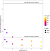 |
Fig. 2 Median of normalised residuals of pure INLA reconstruction as a function of sampling percentage for the 600 × 600 × 50 cut of a face-on cube. Circles and triangles refer to 3 × 10⁸ and 3 × 10⁹ photon number realisations, respectively. Horizontal lines refer to LPN input without spatial inference to HPN reference residuals. The total running times are represented in different colours. |
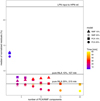 |
Fig. 3 Median of normalised residuals of PCA or NMF with INLA reconstruction as a function of a number of PCA or NMF components used for the reconstruction, resulting from sampling 10% and 25% from 3 × 10⁸ photon number realisation. |
3.2 Full field processing
In this section, we present the results for full field reconstructions using pure INLA and PCA or NMF with INLA techniques. We teste our method using LPN SKIRT simulations (3 × 10⁸ and 3 × 10⁹ photon packages) with different inclination angles: face-on, edge-on, and intermediate. INLA reconstructions are performed using 10% or 25% of the available spatial information. All figures shown in this section refer to reconstructions using 25% of the LPN (3 × 10⁸) input data, while the complete statistics of full field processing are summarised in Tables 1 and 2.
3.2.1 Spectral reconstructions
In this section, we explore how the reconstructed images follow the expected SED of the HPN reference. First, we compare the spatially integrated SEDs, obtained from integrating all flux at each wavelength bin. Figure 4 shows integrated SEDs for HPN reference (o), pure INLA (+), PCA with INLA (×), and NMF with INLA (◊), (upper panels) with the associated residuals (lower panels), for face-on (left), edge-on (middle), and intermediate (right) cubes. For each of the employed techniques, integrated SEDs provide a good match to the HPN reference, throughout the whole wavelength range. PCA with INLA reconstructions display the highest deviations from the expected SEDs at wavelengths around 100 µm, up to ~1.5 % for face-on and edge-on cubes, and ~3% for the intermediate cube.
Table 1 summarises the statistics for all of the employed realisations: face-on, edge-on, and intermediate cubes, simulated using 3 × 10⁸ and 3 × 10⁹ photon packages. Medians of the normalised residual percentages are shown for pure INLA and PCA or NMF with INLA integrated SEDs, compared to the HPN reference. Predicted integrated SEDs are in excellent agreement with the expectations, with the median of the normalised residuals being ≲0.1% for pure INLA and NMF with INLA reconstructions and ≲0.3% for PCA with INLA.
Next, we explore how the quality of our predictions changes at various regions throughout the galaxy plane. We inspected SEDs for individual spaxels9 whose spatial positions are marked in Fig. 1. The chosen spaxels occupy different regions of galaxy morphology, such as central parts, strong spiral arms, low flux density regions between spiral arms and galaxy outskirts. Figures 5, 6, and 7 show single-spaxel SEDs for face-on, edge-on, and intermediate cubes, respectively, sampling 25% of 3 × 10⁸ photon number realisation.
Both pure INLA (green) and PCA or NMF with INLA (blue and cyan lines) reconstructions are generally in good agreement with HPN reference SEDs (black lines) for most pixel positions. The quality of reconstructions is correlated with the spaxel position and the flux density. At high flux density regions, such as central parts and prominent spiral arms, LPN input SEDs (red lines) closely follow the HPN reference, and each of the employed techniques provides accurate predictions (spaxels at positions 1 and 2). At lower flux densities along spiral arms (spaxels 3 and 4), LPN input becomes noisy; however, the quality of our reconstructions is not affected. Yet, the reconstruction of the faint, outermost parts of the galaxy (spaxels 5 and 6) becomes challenging given the LPN input SEDs with both noisy and missing data. In these regions, pure INLA and NMF with INLA are, overall, able to recover the full SED of the HPN reference cube, while PCA with INLA occasionally fails in the reconstruction, resulting in non-physical negative flux densities. Such an example is shown in Fig. 6, where the LPN input spaxel is not complete, meaning it has zero values at some wavelengths. PCA with INLA reconstruction fails for spaxel 6, positioned at the galaxy outskirt. The NMF with INLA SED is complete; however, the reconstructions overestimate the HPN reference SED, while pure INLA provides the best match. In Table 2, we provide summary of the median of the normalised residuals and the computation time of each methodology.
Median of the normalised residuals for integrated SEDs from pure INLA and PCA or NMF with INLA reconstructions using different sampling percentages (10% and 25%) of 3 × 10⁸ and 3 × 10⁹ photon number cubes.
Median of the normalised residuals and the running times for each realisation, compared to HPN reference.
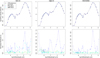 |
Fig. 4 Integrated SEDs for HPN reference, pure INLA, and PCA or NMF with INLA reconstructions (upper panels) with the associated residuals (lowerpanels), for face-on (left), edge-on (middle), and intermediate (right) cubes. |
3.2.2 Spatial reconstructions
Figures in this section show spatial distribution of randomly sampling 25% of the LPN input cube spaxels, together with pure INLA and PCA or NMF with INLA reconstructions (upper panels). Each of these cubes is compared to the HPN reference and normalised residuals are shown in the lower panels. Figures 8–11 show spatial reconstructions of the face-on cube at four wavelength bins: 0.23 µm, 7.88 µm, 100.08 µm, and 515.36 µm. Figures 12 and 13 show edge-on and ‘intermediate cubes’ at the wavelength bin 7.88 µm.
By using a sample of LPN input cube our methods are able to recover underlying spatial information and reveal structures seen on HPN reference images (Fig. 1). The quality of reconstructions is quantified by the median of normalised residuals (%), calculated for each pixel at the given wavelength bin, and shown above each residual reconstruction image. The pure INLA results generally display the lowest residuals; however, this technique’s extensive running time disqualifies it as a viable route to emulate MCRT codes. The PCA or NMF with INLA reconstructions have similar residuals, with ≲25% of the running time required for HPN reference (Table 2). However, at certain wavelength bins, the PCA with INLA technique fails in the reconstruction of ~ 10% of spatial information, positioned at regions with the lowest flux density. Those regions with non-physical negative flux densities can be seen in Figs. 10, 12, and 13 as white pixels. The problem with non-physical reconstructions induced by PCA analysis can be avoided using NMF instead, since NMF enforces only positive elements in both original and decomposed matrices. Using the NMF with INLA method, the problematic regions are reconstructed, but with typically higher residuals compared to pure INLA.
Figure 14 shows the median of normalised residuals as a function of wavelength for face-on (left), edge-on (middle), and intermediate (right) cubes. Although similar to Fig. 4, which shows normalised residuals for integrated SEDs, here we calculate residuals for each pixel at a given wavelength bin separately and then calculate their median value. Pixels with negative values are converted to zero, resulting in normalised residuals of 100% (Eq. (13)). Overall, all of the employed methods (pure INLA and PCA or NMF with INLA) result in significantly lower residuals compared to LPN input. Pure INLA (green) is able to recover spatial information over the whole range of wavelength bins, with the median of normalised residuals being ≲20 % for a face-on cube and ≲30% for edge-on and intermediate cubes. On the other side, both PCA or NMF with INLA reconstructions have higher residuals at wavelengths of ~20–150 µm. At these wavelengths, both LPN input and HPN reference images lose diffuse emission of low intensity that fills regions between the spiral structure, otherwise present at other wavelength bins. PCA and NMF components carry information about this diffuse emission and will always try to reconstruct it, resulting in higher residuals at wavelengths where the emission is attenuated in the original images. However, statistics for these wavelength bins is governed by outskirt regions of the galaxy where PCA with INLA reconstructions fail, while NMF with INLA overestimates the flux density. When applied to a field cut that includes the galaxy central region, both the PCA or NMF with INLA methods result in lower residuals compared to the pure INLA technique (Fig. 3). Thus, masking out the outskirt regions prior to INLA would improve the reconstructions.
 |
Fig. 5 Single-spaxel SEDs for HPN reference (black) and LPN input (red) face-on cubes, together with pure INLA (green) and PCA or NMF with INLA (blue and cyan) reconstructions. Spatial positions of the spaxels represented here are shown in Fig. 1. |
3.3 Summary and discussion
Table 2 summarises statistics for the spatial reconstructions of face-on, edge-on, and intermediate cubes, using pure INLA and PCA or NMF with INLA implementations. We present results for two different LPN input images (3 × 10⁸ and 3 × 10⁹ photon number), using a randomly sampled 10% or 25% of the available spatial information. Both LPN input images and the reconstructions are compared to the HPN reference. The median of the normalised residuals are shown for each cube, together with the total running time required for LPN SKIRT simulations and INLA reconstructions. Running times presented in Table 2 are as follows:

where tINLA refers either to pure INLA reconstructions (50 images at 50 wavelength bins) or to the total time for PCA or NMF analysis with INLA reconstructions.
For each realisation, residuals for our reconstructions are significantly lower compared to LPN input residuals, proving that each of the employed methods is able to recover spatial structure using only 10% or 25% of the LPN input. Although pure INLA reconstructions result in the lowest residuals, this methodology does not provide a significant acceleration. Using a sample size of 10% requires ≳70% of the HPN reference SKIRT running time, while using 25% of the face-on cube exceeds it. However, employing dimensionality reduction techniques successfully reduces the running times for up to ~10% of HPN reference’s with similar residuals.
Additionally, the quality of our reconstructions scales with LPN input residuals; thus, the face-on cube has overall lower residuals compared to other tilt angles. Depending on the LPN input (3 × 10⁸ or 3 × 10⁹ photon number) and the sample size (10% or 25%), residuals of PCA or NMF with INLA reconstructions are in the range of ~10–20% for the face-on cube and ~15–30% for the edge-on and intermediate cubes. Naturally, the lowest residuals are achieved when using 25% of the 3 × 10⁹ photon number LPN input cube, which requires ~25–40% of the HPN reference running time. At the other end, by sampling 10% of the 3 × 10⁸ photon number LPN input cube, the running times are reduced to ~7–20% of the HPN reference. The edge-on cube typically has shorter running times due to a smaller size field (2401 × 901 × 50), compared to the face-on cube (2151 × 2151 × 50).
When applied to a field cut, the PCA with INLA method outperforms pure INLA, both by lower residuals and significantly shorter running times (Fig. 3), since this cut does not include galaxy outskirts. This proves that performing a careful prior segmentation of the galaxy or astrophysical source will aid best in our post-processing technique. Furthermore, PCA analysis has advantages over NMF: PCA analysis is faster, and the number of PCA components does not need to be decided in advance. On the other hand, NMF always provides physically positive reconstructions, which are particularly useful at low flux regions like the outskirts of the image.
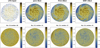 |
Fig. 8 Spatial distribution of LPN input cube and pure INLA, PCA or NMF with INLA reconstructions (upperpanels) with the associated residuals (bottompanels) at wavelength bin 0.23 µm. Sample size: 25%, face-on cube. Colour legends are given in logarithmic scale. |
4 Conclusions
In this work, we used PCA and NMF dimensionality reduction techniques together with approximate Bayesian inference of continuous Gaussian random fields with INLA for SKIRT simulation post-processing. We tested our methodology using three images of the Au-16 SKIRT Auriga galaxy, simulated with different tilt angles: face-on, edge-on, and intermediate. These HPN reference images (3 × 10¹⁰ photon packages) served as the ‘ground truth’ to which we compared the performance of our method applied to LPN input images ( 3 × 10⁸ or 3 × 10⁹ photon packages).
Our results showed that spatially integrated SEDs closely follow the reference SED for each of the employed methods, with the median of the normalised residuals typically being ≲0.3%. Spatial modelling suggests that the quality of our reconstructions changes with the position along the galaxy plane, with faint galaxy outskirts having the highest residuals.
Depending on the number of photon packages, the sample size, and the desired quality of reconstruction, our method offers time-efficient reconstructions with spatial residuals of ~20–30%, requiring ~7–20% of the HPN reference running time. Higher quality reconstructions can be achieved by sampling 25% of the 3 × 10⁹ LPN input image, resulting in residuals of ~ 10–20% within ~20–40% of the HPN reference running time.
In order to improve the quality of reconstructions, different sampling methods based on information on the spatial densities and different pre-INLA data pre-processing might be worth exploring. Even though our results are not sensitive to the choice of sampling method (random or uniform), more complex and less homogeneous spatial maps might require non-uniform sampling.
Being able to efficiently perform large amounts of numerical simulations with varying physical characteristics is essential to compare to real observations in a quantitative way. Even if the accuracy is not immediately as good as that of an HPN simulation, such explorations with optimised LPN simulations can help narrow down the parameters to then run a full HPN simulation. This work represents a crucial step in this direction.
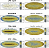 |
Fig. 12 Edge-on cube at wavelength bin 7.88 µm. |
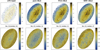 |
Fig. 13 ‘Intermediate’ cube at wavelength bin 7.88 µm. |
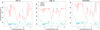 |
Fig. 14 Median of normalised residuals as a function of wavelength for face-on (left), edge-on (middle), and intermediate (right) cubes. |
Acknowledgements
We acknowledge the support by the programme of scientific and technological cooperation between the government of the Republic of Serbia and the government of the Republic of Portugal, (grant no. 337-00-00227/201909/53 and FCT 5581 DRI, Sérvia 2020/21). M.S. and M.S. acknowledge support by the Science Fund of the Republic of Serbia, PROMIS 6060916, BOWIE and by the Ministry of Education, Science and Technological Development of the Republic of Serbia through the contract no. 451-03-9/2022-14/200002. J.R.-S. is funded by Fundação para a Ciência e a Tecnologia (PD/BD/150487/2019), via the International Doctorate Network in Particle Physics, Astrophysics and Cosmology. S.G.G and J.R.-S. acknowledge the support of FCT under Project CRISP PTDC/FIS-AST-31546/2017.
Appendix A Spatial reconstructions of PCA and NMF components
Here, we further explore the reconstructions obtained using PCA and NMF methods. Figures A.1 and A.2 show examples of spatial maps of PCA and NMF coefficients attached to principal components before INLA (left panels) and after INLA (right panels). PCA sorts principal components by the amount of information they carry, which can be seen in Figure A.1. The first component reconstructs the highest flux density regions: galaxy centre and strong spiral structure. The second principal component reconstructs outer parts of the spiral arms and the galaxy outskirts. The remaining principal components reconstruct background emission and less prominent features in the spiral structure. Up to the sixth principal component, INLA reconstructions do not significantly differ from the input. However, for the remaining principal components INLA reconstructions predict less variability, which is especially evident for the sixth component.
On the other hand, NMF components are not sorted by the amount of variability. Figure A.2 shows that NMF components can be distinguished between those that reconstruct central parts, a spiral structure, and a mixture of different features. Overall, the structure seen in all NMF components is preserved and slightly highlighted after INLA reconstructions.
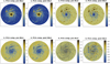 |
Fig. A.1 Spatial maps of PCA coefficients attached to principal components before INLA (left panels) and after INLA (right anels). Sample size: 25%, face-on cube. |
Appendix B Pure PCA and NMF reconstructions
In this section, we compare PCA (Figure B.1) and NMF (Figure B.2) reconstructions before and after INLA. Figures B.1 and B.2 show pure PCA or NMF and PCA or NMF with INLA reconstructions (upper panels) and the associated residuals (lower panels) at different wavelength bins: 0.23 µm, 7.88 µm, 100.08 µm, and 515.36 µm. Pure PCA or NMF reconstructions refer to results of PCA or NMF analyses performed using 100% of full LPN input cube and ten PCA or NMF components. The quality of these reconstructions is further enhanced with INLA using a randomly sampled 25% of the PCA or NMF coefficients. Results of both pure PCA or NMF and PCA or NMF with INLA reconstructions are compared to HPN reference images.
Figure B.1 shows that a pure PCA method produces pixels with negative values. PCA or NMF with INLA reconstructions result in lower residuals compared to the pure PCA or NMF technique. Employing INLA reduces the amount of negative reconstructions leading to lower residuals and thus better quality reconstructions. However, at wavelengths of ~100 µm, the amount of negative values is still high after INLA, leading to higher residuals at the galaxy outskirts. On the other hand, NMF reconstructions (Figure B.2) do not suffer from non-physically negative reconstructions; yet, at the same wavelength bins (~100 µm ) NMF with INLA overestimate flux densities at the galaxy outskirts, leading to higher residuals compared to pure NMF reconstructions.
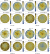 |
Fig. B.1 Pure PCA and PCA with INLA spatial reconstructions (upper panels) and the associated residuals (lower panels) at the following wavelength bins: 0.23µm, 7.88 µm, 100.08 µm, and 515.36µm. Sample size: 25%, face-on cube. |
References
- Baes, M., & Camps, P. 2015, Astron. Comput., 12, 33 [NASA ADS] [CrossRef] [Google Scholar]
- Baes, M., Fritz, J., Gadotti, D. A., et al. 2010, A&A, 518, A39 [Google Scholar]
- Behrens, C., Pallottini, A., Ferrara, A., Gallerani, S., & Vallini, L. 2018, MNRAS, 477, 552 [NASA ADS] [CrossRef] [Google Scholar]
- Boulais, A., et al. 2021, A&A, 647, A105 [NASA ADS] [CrossRef] [EDP Sciences] [Google Scholar]
- Bruzual, G., & Charlot, S. 2003, MNRAS, 344, 1000 [NASA ADS] [CrossRef] [Google Scholar]
- Camps, P., & Baes, M. 2015, Astron. Comput., 9, 20 [Google Scholar]
- Camps, P., Kapoor, A. U., Trcka, A., et al. 2022, MNRAS, 512, 2728 [NASA ADS] [CrossRef] [Google Scholar]
- Collins, J. D., Hart, G. C., Haselman, T. K., & Kennedy, B. 1974, AIAA J., 12, 185 [NASA ADS] [CrossRef] [Google Scholar]
- Crain, R. A., Schaye, J., Bower, R. G., et al. 2015, MNRAS, 450, 1937 [NASA ADS] [CrossRef] [Google Scholar]
- De Geyter, G., Baes, M., De Looze, I., et al. 2015, MNRAS, 451, 1728 [NASA ADS] [CrossRef] [Google Scholar]
- De Looze, I., Baes, M., Bendo, G. J., et al. 2012a, MNRAS, 427, 2797 [NASA ADS] [CrossRef] [Google Scholar]
- De Looze, I., Baes, M., Fritz, J., & Verstappen, J. 2012b, MNRAS, 419, 895 [NASA ADS] [CrossRef] [Google Scholar]
- Deeley, S., Drinkwater, M. J., Sweet, S. M., et al. 2021, MNRAS, 508, 895 [NASA ADS] [CrossRef] [Google Scholar]
- Di Mascia, F., Gallerani, S., Ferrara, A., et al. 2021, MNRAS, 506, 3946 [NASA ADS] [CrossRef] [Google Scholar]
- Dudzeviciute, U., Smail, I., Swinbank, A. M., et al. 2020, MNRAS, 494, 3828 [NASA ADS] [CrossRef] [Google Scholar]
- Font, A. S., McCarthy, I. G., Poole-Mckenzie, R., et al. 2020, MNRAS, 498, 1765 [NASA ADS] [CrossRef] [Google Scholar]
- Genel, S., Vogelsberger, M., Springel, V., et al. 2014, MNRAS, 445, 175 [Google Scholar]
- Gómez-Rubio, V. 2021, Bayesian Inference with INLA (Boca Raton, FL: Chapman & Hall/CRC Press) [Google Scholar]
- Gong, W., Reich, B. J., & Chang, H. H. 2021, Environ. Res. Commun., 3, 101002 [NASA ADS] [CrossRef] [Google Scholar]
- González-Gaitán, S., de Souza, R. S., Krone-Martins, A., et al. 2019, MNRAS, 482, 3880 [CrossRef] [Google Scholar]
- Grand, R. J. J., Gómez, F. A., Marinacci, F., et al. 2017, MNRAS, 467, 179 [NASA ADS] [Google Scholar]
- Groves, B., Dopita, M. A., Sutherland, R. S., et al. 2008, ApJS, 176, 438 [NASA ADS] [CrossRef] [Google Scholar]
- Hotelling, H. 1933, J. Educ. Psychol., 24, 417 [CrossRef] [Google Scholar]
- Jaffé, R., Nunes, S., Filipe Dos Santos, J., et al. 2021, Environ. Res. Lett., 16, 084034 [CrossRef] [Google Scholar]
- Jolliffe, I. T., & Cadima, J. 2016, Philos. Trans. Roy. Soc. London A, 374, 20150202 [NASA ADS] [Google Scholar]
- Jones, A. P., Köhler, M., Ysard, N., Bocchio, M., & Verstraete, L. 2017, A&A, 602, A46 [NASA ADS] [CrossRef] [EDP Sciences] [Google Scholar]
- Kapoor, A. U., Camps, R., Baes, M., et al. 2021, MNRAS, 506, 5703 [NASA ADS] [CrossRef] [Google Scholar]
- Krone-Martins, A., & Moitinho, A. 2014, A&A, 561, A57 [NASA ADS] [CrossRef] [EDP Sciences] [Google Scholar]
- Lee, D., & Seung, H. 1999, Nature, 401, 788 [NASA ADS] [CrossRef] [Google Scholar]
- Logan, C. H. A., & Fotopoulou, S. 2020, A&A, 633, A154 [NASA ADS] [CrossRef] [EDP Sciences] [Google Scholar]
- Noebauer, U. M., & Sim, S. A. 2019, Living Rev. Comput. Astrophys., 5, 1 [CrossRef] [Google Scholar]
- Pearson, K. 1901, London Edinburgh Dublin Philos. Mag. J. Sci., 2, 559 [CrossRef] [Google Scholar]
- Pillepich, A., Springel, V., Nelson, D., et al. 2018, MNRAS, 473, 4077 [Google Scholar]
- Ren, B., et al. 2018, ApJ, 852, 104 [NASA ADS] [CrossRef] [Google Scholar]
- Rino-Silvestre, J., González-Gaitán, S., Stalevski, M., et al. 2022, Neural Comput & Applic (2022), https://doi.org/1S.1S07/sSS521-S22-S8S71-x [Google Scholar]
- Rowland, B. W., Rushton, S. P., Shirley, M. D. F., Brown, M. A., & Budge, G. E. 2021, Sci. Rep., 11, 21953 [NASA ADS] [CrossRef] [Google Scholar]
- Rue, H., Martino, S., & Chopin, N. 2009, J. Roy. Stat. Soci. B (Stat. Methodol.), 71, 319 [CrossRef] [Google Scholar]
- Rue, H., Riebler, A., Sørbye, S. H., et al. 2017, Annu. Rev. Stat. Applic., 4, 395 [NASA ADS] [CrossRef] [Google Scholar]
- Schaye, J., Crain, R. A., Bower, R. G., et al. 2015, MNRAS, 446, 521 [Google Scholar]
- Springel, V. 2010, MNRAS, 401, 791 [Google Scholar]
- Stalevski, M., Ricci, C., Ueda, Y., et al. 2016, MNRAS, 458, 2288 [Google Scholar]
- Stalevski, M., Asmus, D., & Tristram, K. R. W. 2017, MNRAS, 472, 3854 [NASA ADS] [CrossRef] [Google Scholar]
- Stalevski, M., Tristram, K. R. W., & Asmus, D. 2019, MNRAS, 484, 3334 [NASA ADS] [CrossRef] [Google Scholar]
- Steinacker, J., Baes, M., & Gordon, K. D. 2013, ARA&A, 51, 63 [CrossRef] [Google Scholar]
- Tandon, R., & Sra, S. 2010, Sparse nonnegative matrix approximation: new formulations and algorithms, Tech. Rep. 193, Max Planck Institute for Biological Cybernetics, Tübingen, Germany [Google Scholar]
- Van Niekerk, J., Bakka, H., Rue, H., & Schenk, O. 2021, J. Stat. Softw., 100, 1 [CrossRef] [Google Scholar]
- Vijayan, A. P., Wilkins, S. M., Lovell, C. C., et al. 2022, MNRAS, 511, 4999 [NASA ADS] [CrossRef] [Google Scholar]
- Vogelsberger, M., Genel, S., Sijacki, D., et al. 2013, MNRAS, 436, 3031 [Google Scholar]
- Vogelsberger, M., Genel, S., Springel, V., et al. 2014a, Nature, 509, 177 [Google Scholar]
- Vogelsberger, M., Genel, S., Springel, V., et al. 2014b, MNRAS, 444, 1518 [Google Scholar]
- Weinberger, R., Springel, V., Hernquist, L., et al. 2017, MNRAS, 465, 3291 [Google Scholar]
- Whitney, A., Ferreira, L., Conselice, C. J., & Duncan, K. 2021, ApJ, 919, 139 [NASA ADS] [CrossRef] [Google Scholar]
- Zanella, A., Pallottini, A., Ferrara, A., et al. 2021, MNRAS, 500, 118 [Google Scholar]
For a full list, see https://skirt.ugent.be/root/_publications_all_date.html
All Tables
Median of the normalised residuals for integrated SEDs from pure INLA and PCA or NMF with INLA reconstructions using different sampling percentages (10% and 25%) of 3 × 10⁸ and 3 × 10⁹ photon number cubes.
Median of the normalised residuals and the running times for each realisation, compared to HPN reference.
All Figures
|
Fig. 1 HPN reference images of the Au-16 galaxy at λ = 7.88 µm, viewed at face-on (right), edge-on (middle), and intermediate (right) angles. Colour indicates flux density in MJy sr−1, given in logarithmic scale. Numbers on spatial maps indicate positions of pixels whose SEDs are shown in Sect. 3.2.1. |
| In the text | |
|
Fig. 2 Median of normalised residuals of pure INLA reconstruction as a function of sampling percentage for the 600 × 600 × 50 cut of a face-on cube. Circles and triangles refer to 3 × 10⁸ and 3 × 10⁹ photon number realisations, respectively. Horizontal lines refer to LPN input without spatial inference to HPN reference residuals. The total running times are represented in different colours. |
| In the text | |
|
Fig. 3 Median of normalised residuals of PCA or NMF with INLA reconstruction as a function of a number of PCA or NMF components used for the reconstruction, resulting from sampling 10% and 25% from 3 × 10⁸ photon number realisation. |
| In the text | |
|
Fig. 4 Integrated SEDs for HPN reference, pure INLA, and PCA or NMF with INLA reconstructions (upper panels) with the associated residuals (lowerpanels), for face-on (left), edge-on (middle), and intermediate (right) cubes. |
| In the text | |
|
Fig. 5 Single-spaxel SEDs for HPN reference (black) and LPN input (red) face-on cubes, together with pure INLA (green) and PCA or NMF with INLA (blue and cyan) reconstructions. Spatial positions of the spaxels represented here are shown in Fig. 1. |
| In the text | |
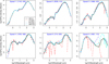 |
Fig. 6 Same as Fig. 5, but for edge-on cube. |
| In the text | |
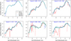 |
Fig. 7 Same as Fig. 5, but for intermediate cube. |
| In the text | |
|
Fig. 8 Spatial distribution of LPN input cube and pure INLA, PCA or NMF with INLA reconstructions (upperpanels) with the associated residuals (bottompanels) at wavelength bin 0.23 µm. Sample size: 25%, face-on cube. Colour legends are given in logarithmic scale. |
| In the text | |
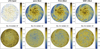 |
Fig. 9 Same as Fig. 8, but at wavelength bin 7.88 µm. |
| In the text | |
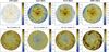 |
Fig. 10 Same as Fig. 8, but at wavelength bin 100.80 µm. |
| In the text | |
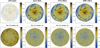 |
Fig. 11 Same as Fig. 8, but at wavelength bin 515.36 µm. |
| In the text | |
|
Fig. 12 Edge-on cube at wavelength bin 7.88 µm. |
| In the text | |
|
Fig. 13 ‘Intermediate’ cube at wavelength bin 7.88 µm. |
| In the text | |
|
Fig. 14 Median of normalised residuals as a function of wavelength for face-on (left), edge-on (middle), and intermediate (right) cubes. |
| In the text | |
|
Fig. A.1 Spatial maps of PCA coefficients attached to principal components before INLA (left panels) and after INLA (right anels). Sample size: 25%, face-on cube. |
| In the text | |
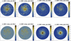 |
Fig. A.2 Same as Fig. A.1, for NMF method. |
| In the text | |
|
Fig. B.1 Pure PCA and PCA with INLA spatial reconstructions (upper panels) and the associated residuals (lower panels) at the following wavelength bins: 0.23µm, 7.88 µm, 100.08 µm, and 515.36µm. Sample size: 25%, face-on cube. |
| In the text | |
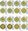 |
Fig. B.2 Same as Fig. B.1, but for pure NMF and NMF with INLA reconstructions. |
| In the text | |
Current usage metrics show cumulative count of Article Views (full-text article views including HTML views, PDF and ePub downloads, according to the available data) and Abstracts Views on Vision4Press platform.
Data correspond to usage on the plateform after 2015. The current usage metrics is available 48-96 hours after online publication and is updated daily on week days.
Initial download of the metrics may take a while.