| Issue |
A&A
Volume 691, November 2024
|
|
|---|---|---|
| Article Number | A356 | |
| Number of page(s) | 17 | |
| Section | Extragalactic astronomy | |
| DOI | https://doi.org/10.1051/0004-6361/202451200 | |
| Published online | 26 November 2024 | |
Transverse clues on the kiloparsec-scale structure of the circumgalactic medium as traced by C IV absorption
1
Departamento de Astronomía, Universidad de Chile, Casilla 36-D, Santiago, Chile
2
Kapteyn Astronomical Institute, University of Groningen, Landleven 12, 9747 AD Groningen, The Netherlands
3
Dipartimento di Fisica e Astronomia, Università di Firenze, Via G. Sansone 1, 50019 Sesto Fiorentino, Firenze, Italy
4
Instituto de Física, Pontificia Universidad Católica de Valparaíso, Casilla, 4059 Valparaíso, Chile
5
European Southern Observatory, Alonso de Córdova, 3107 Vitacura, Casilla, 19001 Santiago, Chile
6
Instituto de Astrofísica, Pontificia Universidad Católica de Chile, Av. Vicuña Mackenna 4860, 7820436 Macul, Santiago, Chile
7
NRC Herzberg Astronomy and Astrophysics Research Centre, 5071 West Saanich Road, Victoria, B.C. V9E 2E7, Canada
8
Instituto de Estudios Astrofísicos, Facultad de Ingeniería y Ciencias, Universidad Diego Portales, Av. Ejército Libertador 441, Santiago, Chile
9
Department of Physics, University of Cincinnati, Cincinnati, OH 45221, USA
10
French-Chilean Laboratory for Astronomy, IRL 3386, CNRS and U. de Chile, Casilla 36-D, Santiago, Chile
11
Centre de Recherche Astrophysique de Lyon, Université de Lyon 1, ENS-Lyon, UMR5574, 9 Av Charles André, 69230 Saint-Genis-Laval, France
12
Institut d’Astrophysique de Paris, CNRS-SU, UMR 7095, 98bis bd Arago, 75014 Paris, France
⋆ Corresponding author; This email address is being protected from spambots. You need JavaScript enabled to view it.
Received:
20
June
2024
Accepted:
3
October
2024
Abstract
The kiloparsec-scale kinematics and density structure of the circumgalactic medium (CGM) is still poorly constrained observationally, which poses a problem for understanding the role of the baryon cycle in galaxy evolution. Here we present VLT/MUSE integral-field spectroscopy (R ≈ 1800) of four giant gravitational arcs exhibiting W0 ≳ 0.2 Å C IV absorption at eight intervening redshifts, zabs ≈ 2.0–2.5. We detected C IV absorption in a total of 222 adjacent and seeing-uncorrelated sight lines whose spectra sample beams of (“de-lensed”) linear size ≈1 kpc. Our data show that (1) absorption velocities cluster at all probed transverse scales, Δr⊥ ≈ 0–15 kpc, depending on system; (2) the (transverse) velocity dispersion never exceeds the mean (line-of-sight) absorption spread; and (3) the (transverse) velocity autocorrelation function does not resolve kinematic patterns at the above spatial scales, but its velocity projection, ξarc(Δv), exhibits a similar shape to the known two-point correlation function toward quasars, ξQSO(Δv). An empirical kinematic model suggests that these results are a natural consequence of wide-beam observations of an unresolved clumpy medium. Our model recovers both the underlying velocity dispersion of the clumps (70–170 km s−1) and the mean number of clumps per unit area (2–13 kpc−2). The latter constrains the projected mean inter-clump distance to within ≈0.3–0.8 kpc, which we argue is a measure of clump size for a near-unity covering fraction. The model is also able to predict ξarc(Δv) from ξQSO(Δv), suggesting that the strong systems that shape ξarc(Δv) and the line-of-sight velocity components that define ξQSO(Δv) trace the same kinematic population. Consequently, the clumps must possess an internal density structure that generates both weak and strong components. We discuss how our interpretation is consistent with previous observations using background galaxies and multiple quasars as well as its implications for the connection between the small-scale kinematic structure of the CGM and galactic-scale accretion and feedback processes.
Key words: galaxies: evolution / galaxies: halos / galaxies: high-redshift / intergalactic medium / quasars: absorption lines
© The Authors 2024
 Open Access article, published by EDP Sciences, under the terms of the Creative Commons Attribution License (https://creativecommons.org/licenses/by/4.0), which permits unrestricted use, distribution, and reproduction in any medium, provided the original work is properly cited.
This article is published in open access under the Subscribe to Open model. This email address is being protected from spambots. You need JavaScript enabled to view it. to support open access publication.
1. Introduction
The widespread presence of metals in the diffuse intergalactic and circumgalactic media (IGM and CGM, respectively; e.g., Cowie et al. 1995; Ellison et al. 2000; Simcoe et al. 2004; Songaila 2005; Ryan-Weber et al. 2006; Becker et al. 2019; Cooper et al. 2019; D’Odorico et al. 2023; Bordoloi et al. 2024) suggests a continuous metal enrichment since z > 4 that remained constant until z = 2 (McQuinn 2016; D’Odorico et al. 2022; Galbiati et al. 2023). Produced in galaxies (e.g., Pettini et al. 2001; Adelberger et al. 2005; Lofthouse et al. 2023; Banerjee et al. 2023) and their environments (Shen et al. 2012), CGM metals enter a baryon cycle powered by galactic-scale feedback and re-accretion mechanisms that are believed to regulate star formation and ultimately galaxy evolution (e.g., Kereš et al. 2005; Oppenheimer & Davé 2008; Faucher-Giguère et al. 2011; Christensen et al. 2016). Both the outflowing (Rupke et al. 2005; Oppenheimer & Davé 2006) and inflowing (Nelson et al. 2015; Fielding et al. 2017; Faucher-Giguère & Oh 2023) gas may be clumpy, resulting in poor mixing of the metals on “small scales” (Schaye et al. 2007), defined here as ≲1 kpc. Thus, the CGM small-scale kinematics and spatial structure must be intimately connected to the baryon cycle of galaxies. Constraining the former observationally has become a cornerstone for understanding the latter and validating hydro simulations of increasingly higher resolution (e.g., Oppenheimer & Davé 2008; Wiersma et al. 2010; Cen & Chisari 2011; Rahmati et al. 2016; Bird et al. 2016; Finlator et al. 2020; Hummels et al. 2019; Peeples et al. 2019; Marra et al. 2024).
Measuring the clumpiness of the CGM is difficult because this medium is diffuse, and the rare bright background sources (e.g., quasars) required to detect it in absorption do not provide transverse sampling. The only option to directly probe the transverse dimension seems to rely on the even scarcer multiple background sources. In fact, resolved spectroscopy of lensed quasars and galaxies already have provided evidence that the T = 104 K enriched gas is clumpy on kiloparsec scales (Rauch et al. 1999, 2001a,b; Ellison et al. 2004; Lopez et al. 2005, 2007, 2018, 2020; Chen et al. 2014; Zahedy et al. 2016; Rubin et al. 2018a,b; Péroux et al. 2018; Krogager et al. 2018; Kulkarni et al. 2019; Zahedy et al. 2019; Mortensen et al. 2021; Bordoloi et al. 2022; Afruni et al. 2023).
An alternative way to probe the CGM structure on various scales is through measuring line-of-sight and transverse velocity clustering. This technique has been applied on different data sets, for instance, (i) the auto-correlation function of absorbers either along the line-of-sight at high spectral resolution (Steidel 1990; Pichon et al. 2003; Scannapieco et al. 2006; Boksenberg & Sargent 2015; Rauch et al. 1996; Fathivavsari et al. 2013) or transversely using lensed or multiple quasars in general (Rauch et al. 2001a; Coppolani et al. 2006; Tytler et al. 2009; Martin et al. 2010; Mintz et al. 2022; Maitra et al. 2019; Gontcho A Gontcho et al. 2018; Dutta et al. 2024; Hennawi et al. 2006); (ii) the absorber-galaxy cross-correlation either along the line-of-sight using background galaxies (Steidel et al. 2010; Turner et al. 2017) or transversely (Adelberger et al. 2005; Lofthouse et al. 2023; Banerjee et al. 2023; Galbiati et al. 2023); and (iii) other cross-correlations such as quasar-absorber (Hennawi & Prochaska 2007; Vikas et al. 2013) or outflow-absorber (Rauch et al. 2001b; Theuns et al. 2002). The broad picture that has emerged is that metals and galaxies trace the same overdensities. However, none of the observations can really disentangle the absorbing galaxy from the absorption system. Only a handful of them address the line-of-sight kinematics (e.g. Turner et al. 2017) and how this is supposed to be entangled with the spatial structure (Stern et al. 2016), and even fewer have really been able to measure the level of transverse structure (Rauch et al. 1999, 2001a,b).
In this article, we take advantage of multiplexed spectroscopy of giant gravitational arcs (hereafter “ARCTOMO1 data”) to measure the velocity clustering of intervening triply ionized carbon (C IV) across kiloparsec scales. The strong and easy-to-identify C IVλλ1548, 1550 doublet is arguably the most sensitive metal tracer of both the cool and warm CGM at high redshifts (Chen et al. 2001; Bordoloi et al. 2014; Rudie et al. 2019). On the other hand, ARCTOMO data have demonstrated the potential to add a wealth of unique and new spatial information on CGM scales (Lopez et al. 2018, 2020; Tejos et al. 2021; Fernandez-Figueroa et al. 2022; Afruni et al. 2023), hence the timely combination. We build on a blind survey of z ≈ 2 C IV in all available ARCTOMO fields (originally targeted for z ≈ 1 Mg II) that resulted in eight intervening C IV systems toward four arcs.
The paper is organized as follows. In Sect. 2, we describe the observations, the data reduction, and the spectrum extraction. Then in Sect. 3 we describe the automated C IV identification and line-profile fitting used, paying special attention to survey completeness, and in Sect. 4 we address the subtleties of dealing with lensed fields. We used these data for two kinds of analysis on C IV kinematics: First, in Sect. 5, we carry out a direct assessment of line-of-sight and transverse kinematic properties, and secondly, in Sect. 6, we measure transverse velocity clustering and compare it with quasar line-of-sight observations. Thereupon, in Sect. 7, we present a gas-kinematics model that explains the results, reproduces the arc signal out of the quasar kinematics, and predicts independent observations. Finally, in Sect. 8, we discuss the implications of our findings, concluding with a summary of the results in Sect. 9.
Throughout the paper we use a ΛCDM cosmology with the following cosmological parameters: H0 = 70 km s−1 Mpc−1, Ωm = 0.3, and ΩΛ = 0.7. We also use the standard notations  for a normal distribution with mean μ and variance σ2 and
 ![Mathematical equation: $ {\cal U}_{[a,b]} $](/articles/aa/full_html/2024/11/aa51200-24/aa51200-24-eq2.gif) for a continuous uniform distribution with support [a,b].
for a continuous uniform distribution with support [a,b].
2. ARCTOMO data
2.1. Observations
The four arcs were observed with the Multi Unit Spectroscopic Explorer (MUSE; Bacon et al. 2010) mounted on UT4 (Yepun) at the Very Large Telescope (VLT) in Paranal, Chile, as part of programs 297.A-5012 (PI Aghanim), 098.A-0459 (PI Lopez), and 0103.A-048 (PI Lopez). The observations were conducted in service mode with the MUSE wide field mode (WFM), which provides a field of view of 1′×1′ sampled at 0 2/spaxel. They used either non-adaptive optics and a nominal wavelength range (NOAO-N) or adaptive optics and an extended wavelength range (AO-E), depending on the program (Table 1). These setups provide spectral coverage of ≈4700–9300 Å and ≈4600–9300 Å respectively2, and a resolving power ranging from R ≃ 1770 at 4800 Å to R ≃ 3590 at 9300 Å. Exposure times varied between 0.8 and 4.2 hours. The requested image quality resulted in final point spread functions (PSFs) ranging from
  to
to  , depending on the targeted field.
Summary of targets and VLT/MUSE observations.
2.2. Data reduction
The data reduction was carried out using the ESO MUSE pipeline (v2.6, Weilbacher et al. 2020) in the ESO Recipe Execution Tool (EsoRex) environment (ESO CPL Development Team 2015). The master bias, flat field, and wavelength calibrations for each CCD were created from the associated raw calibrations, and they were applied to the raw science and standard-star observations as part of the pre-processing steps. Flux calibration was carried out using the standard star observations from the same nights as the science data, and the sky continuum was measured directly from the science exposures and subtracted off. The reduced data for each exposure were then stacked to produce the combined datacube, with a wavelength solution calibrated to vacuum. Any residual sky contamination was removed using the Zurich Atmosphere Purge code (ZAP, Soto et al. 2016). Finally, the datacubes were matched to the WCS of the corresponding HST data (references in Table 1). White-image stamps of the arcs are shown in the left-hand column of Fig. 1.
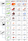 |
Fig. 1. MUSE arc images and C IV system maps. Columns from left to right: Column (1): White-image stamps of the gravitational arcs. Column (2): |

2.3. Binned spectra extraction
We extracted and combined the cube spectra optimally using 3 × 3 spaxel apertures (so binned spaxels are non-overlapping squares of 0 6 on a side), a size deemed sufficiently large to minimize cross-talk between adjacent spaxels due to seeing smearing, while maximizing spatial sampling (e.g., Lopez et al. 2018). We show in Appendix C that this choice does not bias our results. We considered an arc binned spectrum to sample an independent “arc sight line” or “arc beam.” By construction, these spectra have heterogeneous signal-to-noise ratios. Throughout the article, we apply appropriate completeness corrections to deal with each arc’s particular selection function.
3. Absorption line analysis and definitions
We defined a C IV “ARCTOMO system,” or simply a “C IV system,” as having significant C IV absorption detected in at least one arc sight line. We borrowed the concept of “system” from the quasar absorption lines technique despite the fact that here we deal with extended sources so that a system could be probed by several adjacent sight lines. In this article, we refer to intervening systems, c|zabs − zem|/(1 + zem) > 3000 km s−1, where zabs and zem are the system absorption and the source emission redshifts, respectively. The C IV system identification and line profile fitting were performed separately and automatically. We outline these two steps below.
3.1. C IV system identification
To automatically find candidate systems, binned spectra were pre-selected within a manually selected mask that contained the arc and sufficient sky around it. We identified candidate C IV doublets using the template-matching algorithm described in Noterdaeme et al. (2010) and Ledoux et al. (2015). The search runs over all masked spectra along the available redshift path (see Appendix B for details). A total of eight candidate C IV systems were found toward four arcs at redshifts zabs between 2 and 2.5.
3.2. Line profile fitting
In a second round, an automated fit of a double Gaussian plus a local continuum is ran over all masked spectra having S/N > 1 at each candidate C IV redshift. The Gaussians have tied doublet separation; free common width (constrained by FWHMobs ≥ 2 pixels); free amplitudes A1548 and A1550, such that 1 ≤ A1548/A1550 ≤ 2; and free velocity within ±4000 km s−1 of zabs3. Only one C IV doublet is considered in each velocity window. We note that at MUSE spectral resolution, the absorption profiles are dominated by the unresolved LOS kinematics and not by the doublet ratios; hence, A1548/A1550 ≈ 1 can occur even if the lines do not reach zero level. This has also been observed in quasar spectra of similar quality (Cooksey et al. 2013).
Best-fit parameters and their 1-sigma errors were obtained for rest-frame equivalent width (W0 ≡ W01548; δW0), doublet velocity (v; δv), and line width (σobs; δσ). We adjusted zabs so that the median velocity per system ⟨v⟩ = 0 km s−1. The errors δv and δσ, both relevant here, typically range within 10–25 km s−1 (68% level; Fig. B.1). For a fit to be considered successful (i.e., a “detection”), we required a significance W0/δW0 ≥ 2 on both doublet lines and δv < 35 km s−1 (≈1/2 pixel). We note that the rather loose S/N pre-selection ensured scanning of all arc spaxels, but the final “decision” on detections was taken autonomously by the fitting algorithm. Unsuccessful fits became “non-detections,” for which 2-σ upper limits were computed using W0 = 2× FWHM/⟨S/N⟩/(1 + z).
3.3. C IV sample
A total of 533 binned spectra were processed, resulting in 222 detections grouped in eight C IV systems. We nicknamed systems with a short name for the arcs and vowels for their incidence. Various maps and properties of these systems are presented in Fig. 1 and Table 2, respectively. Fitted profiles for all systems are shown in Figs. A.1–A.8. This sample comprises a unique data set of spatially resolved and significant C IV detections at redshifts 2.0–2.5.
Summary of C IV systems.
3.4. Equivalent width completeness
Heterogenous S/N in a given system naturally leads to an incomplete distribution of fitted parameters. To account for each system’s W0-completeness, we estimated the false-negative rate (FNR) of the fitting procedure. To this end, synthetic spectra were created by replacing real absorption features with randomly selected flux (at the continuum) from neighbor pixels. A synthetic doublet was injected randomly inside the velocity window where the fit was initially performed, and W0 was computed as in Sect. 3.2. This test was conducted iteratively for each binned spectrum where a feature was found and for a certain range of equivalent widths. Whenever the fitting algorithm failed to detect the inserted doublet, the instance was flagged as a false negative. We computed the FNR as the number of false negatives divided by the sum of the total number of false negatives and true positives. The FNR was computed as a function of W0 and modeled with an exponential function of the form FNR(W0) = βexp(αW0). The W0-completeness level was defined as 1 − FNR(W0) (Fig. 2, upper panels) and used in Sect. 6 to correct the observed W0 distribution (ibid., lower panels). Effects from S/N on other parameters are addressed in Sect. 5 and Appendix D.
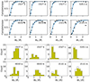 |
Fig. 2. Rest-frame equivalent width distributions. Upper panels: Completeness of W0 and exponential fit. W0 ≳ 2 Å produces blended doublet lines and are not used in the fit. Lower panels: Measured and completeness-corrected W0 distributions (filled and unfilled histograms, respectively). We note that system G311 a has a different y-scale. |
4. Spatial information and de-lensing
Clearly the most innovative – and we assert most powerful – feature of the present data set is its spatial coherence and resolution. In the so-called image plane (Grossman & Narayan 1988), that is, the geometry recorded by the instrument, the present binned spaxels are non-overlapping squares (of 0 6 on a side); however, arcs are a consequence of strong lensing, so the observed spaxels do not represent the real geometry of the so-called absorber plane at zabs (Lopez et al. 2018). To reconstruct the absorber plane, we used parametric lens models built for each field using LenstoolTool (Jullo et al. 2007) and based on available HST imaging (for details, we refer the reader to the respective publications indicated in Table 1). We used these models to calculate the deflection angles and reconstruct the observed spaxel grid at the absorber plane by applying the lens equation to the spaxel vertices. The center of a spaxel in the absorber plane was taken to be the center of a spaxel in the image plane de-lensed back to the absorber plane.
Columns (3)–(5) of Fig. 1 show 2″ × 2″ stamps of the reconstructed absorber plane at each system’s redshift. Displayed are maps of W0, v, and absorption spread. As in column (2), these maps consist of detections only, except for the triangles, which indicate W0 ≤ 0.2 (2-σ) upper limits. This threshold roughly corresponds to a 50% W0-completeness on average. The W0 maps suggest spatial coherence on ∼10 kpc scales down to W0 ≈ 0.3 Å.
The figure highlights the great advantage of the present data to reach down to sub-kiloparsec resolution at z ≈ 2. This is due basically to the absorber redshift being close to zsource, where beam separations approach zero. The drawback is that in some fields, the de-lensing produces heavily distorted grids, due to high magnification close to critical curves. There is also some level of overlapping spaxels, and in some cases their vertices even appear flipped. Both effects are nonphysical and likely reflect the spatial inaccuracy of the lens model at high magnifications. In this paper, we use average separations between spaxel centers and average spaxel areas only; we neglect the shape of the reconstructed spaxels.
The median spaxel area of C IV detections was found to be = 0.65 kpc2, so the median linear scale is ∼0.81 kpc. By system, the spaxel areas range from 0.5 to 3.6 kpc2. The total areas per system surveyed are small compared with strong C IV “sizes” of ∼100 kpc (linear) obtained with different methods (Rauch et al. 2001a; Steidel et al. 2010; Martin et al. 2010; Rudie et al. 2019; Hasan et al. 2022).
5. Line-of-sight versus transverse velocity dispersion
For each system, we defined two velocity dispersions: (1) a “transverse dispersion,” σ⊥, computed as the standard deviation of v of all spaxels along the arc (i.e., analogous to the projected velocity dispersion of galaxy clusters); and (2) a “parallel dispersion” (also “absorption spread”), defined as  , where σinst = σinst(λ) is the instrument spectral resolution (Table 3).
Ancillary data.
Figure 3 shows the distributions of v and σ∥ (blue and yellow histograms respectively). The vertical dashed lines indicate the median v and median σ∥ (≡⟨σ∥⟩) Each system’s σ⊥ is indicated by the length of the blue horizontal line. One feature that stands out is that ⟨σ∥⟩> σ⊥ in all systems, despite the fact that both dispersions vary across systems. Also, the velocity histograms are roughly symmetric. This suggests some level of Gaussianity and little contamination by line-of-sight outliers.
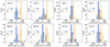 |
Fig. 3. Distribution of C IV doublet velocity (v) and absorption spread (σ∥) by system. The blue dashed line marks the zero-point velocity, and the orange dashed line indicates the median absorption spread (⟨σ∥⟩). The blue horizontal solid line has a size equal to the transverse velocity dispersion (σ⊥); its blue side is arbitrarily placed at zero velocity for a visual comparison between σ⊥ and ⟨σ∥⟩. The data represented in this figure has not been corrected for incompleteness. |
The measured σ⊥ could be biased high due to velocity outliers. On the other hand, sample incompleteness affects the low-W0 end, and since W0 and σ∥ are correlated by the Gaussian line fitting, ⟨σ∥⟩ may also be overestimated. To carry out a more robust comparison (system-by-system) between transverse and line-of-sight dispersions, we bootstrapped each sample by creating 1000 synthetic realizations of velocities and dispersions. These are drawn randomly from  and
and  , where v, σ∥, and their respective variances correspond to the measured values. From the bootstrapped distributions per system, we took the median and standard deviations as corrected values. A Monte Carlo (MC) analysis (Appendix D) showed that the S/N selection function introduces a spurious dispersion of ≈17–29 km s−1 (system dependent) in the spatial direction. This value was subtracted in quadrature, although it has only a marginal effect on σ⊥. As for ⟨σ∥⟩, the same MC analysis showed that our survey misses ≲10% of the systems detectable with MUSE (up to ∼30% in 2111 a and 2111 b). It is hard to assess the effect of this bias on ⟨σ∥⟩, but it would translate into a less than 5% only upward bias in the “worst-case” scenario that all missed systems have σ∥ ≈ 0 km s−1.
Figure 4 shows the median absorption spread by system, ⟨σ∥⟩ as a function of σ⊥ with corresponding 1σ errors. We observed that ⟨σ∥⟩> σ⊥ remains, and we note that it cannot be induced by the corrections described above. The relative spaxel areas probed by each system (circle sizes) do not seem to correlate with any of the above measurements (nor the total areas probed). Conversely, the median W0 broadly correlates with ⟨σ∥⟩, but this is expected based on the former results from fitting the velocity spread.
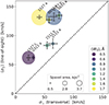 |
Fig. 4. System-by-system median absorption spread versus transverse velocity dispersion. Errors result from a bootstrapping analysis (Sect. 5). Circle areas are proportional to the absorber-plane mean spaxel area (in square kiloparsecs), and colors indicate the median rest-frame equivalent width per system (in Å). σ∥ has been corrected for the instrumental profile width (Sect. 5), and σ⊥ has been corrected for the spurious dispersion induced by each system’s S/N selection function (Appendix D). |
6. Transverse auto-correlation of velocities
Whilst the simple comparison between σ∥ and σ⊥ can have profound implications on the origin of the enriched gas and its kiloparsec-scale substructure, it is sensitive to outliers and hard to interpret. In this section, we use a more sophisticated statistical tool by measuring coherence in pairwise velocity differences and separations. To this end, we defined a transverse velocity auto-correlation function, computed it on a system-by-system basis, and tested the possibility that this function (1) unveils the spatial structure and (2) is related to the line-of-sight velocity correlation measured in quasar spectra (e.g., Steidel 1990; Petitjean & Bergeron 1994; Pichon et al. 2003; Scannapieco et al. 2006; Boksenberg & Sargent 2015; Rauch et al. 1996; Fathivavsari et al. 2013).
6.1. Definition
We defined a transverse velocity auto-correlation function, ξ(Δr⊥, Δv), as the excess probability of finding a given pairwise C IV absolute velocity difference, |Δv|, and we binned the spaxel separation on the reconstructed absorber plane, Δr⊥. We used the so-called natural estimator (e.g., Kerscher et al. 2000):
 (1)
(1)
where ⟨DD⟩ and ⟨RR⟩ are data-data and random-random pair averages, respectively. The pairs were created from data and random catalogs described below. To account for errors in ξ(Δr⊥, Δv), measured velocities were randomized with standard deviation δv, and ⟨DD⟩ was computed from the median values in the (Δr⊥, Δv) bin. The 1-σ errors result from adding in quadrature the standard deviation of the median statistics (“measurement” noise) with the square root of the number of data pairs (“shot” noise). See Appendix F.1 for more details.
6.2. Data catalogs
Each system’s data catalog consists of entries of (1) a C IV sight line de-lensed RA-DEC coordinate; (2) a rest-frame equivalent width W0 and its 1σ error, δW; (3) a velocity v and its 1σ error, δv; and (4) the same continuum S/N level used to pre-select spaxels. Data catalogs were used to create a list of pairwise velocity differences, |Δv|, and separations on the sky, Δr⊥. We assumed that the absorption signal is spatially independent from one spaxel to another.
6.3. Random catalogs
Random catalogs must account for each system’s S/N selection function (e.g., Tejos et al. 2014), both in the spectral and transverse directions. Here, we followed a similar procedure as in Martin et al. (2010) and Mintz et al. (2022), albeit with important differences due to our particular data type.
For each system, we first created a new catalog filled with five repeated copies of the data catalog (including non-detections). This has the advantage of preserving the survey geometry4. Each catalog entry was populated by a (RA-Decran,W0ran, vran)-triplet, where (1) coordinates are uniformly distributed within the sky patch defined by all pre-selected spaxels; (2) W0ran is drawn randomly from the completeness-corrected W0 distribution, with replacement – we did not use a model of the W0 distribution (e.g., Mintz et al. 2022) because its shape is unknown in arc data; and (3) vran is drawn randomly from a uniform distribution of velocities, ![Mathematical equation: $ {\cal U}_{[-4000,4000]} $](/articles/aa/full_html/2024/11/aa51200-24/aa51200-24-eq14.gif) , of spatially unresolved velocity components in the search window, which we consider the sample boundary (Mo et al. 1992). (See Appendix F.2 for more details on the third condition.) Entries were rejected if W0ran < 3 × δW, where δW = FWHM/⟨S/N⟩/(1 + z) is the detection limit set by the average S/N at the wavelength corresponding to vran. These entries become random non-detections. Otherwise, if accepted, the entries become random detections. In practice, the S/N is quite flat over the small wavelength range under consideration, implying that the final selection is determined mostly by the spaxel-to-spaxel S/N variations. Finally, RR pairs were built in exactly the same fashion as DD pairs. The fidelity of the random catalogs is tested in Appendix F.3 using mock catalogs of unclustered data.
, of spatially unresolved velocity components in the search window, which we consider the sample boundary (Mo et al. 1992). (See Appendix F.2 for more details on the third condition.) Entries were rejected if W0ran < 3 × δW, where δW = FWHM/⟨S/N⟩/(1 + z) is the detection limit set by the average S/N at the wavelength corresponding to vran. These entries become random non-detections. Otherwise, if accepted, the entries become random detections. In practice, the S/N is quite flat over the small wavelength range under consideration, implying that the final selection is determined mostly by the spaxel-to-spaxel S/N variations. Finally, RR pairs were built in exactly the same fashion as DD pairs. The fidelity of the random catalogs is tested in Appendix F.3 using mock catalogs of unclustered data.
6.4. Results
Figure 5 displays ξ(Δr⊥, Δv) computed for all eight systems. The arbitrary sampling in Δr⊥ and Δv minimizes the number of no-data bins while keeping enough S/N in the less populated bins. The signal indicates evident velocity clustering below ∼100 km s−1 in most systems. For the systems 1527 b and 0033 a, the velocity differences are more uniformly distributed. In general, no spatial correlation was observed. If present, either our “resolution element” (the total area per system) does not resolve it or the de-lensed coordinates are too uncertain over these scales.
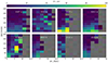 |
Fig. 5. C IV transverse velocity auto-correlation, ξ(Δr⊥, Δv). Gray colored bins indicate no data. |
Figure 6 shows the velocity projection of ξ(Δr⊥, Δv), hereafter ξarc(Δv), created through merging bins in the spatial direction. Errors include both the bootstrapping analysis and Poisson statistics but are dominated by the latter. Consistent with Fig. 5, a significant amount of power is seen below ∼100 km s−1. For some systems (1527 b, 0033 a and 0033 b), a similar amount of power is seen for velocity differences up to 200 km s−1. We note that none of these signals can be mimicked by measurement errors only (dashed lines), except perhaps for 1527 c. Remarkably, ξarc(Δv) exhibits a strong similarity – in shape and amplitude – to the velocity two-point correlation function measured along quasar sight lines (hereafter ξQSO(Δv)). This seems sensible because ξQSO(Δv) is measured for C IV “velocity components” in high-resolution (HR; R ∼ 40 000) spectra (Rauch et al. 1996; Scannapieco et al. 2006; Fathivavsari et al. 2013; Boksenberg & Sargent 2015) that our data cannot resolve. This similarity is this article’s main object of study.
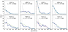 |
Fig. 6. Velocity projection of ξ(Δr⊥, Δv). Blue squares represent the arc data. The 1σ errors (in pink) include both the bootstrapping analysis and the Poisson statistics described in Sect. 6.3 but are dominated by the latter. Dashed curves indicate the signal produced by a velocity field distributed as |

7. Kinematic model
In this section we present a simple kinematic model that attempts to explain the results reported in Sect. 5 and Sect. 6. Subsequently, we show that this model provides testable clues on the kiloparsec-scale kinematic and spatial structure of the C IV gas.
7.1. Model setup
We propose an underlying population of sub-spaxel absorbing gas clumps (or “clouds”) that the ARCTOMO observations cannot resolve spatially but that nevertheless induce detectable absorption at the cloud velocity. In line with the lack of strong spatial structure seen in ξ(Δr⊥, Δv), we consider that the clouds are uniformly distributed on the sky and follow a normal distribution of projected velocities  on the spatial scales probed here. To statistically re-create the observations, we envisioned spaxels that sample N such clouds on average (Fig. 7). We did not make any assumption regarding the intrinsic position of the clouds along the line of sight.
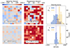 |
Fig. 7. Kinematic model with N = 4 (upper row) and N = 25 clouds sampled per spaxel. In both cases the underlying velocity field distributes as |

With this simplification, we computed the statistics of the sampled data, namely, (1) the distribution of the spaxel mean velocities and their dispersion, σ⊥, and (2) the distribution of the spaxel velocity dispersions, σ∥. Examples of (1) and (2) using σ0 = 100 km s−1 and two different values of N are shown in Fig. 7. Computing σ⊥ is exactly the same as measuring the velocity dispersion in an ARCTOMO system. Computing σ∥, on the other hand, is analogous to measuring the absorption dispersion in an ARCTOMO spectrum (but not exactly the same, as we are not dealing with absorption profiles). These definitions are based on the assumption that σ∥ conveys the kinematic information of individual velocity components in the real observations (i.e., “within” a spaxel). Hence, panels (a) and (b) in Fig. 7 are the model analog to the observations displayed in columns 4 and 5 of Fig. 1, respectively.
The histograms in Fig. 7 show the distributions of v and σ∥. They resemble the data histograms in Fig. 3. Indeed, a suit of model realizations shows that the larger the N, the narrower and more separated the two distributions become. For velocities (blue histograms), this is straightforward to see as the well-known consequence of spatial re-sampling, a process which ‘blurs’ the signal. In our case,
 (2)
(2)
On the other hand, for σ∥ (orange histograms), a large N not only narrows the distribution but it also shifts their peak to larger values. This effect is because, as more clouds are sampled per spaxel, their line-of-sight dispersions approach the original values of σ0. Thus, there must exist a relation also between the original dispersion, σ0, and the median line-of-sight dispersion, ⟨σ∥⟩. An analytic solution (Kenney & Keeping 1951) exists for the mean only, not the median of the σ∥ distribution. A good (within 1%) approximation for the median was found to be (Appendix F):
 (3)
(3)
As expected, the larger the number of clouds in a spaxel, the more the recovered dispersion approaches the original one. We note that the two equations above hold true independent of the physical spaxel size and depend only on N and σ0.
7.2. Model predictions
7.2.1. Transverse versus parallel velocity dispersion
Equations (2) and (3) show that the spatial sampling determines σ⊥ and ⟨σ∥⟩ and that this is a purely observational effect. Since we can measure σ⊥ and ⟨σ∥⟩ in ARCTOMO data, the equations can be used to derive two intrinsic properties of the cloud distribution, N and σ0. Solving for σ0, one obtains:
 (4)
(4)
from which we derive N, the per-spaxel mean number of clouds. In Table 4, N is listed for each system. Equation (4) can also be used to re-create Fig. 4 for particular values of N. This is shown in Fig. 8, where the white dashed lines display the ⟨σ∥⟩ versus σ⊥ relation for selected values of N. Since N does not need to be an integer, we interpreted it as the average number of clouds per spaxel. Equation (4) also explains why, under the assumption of Gaussianity, one should generally measure ⟨σ∥⟩> σ⊥ as a result of the particular ARCTOMO observations “flattening” the underlying velocity field5.
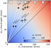 |
Fig. 8. Same as Fig. 4 but showing the two predictions of our kinematic model on (a) ⟨σ∥⟩ versus σ⊥ for a given number of clouds per spaxel, N (white dashed lines; Eq. (4)), and (b) the underlying line-of-sight dispersion, σ0 (background color; Eq. (5)). |
Model predictions.
Likewise, arranging Eqs. (2) and (3), this time to get rid of N, one finds
 (5)
(5)
Finally, an equation emerges that gives the underlying C IV velocity dispersion out of two ARCTOMO observables. The solutions for each system are listed in Table 4, and the background of Fig. 8 displays σ0 computed for all (σ⊥, ⟨σ∥⟩) combinations, as indicated by the color scale. The uncertainties in Table 4 were propagated from those in σ∥ and σ⊥. As a sanity check for Eq. (5), if σ⊥ = 0 (no transverse dispersion), then σ0 = ⟨σ∥⟩; that is, the underlying dispersion is recovered (and all spectra show the same centroid velocity). The second solution, σ0 = 0 (no absorption), is physical only for σ∥ = 0.
7.2.2. Inter-cloud distances
So far, our model does not involve physical scales, but we can define the (projected) mean number of clouds per unit area as ⟨Nc⟩≡N/Aspaxel, where Aspaxel is the mean spaxel area per system (hence, ⟨Nc⟩ is equivalent to the “counts-in-cylinder” statistics on galaxy scales; Berrier et al. 2011). With this definition, the projected mean distance between clouds is
![Mathematical equation: $$ \begin{aligned} \langle d_c^{2D} \rangle \sim \left(\frac{1}{\langle N_c \rangle }\right)^{1/2} \mathrm{[kpc].} \end{aligned} $$](/articles/aa/full_html/2024/11/aa51200-24/aa51200-24-eq22.gif) (6)
(6)
Using the values for ⟨Nc⟩ listed in Table 4, the present systems occur in structures separated on the sky by ⟨dc2D⟩ = 0.3–0.8 kpc. We discuss the implications of ⟨dc2D⟩ on cloud “sizes” in Sect. 7.2.3.
Likewise, ⟨Nc⟩ could constrain the number density of clouds nc = Nc/L, where L [kpc] is the (unknown) total absorption length. In this case, the mean 3D distance between clouds is
![Mathematical equation: $$ \begin{aligned} \langle d_c^{3D} \rangle \sim \frac{1}{n_c^{1/3}} \sim \left(\frac{L}{\langle N_c \rangle }\right)^{1/3} \mathrm{[kpc].} \end{aligned} $$](/articles/aa/full_html/2024/11/aa51200-24/aa51200-24-eq23.gif) (7)
(7)
From Table 4, we observed that the present systems arise in structures separated in space by ⟨dc3D⟩ = 2–4 (L/100)1/3 kpc. Current estimates on the extension of W0 ≳ 0.3 Å C IV halos amount to ≈100–200 kpc (Steidel et al. 2010; Hasan et al. 2022).
7.2.3. Cloud sizes and covering fraction
While our model does not constrain cloud “sizes” directly, our results suggest that cloud sizes cannot exceed the arc beams. In fact, if the clouds were much larger than the beam, we would measure (within observational uncertainties) the same velocity centroids across the entire arc and therefore also σ⊥ ≈ 0. As a result, ξarc(Δv) would be much steeper (given that Δv ≈ 0 across spaxels) than what we measure (Fig. 6). The only way to produce the observed signals at larger Δv is by having a cloud size that is about the same size or smaller than the spatial scale probed by a spaxel.
On the other hand, our model predicts a projected inter-cloud distance, ⟨dc2D⟩ (Eq. (6)). This parameter is related to the cloud characteristic size, Sc, and to the covering fraction, κ, defined as the fraction of the beam area covered by all clouds in projection along the line of sight. Our data cannot directly disentangle Sc and κ, but the following scenarios seem plausible:
-
κ ≈ 1, at the limit of no overlap: This implies cloud sizes of Sc ≈ ⟨dc2D⟩.
-
κ ≈ 1, with considerable overlap: This implies Sc ≳ ⟨dc2D⟩ but below the beam size for the reasons outlined above.
-
κ < 1: In this case, sizes remain unconstrained but below ⟨dc2D⟩.
Table 4 displays Sc = ⟨dc2D⟩ (first scenario, which we consider the most likely), using Eq. (6) and the tabulated ⟨Nc⟩ values. We emphasize that these considerations apply to clouds producing detectable ARCTOMO signals (i.e., typically W0 ≳ 0.3 Å).
In conclusion, our kinematic model constrains strong C IV cloud sizes to be of the order of or smaller than the probed beam size (i.e., ≲1 kpc). Future higher spatial and spectral resolution data should help discern between the scenarios described above.
7.2.4. Transverse auto-correlation
Our kinematic model can also predict ξarc(Δv) (Sect. 6.4). Recalling that if a random variable X is normally distributed with variance σ2, then ΔX is normally distributed, too (with variance 2σ2), Eq. (2) implies that
 (8)
(8)
where σξarc is the 1σ width of ξarc(Δv). The green curves in Fig. 6 compare this prediction with the measured ξarc(Δv). Since the model only predicts the width of ξarc(Δv), we display a Gaussian with an amplitude given by the maximum value of ξarc(Δv) and a width given by Eq. (8), using σ0 and N listed in Table 4 (a comparison between fitted and predicted widths is shown in Fig. F.2). The measurement and the prediction match reasonably well, which demonstrates the self-consistency of the model (since both quantities are based on the same data).
7.2.5. Prediction using the quasar line-of-sight correlation
As an independent test, our model can also predict ξarc(Δv) from ξQSO(Δv). To this end, we first stacked and averaged ξarc(Δv) over all eight systems. Next, we assumed that the C IV clouds abide to a normal distribution that is captured by both ξarc(Δv) and ξQSO(Δv); in other words, the clouds are responsible for both the parallel signal toward quasars and the transverse signal toward arcs. This is a strong assumption that we discuss further below in Sect. 8.1. From Eq. (8), it follows that  . Boksenberg & Sargent (2015) fit ξQSO(Δv) with the sum of two Gaussians having σξquasar = 80 and 185 km s−1 (also with a narrower one that our data do not resolve). Scannapieco et al. (2006) and Fathivavsari et al. (2013) do not provide fits, but their correlation functions have widths consistent with these. In Fig. 9, we display a comparison between our transverse correlation and the line-of-sight “QSO prediction” using N = 6.7, the weighted average number of clouds per spaxel in the arc data. The match is quite good (≲2σ deviation), lending independent support to our kinematic model and to the inferred number of clouds per spaxel. It also suggests that the present (modest) number of C IV systems is only moderately affected by cosmic variance.
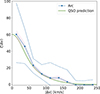 |
Fig. 9. Stacked average ξarc(Δv) of all eight arc systems and QSO prediction (details in Sect. 7.2.5). The dashed curves indicate the range of arc systems. |
8. Discussion
The proposed kinematic model seems acceptable on two different fronts: a self-consistent comparison between ARCTOMO transverse and line-of-sight kinematics, and a prediction of the transverse velocity auto-correlation from the quasar line-of-sight kinematics. The first one is solely observational, as we have outlined above. But the second suggests that the weak C IV components (only detected in HR quasar spectra) and the strong components (our arc detections) may trace the same physical structures. We conclude this article by discussing how our results are consistent with even more quasar observations and how together they provide glimpses of the CGM on both the sub-kiloparsec and galactic scales.
8.1. Cloud density structure
A natural explanation for a single cloud population giving rise to both strong and weak components is that each cloud has an internal density structure. Consequently, as a second-order approximation of the model, in the following we refer to cloud “cores” (the central parts of the clouds responsible for the strong components) and “halos” (external parts of the clouds responsible for the weak components).
Figure 10 illustrates the proposed situation. The left-hand panel displays a column-density “map” of cloud cores and halos. The white dot represents a narrow beam (e.g., a quasar beam), and the squares represent the arc beams (e.g., ARCTOMO spaxels). In this simple example, the beams pierce a clumpy medium represented by the superposition of just four clouds. The right-hand panels display the respective spectra. These result from spatially averaging the flux within the beam areas (see the figure caption for more details on the implementation). By model construction, the narrow beam collects the kinematic information of many clouds through intercepting mostly their larger cross-section cloud halos. Each cloud produces a velocity component in an HR spectrum (lower-right panel). Conversely, a LR spectrum of the wide beam recovers only an average velocity and a line-of-sight dispersion (σ∥), and it is dominated by a few cloud cores inside the beam (upper-right panels). As expected, ⟨σ∥⟩> σ⊥ (see the figure caption for how σ∥ and σ∥ are represented).
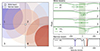 |
Fig. 10. Semi-schematic visualization of the kinematic model. Left-hand panel: Column density map, N(x). Here, x denotes the on-sky position. The map was created by superposing four clouds with |
A scenario of clouds producing both weak and strong components also explains why removing the high column-density components from quasar HR data does not affect ξQSO(Δv) (Scannapieco et al. 2006). Those authors find little change in ξQSO(Δv) when N = 1013, 14, 15 cm−2 components are excluded (up to 10% of their sample, according to the reported column density frequency). In the present interpretation, this effect is not simply due to the strong components being a small fraction of the total but more fundamentally to both strong and weak components sharing the same velocity field.
A cloud density structure equivalent to our model has already been proposed. For instance, Hummels et al. (2024) have introduced the concept of a cool CGM complex, which is composed of multiple cloudlets of various masses and velocities that lead to a column density structure, as in our case. However, we emphasize that our model aims to explain the observed kinematics only. Besides, the canonical one-to-one association between the cloud and the velocity component may also be too simplistic (e.g., Faerman & Werk 2023; Marra et al. 2024; Li et al. 2024).
8.2. Other multiple sight line observations
The most direct comparison between arc and quasar results can be made with the – unfortunately very limited – sample of multi-sight line quasar observations subtending approximately kiloparsec separations. The first direct estimate of C IV coherence length using lensed quasars (Rauch et al. 2001b) delivered ∼0.3 kpc (50% transverse variations). This value is consistent with subsequent studies that found C IV transverse structure below 1 kpc (Tzanavaris & Carswell 2003; Lopez et al. 2007; Rubin et al. 2018b). Along with the ten times larger ⟨dc3D⟩ computed in Sect. 7.2.2, the above narrow-beam size constraints imply a small volume filling factor of ∼10−3, which is in turn comparable with theoretical predictions (McCourt et al. 2018; Gronke & Oh 2020; Liang & Remming 2020; Li et al. 2024). On the other hand, combining those sizes with our ⟨dc2D⟩ constraint (Eq. (6)) leads to a near-unity covering fraction. This is again consistent with theoretical predictions (Liang & Remming 2020). We conclude that our arc results are consistent with quasar observations and theoretical predictions of the C IV spatial domain.
Regarding the line-of-sight direction, we measured ⟨σ∥⟩≈60–130 km s−1, a range which seems consistent with the velocity shear found toward lensed quasars. Rubin et al. (2018b) find a velocity structure Δv ≈ 100 km/s over kiloparsec scales; Rauch et al. (2001b) found ≈60 km s−1 over 10 kpc; Ellison et al. (2004) measured ≈15 km s−1 on sub-kiloparsec scales; and Lopez et al. (2007) found some cases with 60 km s−1 shear over 1 kpc. Thus, also in the parallel direction, arc and quasar observations seem consistent with each other.
8.3. Departures from Gaussianity and large-scale kinematics
Our model assumes an underlying Gaussian velocity field. In order to gauge departures from this idealization, we considered a spatial gradient in velocity, Δv, produced, for instance, by galaxy-scale motions such as orbiting, co-rotating, or out-flowing gas. Assuming the spatial scale of Δv is much larger than the spaxel size, it is straightforward to see that σ⊥ will increase but σ∥ will not. This is because the former is an inter-beam measurement, whereas the latter is an “intra-beam” one. In this case, Eq. (2) does not hold anymore, and in Fig. 4 all points become shifted to the right. A simple numerical test shows that N becomes underpredicted as soon as Δv is comparable to σ0. Thus, departures from Gaussianity could be detected in ARCTOMO systems exhibiting σ⊥ ≳ ⟨σ∥⟩ and ξ(Δr⊥, Δv) power both at large spatial and velocity scales. None of the present systems clearly qualifies in this group, but in principle our experiment could be used to identify large-scale kinematic motions of the absorbing CGM.
On the other hand, the large underlying velocity dispersions we derived are intriguing. The largest σ0 values in Table 4 suggest velocity dispersions of galaxy groups, and one possibility is that the unresolved clumps are bound to different group galaxies. Another one, of course, is that they feature the long-sought manifestation of super winds (Voit 1996; Pettini et al. 2001). Associations between C IV in quasar spectra and star-forming galaxies find kinematic separations at this level, and these have been associated with clustering (Adelberger et al. 2005; Lofthouse et al. 2023; Banerjee et al. 2023; Galbiati et al. 2023), inflows (Turner et al. 2017), or filaments outside the galaxy virial radius (Galbiati et al. 2023; Banerjee et al. 2023). All of these tests suggest that C IV in quasar spectra trace galaxies, although none of them really can disentangle the absorbing galaxy from the absorption system. Our transverse observations literally add a new dimension to the understanding of the origin of metal-rich gas in the z = 2–3 cool-warm CGM.
8.4. The path forward
It may seem surprising that the present ARCTOMO data, although unable to resolve the absorbing clouds neither spatially nor spectroscopically, still carry the 3D kinematic information encoded in their absorption profiles. We have shown that these data, along with simple assumptions about the kinematics, can lead to a set of realistic and testable predictions.
But the current tomographic data do not yet allow for a complete disentangling between different global dynamic models of the C IV-bearing CGM. The definitive pieces of the puzzle will be obtained through (1) the detection of the C IV galaxies responsible for the arc signals, a challenging objective that requires space-based near-infrared observations, and (2) spatially resolved HR observations of extended background sources, where little has been done yet (e.g., Diamond-Stanic et al. 2016). Along with more sophisticated models that include density structure, we assert that such observations shall dramatically improve our understanding of the cool-warm CGM’s small-scale structure. We consider, for instance, the HR curves in the upper-right panels of Fig. 10. If the kinematic model tested in this article is reliable, a small number of clouds per spatial resolution element of approximately kiloparsec size should unfold as resolved velocity components.
9. Summary
We have presented spatially resolved VLT/MUSE observations of four giant gravitational arcs that offer C IV coverage. We focused on the kinematic properties of C IV absorption detected at ⟨zabs⟩∼2.3, a redshift that enables sub-kiloparsec resolution of the absorbers thanks to lens magnification. Our experimental setup allowed us to analyze C IV absorption in 222 adjacent, uncorrelated beams that pierce eight intervening C IV systems. Our results are as follows:
-
Significant absorption is detected across almost all the arcs, implying C IV extensions (W0 ≳ 0.3 Å) of at least ≈10 kpc in the reconstructed absorber plane (Fig. 1). We ran an automated search of C IV absorption and computed doublet velocities, absorption spreads, and equivalent widths. Each system shows evident velocity clustering in the transverse direction (Fig. 3), and we set out to measure such clustering and investigated its origin.
-
On average, the transverse velocity dispersion, σ⊥, is found to be smaller than the per-system median line-of-sight dispersion, ⟨σ∥⟩ (Fig. 4).
-
To measure spatial clustering, we computed a transverse auto-correlation function of C IV velocities (ξ(Δr⊥, Δv); Fig. 5) and its velocity projection (ξarc(Δv); Fig. 6). ξ(Δr⊥, Δv) does not show evident spatial patterns, perhaps due to insufficient resolution. On the other hand, the average ξarc(Δv) exhibits great similarity in shape and amplitude with the line-of-sight two-point correlation measured in HR quasar spectra, ξQSO(Δv).
-
To aid a comparison between wide- (e.g., arc) and narrow- (e.g., quasar) beam observations, we introduced a simple kinematic model in which the absorption profiles result from groups of N clumps (clouds) sampled at the sub-spaxel level and that produce a mean velocity and line-of-sight dispersion (Fig. 7). The model successfully explains the σ⊥ < σ∥ inequality under the assumption of an underlying Gaussian field with dispersion σ0. It also consistently predicts N (Eq. (4)) and σ0 (Eq. (5)) out of the observables σ⊥ and σ∥ (Fig. 8). Combining this information with the average spaxel areas allowed us to constrain the number of clouds per unit area to within Nc ≈ 2–13 kpc−2 and σ0 ≈ 70–170 km s−1, depending on the system. The model also constrains the projected mean inter-cloud distance to within ≈0.3–0.8 kpc. The covering fraction and kinematic considerations put strong C IV sizes between those values and the spaxel size, 0.7–1.9 kpc.
-
Our model also predicts the width of ξarc(Δv) out of the independently computed ξQSO(Δv) reasonably well. Since ξQSO(Δv) is dominated by the bulk of weak velocity components that the arc data cannot resolve, this match led us to conclude that a single population of C IV clouds must be responsible for both signals. This in turn implies that the clouds must have a density structure, for instance, a radial density profile that produces a few strong components that shape ξarc(Δv) and many weak components that shape ξQSO(Δv) and only get detected in HR spectra (e.g., of quasars; Fig. 10). In such a scenario, ξQSO(Δv) is dominated by the weak components, as has been noted elsewhere.
-
We have discussed how our model and observations are compatible with extant observations of multiple quasars, both in the transverse and the parallel dimensions.
Upcoming large optical facilities will routinely enable tomography of the CGM using not only lensed galaxies but also normal galaxies. Comparison of these wide-beam observations with the extant narrow-beam statistics, as shown here for a handful of systems, promises a better understanding of the connection between the small- and the galactic-scale structure of the high-redshift CGM.
Data availability
Appendix A displaying the C IV spectra, corresponding line-profile fits, and best-fit parameters can be found in the Zenodo repository at https://zenodo.org/records/13891488
A gap between 5760–6010 Å is present due to the contamination produced by the sodium laser used in AO.
Velocity window chosen according to the correlation analysis explained in Sect. 6.
We did not bootstrap because replacement would bias the pairs toward zero separation.
Interestingly, ⟨σ∥⟩=σ⊥ for N = 1 + ϕ, where ϕ is the “Golden ratio.”
Acknowledgments
We would like to thank the anonymous referee for a thorough and critical review of our analysis. This work has benefited from discussions with Max Gronke, Joseph Hennawi, and Claudio Lopez. S. L. and N. T. acknowledge support by FONDECYT grant 1231187. M. S. was financially supported by Becas-ANID scholarship #21221511, and also acknowledges ANID BASAL project FB210003.
References
- Adelberger, K. L., Shapley, A. E., Steidel, C. C., et al. 2005, ApJ, 629, 636 [NASA ADS] [CrossRef] [Google Scholar]
- Afruni, A., Lopez, S., Anshul, P., et al. 2023, A&A, 680, A112 [NASA ADS] [CrossRef] [EDP Sciences] [Google Scholar]
- Bacon, R., Accardo, M., Adjali, L., et al. 2010, SPIE Conf. Ser., 7735, 773508 [Google Scholar]
- Banerjee, E., Muzahid, S., Schaye, J., Johnson, S. D., & Cantalupo, S. 2023, MNRAS, 524, 5148 [NASA ADS] [CrossRef] [Google Scholar]
- Becker, G. D., Pettini, M., Rafelski, M., et al. 2019, ApJ, 883, 163 [NASA ADS] [CrossRef] [Google Scholar]
- Berrier, H. D., Barton, E. J., Berrier, J. C., et al. 2011, ApJ, 726, 1 [NASA ADS] [CrossRef] [Google Scholar]
- Bird, S., Rubin, K. H. R., Suresh, J., & Hernquist, L. 2016, MNRAS, 462, 307 [NASA ADS] [CrossRef] [Google Scholar]
- Boksenberg, A., & Sargent, W. L. W. 2015, ApJS, 218, 7 [NASA ADS] [CrossRef] [Google Scholar]
- Bordoloi, R., Tumlinson, J., Werk, J. K., et al. 2014, ApJ, 796, 136 [NASA ADS] [CrossRef] [Google Scholar]
- Bordoloi, R., O’Meara, J. M., Sharon, K., et al. 2022, Nature, 606, 59 [NASA ADS] [CrossRef] [Google Scholar]
- Bordoloi, R., Simcoe, R. A., Matthee, J., et al. 2024, ApJ, 963, 28 [NASA ADS] [CrossRef] [Google Scholar]
- Cen, R., & Chisari, N. E. 2011, ApJ, 731, 11 [NASA ADS] [CrossRef] [Google Scholar]
- Chen, H.-W., Lanzetta, K. M., & Webb, J. K. 2001, ApJ, 556, 158 [NASA ADS] [CrossRef] [Google Scholar]
- Chen, H.-W., Gauthier, J.-R., Sharon, K., et al. 2014, MNRAS, 438, 1435 [NASA ADS] [CrossRef] [Google Scholar]
- Christensen, C. R., Davé, R., Governato, F., et al. 2016, ApJ, 824, 57 [CrossRef] [Google Scholar]
- Cooksey, K. L., Kao, M. M., Simcoe, R. A., O’Meara, J. M., & Prochaska, J. X. 2013, ApJ, 763, 37 [NASA ADS] [CrossRef] [Google Scholar]
- Cooper, T. J., Simcoe, R. A., Cooksey, K. L., et al. 2019, ApJ, 882, 77 [CrossRef] [Google Scholar]
- Coppolani, F., Petitjean, P., Stoehr, F., et al. 2006, MNRAS, 370, 1804 [NASA ADS] [CrossRef] [Google Scholar]
- Cowie, L. L., Songaila, A., Kim, T.-S., & Hu, E. M. 1995, AJ, 109, 1522 [NASA ADS] [CrossRef] [Google Scholar]
- Diamond-Stanic, A. M., Coil, A. L., Moustakas, J., et al. 2016, ApJ, 824, 24 [NASA ADS] [CrossRef] [Google Scholar]
- D’Odorico, V., Finlator, K., Cristiani, S., et al. 2022, MNRAS, 512, 2389 [CrossRef] [Google Scholar]
- D’Odorico, V., Bañados, E., Becker, G. D., et al. 2023, MNRAS, 523, 1399 [CrossRef] [Google Scholar]
- Dutta, R., Acebron, A., Fumagalli, M., et al. 2024, MNRAS, 528, 1895 [CrossRef] [Google Scholar]
- Ellison, S. L., Songaila, A., Schaye, J., & Pettini, M. 2000, AJ, 120, 1175 [NASA ADS] [CrossRef] [Google Scholar]
- Ellison, S. L., Ibata, R., Pettini, M., et al. 2004, A&A, 414, 79 [NASA ADS] [CrossRef] [EDP Sciences] [Google Scholar]
- ESO CPL Development Team 2015, Astrophysics Source Code Library [record ascl:1504.003] [Google Scholar]
- Faerman, Y., & Werk, J. K. 2023, ApJ, 956, 92 [NASA ADS] [CrossRef] [Google Scholar]
- Fathivavsari, H., Petitjean, P., Ledoux, C., et al. 2013, MNRAS, 435, 1727 [NASA ADS] [CrossRef] [Google Scholar]
- Faucher-Giguère, C.-A., & Oh, S. P. 2023, ARA&A, 61, 131 [CrossRef] [Google Scholar]
- Faucher-Giguère, C.-A., Kereš, D., & Ma, C.-P. 2011, MNRAS, 417, 2982 [CrossRef] [Google Scholar]
- Fernandez-Figueroa, A., Lopez, S., Tejos, N., et al. 2022, MNRAS, 517, 2214 [NASA ADS] [CrossRef] [Google Scholar]
- Fielding, D., Quataert, E., McCourt, M., & Thompson, T. A. 2017, MNRAS, 466, 3810 [NASA ADS] [CrossRef] [Google Scholar]
- Finlator, K., Doughty, C., Cai, Z., & Díaz, G. 2020, MNRAS, 493, 3223 [NASA ADS] [CrossRef] [Google Scholar]
- Fischer, T. C., Rigby, J. R., Mahler, G., et al. 2019, ApJ, 875, 102 [NASA ADS] [CrossRef] [Google Scholar]
- Galbiati, M., Fumagalli, M., Fossati, M., et al. 2023, MNRAS, 524, 3474 [NASA ADS] [CrossRef] [Google Scholar]
- Gontcho A Gontcho, S., Miralda-Escudé, J., Font-Ribera, A., et al. 2018, MNRAS, 480, 610 [NASA ADS] [CrossRef] [Google Scholar]
- Gronke, M., & Oh, S. P. 2020, MNRAS, 494, L27 [Google Scholar]
- Grossman, S. A., & Narayan, R. 1988, ApJ, 324, L37 [NASA ADS] [CrossRef] [Google Scholar]
- Hamilton, A. J. S., & Tegmark, M. 2004, MNRAS, 349, 115 [NASA ADS] [CrossRef] [Google Scholar]
- Hasan, F., Churchill, C. W., Stemock, B., et al. 2022, ApJ, 924, 12 [NASA ADS] [CrossRef] [Google Scholar]
- Hennawi, J. F., & Prochaska, J. X. 2007, ApJ, 655, 735 [NASA ADS] [CrossRef] [Google Scholar]
- Hennawi, J. F., Strauss, M. A., Oguri, M., et al. 2006, AJ, 131, 1 [Google Scholar]
- Hummels, C. B., Smith, B. D., Hopkins, P. F., et al. 2019, ApJ, 882, 156 [NASA ADS] [CrossRef] [Google Scholar]
- Hummels, C. B., Rubin, K. H. R., Schneider, E. E., & Fielding, D. B. 2024, ApJ, 972, 148 [NASA ADS] [CrossRef] [Google Scholar]
- Jullo, E., Kneib, J.-P., Limousin, M., et al. 2007, New J. Phys., 9, 447 [Google Scholar]
- Kenney, J. F., & Keeping, E. S. 1951, in Mathematics of statistics, ed. D. Van Nostrand (Princeton, N.J.) [Google Scholar]
- Kereš, D., Katz, N., Weinberg, D. H., & Davé, R. 2005, MNRAS, 363, 2 [Google Scholar]
- Kerscher, M., Szapudi, I., & Szalay, A. S. 2000, ApJ, 535, L13 [NASA ADS] [CrossRef] [Google Scholar]
- Krogager, J. K., Noterdaeme, P., O’Meara, J. M., et al. 2018, A&A, 619, A142 [NASA ADS] [CrossRef] [EDP Sciences] [Google Scholar]
- Kulkarni, V. P., Cashman, F. H., Lopez, S., et al. 2019, ApJ, 886, 83 [NASA ADS] [CrossRef] [Google Scholar]
- Ledoux, C., Noterdaeme, P., Petitjean, P., & Srianand, R. 2015, A&A, 580, A8 [NASA ADS] [CrossRef] [EDP Sciences] [Google Scholar]
- Li, Z., Gronke, M., & Steidel, C. C. 2024, MNRAS, 529, 444 [NASA ADS] [CrossRef] [Google Scholar]
- Liang, C., & Kravtsov, A. 2017, ArXiv e-prints [arXiv:1710.09852] [Google Scholar]
- Liang, C. J., & Remming, I. 2020, MNRAS, 491, 5056 [NASA ADS] [CrossRef] [Google Scholar]
- Lofthouse, E. K., Fumagalli, M., Fossati, M., et al. 2023, MNRAS, 518, 305 [Google Scholar]
- Lopez, S., Reimers, D., Gregg, M. D., et al. 2005, ApJ, 626, 767 [NASA ADS] [CrossRef] [Google Scholar]
- Lopez, S., Ellison, S., D’Odorico, S., & Kim, T.-S. 2007, A&A, 469, 61 [NASA ADS] [CrossRef] [EDP Sciences] [Google Scholar]
- Lopez, S., Tejos, N., Ledoux, C., et al. 2018, Nature, 554, 493 [NASA ADS] [CrossRef] [Google Scholar]
- Lopez, S., Tejos, N., Barrientos, L. F., et al. 2020, MNRAS, 491, 4442 [NASA ADS] [CrossRef] [Google Scholar]
- Maitra, S., Srianand, R., Petitjean, P., et al. 2019, MNRAS, 490, 3633 [NASA ADS] [CrossRef] [Google Scholar]
- Marra, R., Churchill, C. W., Kacprzak, G. G., et al. 2024, MNRAS, 527, 10522 [Google Scholar]
- Martin, C. L., Scannapieco, E., Ellison, S. L., et al. 2010, ApJ, 721, 174 [NASA ADS] [CrossRef] [Google Scholar]
- McCourt, M., Oh, S. P., O’Leary, R., & Madigan, A.-M. 2018, MNRAS, 473, 5407 [Google Scholar]
- McQuinn, M. 2016, ARA&A, 54, 313 [NASA ADS] [CrossRef] [Google Scholar]
- Mentz, J. J., La Barbera, F., Peletier, R. F., et al. 2016, MNRAS, 463, 2819 [Google Scholar]
- Mintz, A., Rafelski, M., Jorgenson, R. A., et al. 2022, AJ, 164, 51 [NASA ADS] [CrossRef] [Google Scholar]
- Mo, H. J., Jing, Y. P., & Boerner, G. 1992, ApJ, 392, 452 [NASA ADS] [CrossRef] [Google Scholar]
- Mortensen, K., Keerthi Vasan, G. C., Jones, T., et al. 2021, ApJ, 914, 92 [CrossRef] [Google Scholar]
- Nelson, D., Genel, S., Vogelsberger, M., et al. 2015, MNRAS, 448, 59 [Google Scholar]
- Noterdaeme, P., Srianand, R., & Mohan, V. 2010, MNRAS, 403, 906 [NASA ADS] [CrossRef] [Google Scholar]
- Oppenheimer, B. D., & Davé, R. 2006, MNRAS, 373, 1265 [NASA ADS] [CrossRef] [Google Scholar]
- Oppenheimer, B. D., & Davé, R. 2008, MNRAS, 387, 577 [NASA ADS] [CrossRef] [Google Scholar]
- Peeples, M. S., Corlies, L., Tumlinson, J., et al. 2019, ApJ, 873, 129 [Google Scholar]
- Péroux, C., Rahmani, H., Arrigoni Battaia, F., & Augustin, R. 2018, MNRAS, 479, L50 [Google Scholar]
- Petitjean, P., & Bergeron, J. 1994, A&A, 283, 759 [NASA ADS] [Google Scholar]
- Pettini, M., Shapley, A. E., Steidel, C. C., et al. 2001, ApJ, 554, 981 [NASA ADS] [CrossRef] [Google Scholar]
- Pichon, C., Scannapieco, E., Aracil, B., et al. 2003, ApJ, 597, L97 [NASA ADS] [CrossRef] [Google Scholar]
- Rahmati, A., Schaye, J., Crain, R. A., et al. 2016, MNRAS, 459, 310 [NASA ADS] [CrossRef] [Google Scholar]
- Rauch, M., Sargent, W. L. W., Womble, D. S., & Barlow, T. A. 1996, ApJ, 467, L5 [NASA ADS] [CrossRef] [Google Scholar]
- Rauch, M., Sargent, W. L. W., & Barlow, T. A. 1999, ApJ, 515, 500 [NASA ADS] [CrossRef] [Google Scholar]
- Rauch, M., Sargent, W. L. W., & Barlow, T. A. 2001a, ApJ, 554, 823 [NASA ADS] [CrossRef] [Google Scholar]
- Rauch, M., Sargent, W. L. W., Barlow, T. A., & Carswell, R. F. 2001b, ApJ, 562, 76 [NASA ADS] [CrossRef] [Google Scholar]
- Rubin, K. H. R., Diamond-Stanic, A. M., Coil, A. L., Crighton, N. H. M., & Stewart, K. R. 2018a, ApJ, 868, 142 [NASA ADS] [CrossRef] [Google Scholar]
- Rubin, K. H. R., O’Meara, J. M., Cooksey, K. L., et al. 2018b, ApJ, 859, 146 [NASA ADS] [CrossRef] [Google Scholar]
- Rudie, G. C., Steidel, C. C., Pettini, M., et al. 2019, ApJ, 885, 61 [NASA ADS] [CrossRef] [Google Scholar]
- Rupke, D. S., Veilleux, S., & Sanders, D. B. 2005, ApJS, 160, 115 [Google Scholar]
- Ryan-Weber, E. V., Pettini, M., & Madau, P. 2006, MNRAS, 371, L78 [NASA ADS] [CrossRef] [Google Scholar]
- Savitzky, A., & Golay, M. J. E. 1964, Anal. Chem., 36, 1627 [Google Scholar]
- Scannapieco, E., Pichon, C., Aracil, B., et al. 2006, MNRAS, 365, 615 [NASA ADS] [CrossRef] [Google Scholar]
- Schaye, J., Carswell, R. F., & Kim, T.-S. 2007, MNRAS, 379, 1169 [NASA ADS] [CrossRef] [Google Scholar]
- Sharon, K., Bayliss, M. B., Dahle, H., et al. 2020, ApJS, 247, 12 [CrossRef] [Google Scholar]
- Shen, S., Madau, P., Aguirre, A., et al. 2012, ApJ, 760, 50 [NASA ADS] [CrossRef] [Google Scholar]
- Simcoe, R. A., Sargent, W. L. W., & Rauch, M. 2004, ApJ, 606, 92 [Google Scholar]
- Songaila, A. 2005, AJ, 130, 1996 [NASA ADS] [CrossRef] [Google Scholar]
- Soto, K. T., Lilly, S. J., Bacon, R., Richard, J., & Conseil, S. 2016, MNRAS, 458, 3210 [Google Scholar]
- Steidel, C. C. 1990, ApJS, 72, 1 [NASA ADS] [CrossRef] [Google Scholar]
- Steidel, C. C., Erb, D. K., Shapley, A. E., et al. 2010, ApJ, 717, 289 [Google Scholar]
- Stern, J., Hennawi, J. F., Prochaska, J. X., & Werk, J. K. 2016, ApJ, 830, 87 [NASA ADS] [CrossRef] [Google Scholar]
- Tejos, N., Morris, S. L., Finn, C. W., et al. 2014, MNRAS, 437, 2017 [Google Scholar]
- Tejos, N., López, S., Ledoux, C., et al. 2021, MNRAS, 507, 663 [NASA ADS] [CrossRef] [Google Scholar]
- Theuns, T., Viel, M., Kay, S., et al. 2002, ApJ, 578, L5 [NASA ADS] [CrossRef] [Google Scholar]
- Turner, M. L., Schaye, J., Crain, R. A., et al. 2017, MNRAS, 471, 690 [NASA ADS] [CrossRef] [Google Scholar]
- Tytler, D., Gleed, M., Melis, C., et al. 2009, MNRAS, 392, 1539 [Google Scholar]
- Tzanavaris, P., & Carswell, R. F. 2003, MNRAS, 340, 937 [NASA ADS] [CrossRef] [Google Scholar]
- Vikas, S., Wood-Vasey, W. M., Lundgren, B., et al. 2013, ApJ, 768, 38 [NASA ADS] [CrossRef] [Google Scholar]
- Voit, G. M. 1996, ApJ, 465, 548 [NASA ADS] [CrossRef] [Google Scholar]
- Weilbacher, P. M., Palsa, R., Streicher, O., et al. 2020, A&A, 641, A28 [NASA ADS] [CrossRef] [EDP Sciences] [Google Scholar]
- Wiersma, R. P. C., Schaye, J., Dalla Vecchia, C., et al. 2010, MNRAS, 409, 132 [NASA ADS] [CrossRef] [Google Scholar]
- Zahedy, F. S., Chen, H.-W., Rauch, M., Wilson, M. L., & Zabludoff, A. 2016, MNRAS, 458, 2423 [NASA ADS] [CrossRef] [Google Scholar]
- Zahedy, F. S., Chen, H.-W., Johnson, S. D., et al. 2019, MNRAS, 484, 2257 [NASA ADS] [CrossRef] [Google Scholar]
Appendix B: On system identification and completeness
The C IV system identification runs over all masked spectra along the whole available redshift path and provides redshift candidates that feed the subsequent line profile fitting (described in Sect. 3.2). The algorithm employs Pearson correlation. To begin, whole-spectrum continua are estimated through iterative Savitzky-Golay filtering (Savitzky & Golay 1964). The identification is performed along every continuum-normalized spectral pixel having S/N> 4, wherein the observed flux is correlated with a template. The template is built as two inverted Gaussian profiles defined by the characteristic separation of the C IV doublet and the instrumental spectral resolution. High correlation (Pearson coefficient r > 0.7, typically) indicates a possible true doublet (Noterdaeme et al. 2010; Ledoux et al. 2015). The candidates are visually examined and classified as a C IV system if high correlation occurs in at least one binned spectrum. Eight systems are found (Table 2); notably, their W0 distributions reach such high values that these systems would have been easily discovered by eye. This suggests we are not missing systems of this kind. To roughly estimate the system completeness at the low-W0 end, we inject synthetic C IV doublets with properties zi and W0 and run the search in the vicinity of the i-pixel of each binned spectrum. We obtain on average ≈50% recovery wherein all spectra in a system have a doublet with W0 ∼ 0.7 Å.
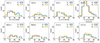 |
Fig. B.1. Distribution of errors in centroid velocity (δv) and absorption spread (δσ). |
Appendix C: Possible spatial sampling biases
To quantify spaxel-to-spaxel cross-talk effects, we performed two tests:
-
On the comparison between line-of-sight and transverse velocity dispersions (Sect. 5): we re-extracted and re-fit spectra using a larger aperture of
 -binned spaxels. Consistently, this decreases the number of spectra (by ∼40%) but should also counteract any possible cross-talk effects due to a FWHM
 PSF. The corresponding version of Fig. 4 shows broad consistency with the original one, that is, σ⊥ < σ∥ holds. Therefore, this test indicates that the inequality is not an artifact induced by the chosen
  aperture.
 -
On the transverse auto-correlation of velocities (Sect. 6): a 40% decrement in detections precludes the analysis of some of the systems due to their small number of pairs. Instead, to quantify the possible effect of
 apertures on ξ(Δr⊥, Δv) we recompute it excluding all neighbor spaxels in the image plane; that is, pairs made of information from adjacent binned spaxels are not considered. This exercise removes ∼10% of the sample pairs. Figure C.1 shows the results (for a better comparison we keep the mock and model curves as in Fig. 6). In all systems the correlation signal, although noisier, is preserved, indicating it is not driven by pairs of adjacent spaxels. Therefore, velocities measured using the
  aperture can be considered independent, that is, not biased by spaxel cross-talk effects. The exception is perhaps system 1527 c, whose correlation function is close to the signal expected from measurement errors only (indicated by the dashed lines in both figures). However, this system also shows the strongest overlapping effect in the reconstructed absorber plane, so ξ(Δr⊥, Δv) could be biased toward Δv = 0 km s−1 due to limitations of the lens model.
Appendix D: Spurious transverse dispersion
In Sect. 5 we compare σ⊥ and ⟨σ∥⟩. Naturally, we expect that low S/N spectra will lead to an increased scatter in the velocity uncertainties measured from Gaussian fitting, resulting in wider velocity distributions and thus higher σ⊥. In order to assess the magnitude of this systematic effect, we perform a MC re-sampling test. Each detected C IV doublet is ‘displaced’ to the same redshift, simulating a single-velocity distribution. This is achieved by replacing the originally fitted absorption lines with randomly selected flux from the adjacent pixels. After the doublet is essentially erased a double Gaussian profile is multiplied with the flux. These profiles have the same properties as the absorption features found in the data, for the corresponding spectra, except for the redshift which is set to the defined velocity center of the system. σ⊥ obtained from fitting these doublets (Table 3) should be purely due to each system’s S/N selection function.
Appendix E: Sample dispersion approximation
Equation (3) is obtained by trial and error on data produced by realizations of the model described in Sect. 7.1. Figure E.1 shows realizations for σ0 = 100 km s−1 and six different number of clouds per spaxel, N. Each of these realizations deliver a sample dispersion (⟨σ∥⟩) mean and median (blue and orange colors, respectively). The curves show solutions for the mean and the median (same respective colors). The exact solution for the mean is (Kenney & Keeping 1951):
 (E.1)
(E.1)
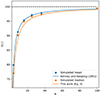 |
Fig. E.1. Mean and median sample dispersion versus number of scores per spaxel for σ0 = 100 km s−1. |
where Γ(n) is the complete gamma function. In this paper we use instead the approximation for the median given by Eq. (3).
Appendix F: On the velocity auto-correlation function
F.1. Error budget
To account for the variance of ξ(Δr⊥, Δv) due to uncertainties in the velocity measurements, σξ2(measurement), we ran 500 realizations of ξ(Δr⊥, Δv) by varying velocities according to  and computed the variance of the median statistics. On the other hand, the variance of ξ(Δr⊥, Δv) due to shot noise, σξ2(Poisson), was computed according to
 (F.1)
(F.1)
where DD (RR) is the number of data-data (random-random) pairs in a (Δr⊥, Δv) bin and NDD (NRR) is the total number of respective pairs.
The variance of ξ(Δr⊥, Δv) was taken to be the sum in quadrature of the above variances. This is dominated by σξ2(Poisson) due to both the small number statistics and the small velocity errors compared to the velocity bins (Figs. 5 and 6).
F.2. Random catalogs
Sampling a uniform distribution ![Mathematical equation: $ {\cal U}_{[a,b]} $](/articles/aa/full_html/2024/11/aa51200-24/aa51200-24-eq35.gif) (of variance
(of variance  ) results in a normal distribution of variance
  , where N is the number of averaged velocities. This implies that even a uniform velocity field will show velocity correlation if recorded with a beam that does not resolve the clouds spatially. Taking advantage of this property, we draw random ARCTOMO velocities from
  , where the random variance σRR2 = (8 0002/12)/N, that is, σRR2 is the binned variance of
 ![Mathematical equation: $ {\cal U}_{[-4000,4000]} $](/articles/aa/full_html/2024/11/aa51200-24/aa51200-24-eq39.gif) . For some systems we extend this range until convergence is achieved.
. For some systems we extend this range until convergence is achieved.
F.3. Mock catalogs
Despite the safeguards to account for each system’s complex selection function, some limitations remain: (1) random non-detections change the polygon edges (Hamilton & Tegmark 2004) and thus bias ξ close to the edges in the spatial direction; (2) individual data errors (both in velocity and spatially) can add spurious signal in ξ(Δr⊥, Δv).
To address these issues we build realistic mock catalogs by creating re-sized replicas of the data samples, exactly like in Sect. 6.3, but having a random uniform v in the range ( − 4 000, +4 000) km s−1, random RA-DEC normally distributed around spaxel centers with standard deviation 2.4 kpc (two de-lensed spaxels), and random W0 drawn from the quasar W0 distribution (Cooksey et al. 2013). As in Sect. 6.3, detections and non-detections are defined by confronting W0 with the detection limit set by the S/N. Each mock entry passes the same S/N criterion outlined above Fig. F.1 shows ξ(Δr⊥, Δv) measured for a mock data set, based on system 1527 a. As expected, there is no significant clustering power at any scale, which lends support to the technique and also to the fidelity of the random catalogs.
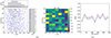 |
Fig. F.1. ξ(Δr⊥, Δv) measured for a realistic mock data set with no correlation. (a) In the scatter plot the blue (gray) dots correspond to the mock data (random) pairs, and the side panels show the respective projections in number counts. In the 2d-histogram the color scale indicates ξ(Δr⊥, Δv) between -1 and 1. (b) Velocity projection of ξ(Δr⊥, Δv). The shaded pink regions indicate 1σ errors. |
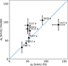 |
Fig. F.2. Per-system 1-σ width of ξarc(Δv) displayed in Fig. 6. This is computed via a single Gaussian fit of ξarc(Δv) (x-axis) or predicted by the kinematic model described by Eq. (8), using σ0 and N in Table 4 (y-axis). Error bars represent fit and propagated errors, respectively. |
On the other hand, to re-create the spurious signal that a single velocity across spaxels would produce, mock catalogs are created as above but having velocities distributed as  , where δv are the individual measurement errors. The dashed curves in Fig. 6 show the resulting ξ(Δr⊥, Δv).
All Tables
All Figures
|
Fig. 1. MUSE arc images and C IV system maps. Columns from left to right: Column (1): White-image stamps of the gravitational arcs. Column (2): |
| In the text | |
|
Fig. 2. Rest-frame equivalent width distributions. Upper panels: Completeness of W0 and exponential fit. W0 ≳ 2 Å produces blended doublet lines and are not used in the fit. Lower panels: Measured and completeness-corrected W0 distributions (filled and unfilled histograms, respectively). We note that system G311 a has a different y-scale. |
| In the text | |
|
Fig. 3. Distribution of C IV doublet velocity (v) and absorption spread (σ∥) by system. The blue dashed line marks the zero-point velocity, and the orange dashed line indicates the median absorption spread (⟨σ∥⟩). The blue horizontal solid line has a size equal to the transverse velocity dispersion (σ⊥); its blue side is arbitrarily placed at zero velocity for a visual comparison between σ⊥ and ⟨σ∥⟩. The data represented in this figure has not been corrected for incompleteness. |
| In the text | |
|
Fig. 4. System-by-system median absorption spread versus transverse velocity dispersion. Errors result from a bootstrapping analysis (Sect. 5). Circle areas are proportional to the absorber-plane mean spaxel area (in square kiloparsecs), and colors indicate the median rest-frame equivalent width per system (in Å). σ∥ has been corrected for the instrumental profile width (Sect. 5), and σ⊥ has been corrected for the spurious dispersion induced by each system’s S/N selection function (Appendix D). |
| In the text | |
|
Fig. 5. C IV transverse velocity auto-correlation, ξ(Δr⊥, Δv). Gray colored bins indicate no data. |
| In the text | |
|
Fig. 6. Velocity projection of ξ(Δr⊥, Δv). Blue squares represent the arc data. The 1σ errors (in pink) include both the bootstrapping analysis and the Poisson statistics described in Sect. 6.3 but are dominated by the latter. Dashed curves indicate the signal produced by a velocity field distributed as |
| In the text | |
|
Fig. 7. Kinematic model with N = 4 (upper row) and N = 25 clouds sampled per spaxel. In both cases the underlying velocity field distributes as |
| In the text | |
|
Fig. 8. Same as Fig. 4 but showing the two predictions of our kinematic model on (a) ⟨σ∥⟩ versus σ⊥ for a given number of clouds per spaxel, N (white dashed lines; Eq. (4)), and (b) the underlying line-of-sight dispersion, σ0 (background color; Eq. (5)). |
| In the text | |
|
Fig. 9. Stacked average ξarc(Δv) of all eight arc systems and QSO prediction (details in Sect. 7.2.5). The dashed curves indicate the range of arc systems. |
| In the text | |
|
Fig. 10. Semi-schematic visualization of the kinematic model. Left-hand panel: Column density map, N(x). Here, x denotes the on-sky position. The map was created by superposing four clouds with |
| In the text | |
|
Fig. B.1. Distribution of errors in centroid velocity (δv) and absorption spread (δσ). |
| In the text | |
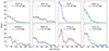 |
Fig. C.1. Same as Fig. 6 but excluding pairs by neighbor spaxels in the image plane. |
| In the text | |
|
Fig. E.1. Mean and median sample dispersion versus number of scores per spaxel for σ0 = 100 km s−1. |
| In the text | |
|
Fig. F.1. ξ(Δr⊥, Δv) measured for a realistic mock data set with no correlation. (a) In the scatter plot the blue (gray) dots correspond to the mock data (random) pairs, and the side panels show the respective projections in number counts. In the 2d-histogram the color scale indicates ξ(Δr⊥, Δv) between -1 and 1. (b) Velocity projection of ξ(Δr⊥, Δv). The shaded pink regions indicate 1σ errors. |
| In the text | |
|
Fig. F.2. Per-system 1-σ width of ξarc(Δv) displayed in Fig. 6. This is computed via a single Gaussian fit of ξarc(Δv) (x-axis) or predicted by the kinematic model described by Eq. (8), using σ0 and N in Table 4 (y-axis). Error bars represent fit and propagated errors, respectively. |
| In the text | |
Current usage metrics show cumulative count of Article Views (full-text article views including HTML views, PDF and ePub downloads, according to the available data) and Abstracts Views on Vision4Press platform.
Data correspond to usage on the plateform after 2015. The current usage metrics is available 48-96 hours after online publication and is updated daily on week days.
Initial download of the metrics may take a while.