| Issue |
A&A
Volume 691, November 2024
|
|
|---|---|---|
| Article Number | A263 | |
| Number of page(s) | 18 | |
| Section | Planets and planetary systems | |
| DOI | https://doi.org/10.1051/0004-6361/202451184 | |
| Published online | 18 November 2024 | |
Direct imaging and dynamical mass of a benchmark T-type brown dwarf companion to HD 167665★
1
Univ. Grenoble Alpes, CNRS, IPAG,
38000
Grenoble,
France
2
STAR Institute, Université de Liège,
Allée du Six Août 19c,
4000
Liège,
Belgium
3
Max-Planck-Institut für Astronomie,
Königstuhl 17,
69117
Heidelberg,
Germany
4
Department of Physics & Astronomy, Johns Hopkins University,
3400 N. Charles Street,
Baltimore,
MD
21218,
USA
5
Space Telescope Science Institute (STScI),
3700 San Martin Drive,
Baltimore,
MD
21218,
USA
6
INAF – Osservatorio Astronomico di Padova,
Vicolo dell’Osservatorio 5,
35122
Padova,
Italy
7
LESIA, Observatoire de Paris, Université PSL, CNRS, Sorbonne Université,
Université Paris Cité, 5 place Jules Janssen,
92195
Meudon,
France
8
European Southern Observatory (ESO),
Karl-Schwarzschild-Straße 2,
85748
Garching,
Germany
9
Université Lyon 1, ENS de Lyon, CNRS, Centre de Recherche Astrophysique de Lyon,
UMR5574,
69230,
Saint-Genis-Laval,
France
10
Observatoire de Genève, Université de Genève,
Chemin Pegasi 51,
1290
Versoix,
Switzerland
11
Institute for Astronomy, University of Edinburgh, Royal Observatory,
Edinburgh
EH9 3HJ,
UK
12
INAF – Osservatorio Astrofisico di Catania,
Via Santa Sofia 78,
95123
Catania,
Italy
13
Institutionen för astronomi, Stockholms universitet, AlbaNova universitetscentrum,
Roslagstullsbacken 21,
106 91
Stockholm,
Sweden
14
European Southern Observatory,
Alonso de Córdova 3107, Vitacura, Casilla
19001,
Santiago,
Chile
15
Instituto de Estudios Astrofísicos, Facultad de Ingeniería y Ciencias, Universidad Diego Portales,
Av. Ejército 441,
Santiago,
Chile
16
Millennium Nucleus on Young Exoplanets and their Moons (YEMS),
Santiago,
Chile
17
Aix-Marseille Univ., CNRS, CNES, LAM,
Marseille,
France
18
Institute of Astronomy, University of Cambridge,
Madingley Road,
Cambridge
CB3 0HA,
UK
19
Max Planck Institute for Extraterrestrial Physics,
Giessenbachstraße 1,
85748
Garching,
Germany
20
Leiden Observatory, Leiden University,
PO Box 9513,
2300 RA
Leiden,
The Netherlands
21
Center for Interdisciplinary Exploration and Research in Astrophysics (CIERA) and Department of Physics and Astronomy, North-western University,
Evanston,
IL
60208,
USA
22
Unidad Mixta Internacional Franco-Chilena de Astronomía CNRS/INSU UMI 3386 and Departamento de Astronomía, Universidad de Chile,
Casilla 36-D,
Santiago,
Chile
23
Astronomy Department, University of Michigan,
Ann Arbor,
MI
48109,
USA
24
University of Exeter,
Physics Building, Stocker Road,
Exeter
EX4 4QL,
UK
25
Universidade de Lisboa - Faculdade de Ciências,
Campo Grande,
1749-016
Lisboa,
Portugal
26
CENTRA - Centro de Astrofísica e Gravitação, IST, Universidade de Lisboa,
1049-001
Lisboa,
Portugal
27
Department of Astronomy, California Institute of Technology,
Pasadena,
CA
91125,
USA
28
Department of Astrophysical and Planetary Sciences, JILA,
Duane Physics Bldg., 2000 Colorado Ave, University of Colorado,
Boulder,
CO
80309,
USA
29
I. Institute of Physics, University of Cologne,
Zülpicher Straße 77,
50937
Cologne,
Germany
30
Max Planck Institute for Radio Astronomy,
Auf dem Hügel 69,
53121
Bonn,
Germany
31
Hamburger Sternwarte, Universität Hamburg,
Gojenbergsweg 112,
21029
Hamburg,
Germany
32
Universidade do Porto, Faculdade de Engenharia,
Rua Dr. Roberto Frias,
4200-465
Porto,
Portugal
33
School of Physics, University College Dublin,
Belfield,
Dublin 4,
Ireland
34
Academia Sinica, Institute of Astronomy and Astrophysics,
11F Astronomy-Mathematics Building, NTU/AS campus, No. 1, Section 4, Roosevelt Rd.,
Taipei
10617,
Taiwan
35
European Space Agency (ESA), ESA Office, STScI,
3700 San Martin Drive,
Baltimore,
MD
21218,
USA
36
ORIGINS Excellence Cluster,
Boltzmannstraße 2,
85748
Garching,
Germany
37
Max Planck Institute for Astrophysics,
Karl-Schwarzschild-Straße 1,
85748
Garching,
Germany
38
Departments of Physics and Astronomy, Le Conte Hall, University of California,
Berkeley,
CA
94720,
USA
39
Advanced Concepts Team, European Space Agency, TEC-SF, ESTEC,
Keplerlaan 1,
2201 AZ
Noordwijk,
The Netherlands
40
Department of Earth & Planetary Sciences, Johns Hopkins University,
Baltimore,
MD,
USA
★★ Corresponding author; annelisekatia.maire@gmail.com
Received:
19
June
2024
Accepted:
5
September
2024
Context. A low-mass companion potentially in the brown dwarf mass regime was discovered on a ~12 yr orbit (~5.5 au) around HD 167665 using radial velocity (RV) monitoring. Joint RV–astrometry analyses confirmed that HD 167665B is a brown dwarf with precisions on the measured mass of ~4–9%. Brown dwarf companions with measured mass and luminosity are valuable for testing formation and evolutionary models. However, its atmospheric properties and luminosity are still unconstrained, preventing detailed tests of evolutionary models.
Aims. We further characterize the HD 167665 system by measuring the luminosity and refining the mass of its companion and reassessing the stellar age.
Methods. We present new high-contrast imaging data of the star and of its close-in environment from SPHERE and GRAVITY, which we combined with RV data from CORALIE and HIRES and astrometry from HIPPARCOS and Gaia.
Results. The analysis of the host star properties indicates an age of 6.20 ± 1.13 Gyr. GRAVITY reveals a point source near the position predicted from a joint fit of RV data and HIPPARCOS–Gaia proper motion anomalies. Subsequent SPHERE imaging confirms the detection and reveals a faint point source of contrast of ∆H2 = 10.95 ± 0.33 mag at a projected angular separation of ~180 mas. A joint fit of the high-contrast imaging, RV, and HIPPARCOS intermediate astrometric data together with the Gaia astrometric parameters constrains the mass of HD 167665B to ~1.2%, 60.3 ± 0.7 MJ. The SPHERE colors and spectrum point to an early or mid-T brown dwarf of spectral type T4−2+1. Fitting the SPHERE spectrophotometry and GRAVITY spectrum with synthetic spectra suggests an effective temperature of ~1000–1150 K, a surface gravity of ~5.0–5.4 dex, and a bolometric luminosity log(L/L⊙)=−4.892−0.028+0.024 dex. The mass, luminosity, and age of the companion can only be reproduced within 3σ by the hybrid cloudy evolutionary models of Saumon & Marley (2008, ApJ, 689, 1327), whereas cloudless evolutionary models underpredict its luminosity.
Key words: methods: data analysis / techniques: high angular resolution / techniques: image processing / planets and satellites: dynamical evolution and stability / brown dwarfs / stars: individual: HD 167665
© The Authors 2024
 Open Access article, published by EDP Sciences, under the terms of the Creative Commons Attribution License (https://creativecommons.org/licenses/by/4.0), which permits unrestricted use, distribution, and reproduction in any medium, provided the original work is properly cited.
This article is published in open access under the Subscribe to Open model. Subscribe to A&A to support open access publication.
1 Introduction
Evolutionary models of brown dwarfs and giant exoplanets are commonly used to assess the mass of directly imaged companions to stars using the measured luminosity of the companion and age of the host star (e.g., Chabrier et al. 2000; Baraffe et al. 2003; Saumon & Marley 2008). Even so, these models remain poorly tested due to uncertainties in the atmospheric properties and the physics of the formation process (e.g., Marley et al. 2007; Marleau & Cumming 2014; Mordasini et al. 2017; Marleau et al. 2019) and the lack of companions with precisely measured mass, luminosity, and age (≲ 30%).
HD 167665 is a nearby field F9V star (Gray et al. 2006) located at a distance of 30.86 ± 0.09 pc (Gaia Collaboration 2016, 2021). Patel et al. (2007) reported the discovery of a potential brown dwarf companion on a ~12 yr and moderately eccentric orbit using radial velocity (RV) monitoring with the High Resolution Echelle Spectrometer (HIRES, Vogt et al. 1994). Their data cover almost a full orbit, which allowed them to infer good orbital and minimum mass constraints: period P = 4385 ± 64 d, eccentricity e = 0.337 ± 0.005, time at periastron passage T0 = 2 456 910 ± 70 JD, argument of periastron passage ω = 225.0 ± 1.1°, RV semi-amplitude κA = 609.8 ± 3.1 m s−1, and minimum mass M2 sin i = 50.3 ± 0.4 MJ. Sahlmann et al. (2011) monitored the star over almost a full orbit of the companion and confirmed its presence using the CORALIE spectrograph (Queloz et al. 2000). Their inferred orbital parameters and minimum mass mostly agree with those derived by Patel et al. (2007):  , e = 0.340 ± 0.005,
  JD (2014 November 26 UT), ω = 225.7 ± 0.9°, κA = 609.5 ± 3.3 m s−1, and M2 sin i = 50.6 ± 1.7 MJ.
Sahlmann et al. (2011) used astrometric data from HIPPARCOS (van Leeuwen 2007) jointly with their RV data to constrain the inclination and mass of the companion, but could not derive any constraints due to the low significance of the astrometric signature (<1 σ). Reffert & Quirrenbach (2011) also used the HIPPARCOS data of van Leeuwen (2007) to constrain the inclination and mass of the companion given the spectroscopic orbital parameters, and derived a 3σ upper mass limit of 137 MJ.
Recently, three studies confirmed the companion to have a mass in the brown dwarf regime, combining RV and astrometry (Feng et al. 2022; Barbato et al. 2023; Xiao et al. 2023). Only Feng et al. (2022) and Xiao et al. (2023) provide a mass estimate,  and
and  , respectively.
We present here direct imaging observations of the brown dwarf companion to HD 167665 and show that it is a cool T-type brown dwarf using the GRAVITY instrument (GRAVITY Collaboration 2017) at the Very Large Telescope Interferometer (VLTI) and the Spectro-Polarimetric High-contrast Exoplanet REsearch (SPHERE) instrument (Beuzit et al. 2019) at the VLT. The GRAVITY data were taken during the GRAVITY GTO program and the ExoGRAVITY large program (Lacour et al. 2020). The SPHE RE data were taken as part of the SpHere INfrared survey for Exoplanets (SHINE, Desidera et al. 2021; Langlois et al. 2021; Vigan et al. 2021). Furthermore, we used RV data of the star from CORALIE and HIRES as well as astrometric measurements of the star from HIPPARCOS and Gaia. We present an updated analysis of the properties of the host star in Sect. 2. We describe the imaging observations and the CORALIE RV data in Sect. 3. We fit the imaging, RV, and astrometric measurements simultaneously and derive orbital parameters and a dynamical mass for HD 167665B in Sect. 4. Sections 5 and 6 discuss the spectral properties of the companion and detection limits on putative additional companions in the system, respectively. We compare the dynamical and spectral properties of HD 167665B to model predictions in Sect. 7. We conclude in Sect. 8.
Stellar parameters of HD 167665.
2 Host star properties
The stellar properties of HD 167665 were considered in several studies in the literature, pointing toward a star slightly more massive and warmer than the Sun, with subsolar metallicity, not particularly young; there is some disagreement about evolution status and stellar age. We perform here an independent analysis, following the same methodology as in the studies of the host stars of other low-mass companions (e.g., Vigan et al. 2016; Peretti et al. 2019; Maire et al. 2020b).
In particular, we performed a spectroscopic analysis to infer the effective temperature Teff, gravity log 𝑔, and abundance of several elements. To this end, we considered a high signal-to-noise ratio (S/N) spectrum taken with CORALIE as part of the RV monitoring of the star (Barbato et al. 2023). This was analyzed using the q2 code by Ramírez et al. (2014) with the line list by Li & Ezzeddine (2023).
The resulting spectroscopic parameters are Teff = 6050 ± 74 K, log ?? = 4.06 ± 0.11 dex, microturbulent velocity ξ = 1.09 ± 0.06 km s−1, and iron abundance [Fe/H]= −0.14 ± 0.05 dex in the cooler and less metal-poor parts of the literature results (Table 1). To further constrain the stellar characteristics and have an appropriate reference for the benchmark brown dwarf companion, we also derived the abundances of several elements, as listed in Table 2. The abundance pattern is very close to solar ([X/Fe] ≈ 0 dex) for all species under scrutiny.
The stellar age was derived using the Bressan et al. (2012) stellar models exploiting the web interface PARAM (da Silva et al. 2006)1. When adopting our spectroscopic parameters with the nominal error bars, the resulting age is 6.20 ± 1.13 Gyr and the stellar mass M1 = 1.054 ± 0.032 M⊙. These error bars are the internal ones and do not include the systematic uncertainties of the models, which however are expected to be small thanks to the similarity of our target to the Sun.
We also inferred the lithium abundance by synthesizing the Li I doublet at 6707.78 Å. To accomplish this, we used the Python wrapper pymoogi2 of the code MOOG by Sneden (1973, 2019 version). The same model atmosphere employed for determining the abundance of iron and other elements was utilized; moreover, we adopted the line list that has been consistently used in our previous works. The resulting lithium abundance was determined to be A(Li)=2.46 ± 0.05 dex. This is slightly below the locus of the ~ 1.2 Gyr old open cluster NGC 752 (Boesgaard et al. 2022) and in the upper part of the distribution observed for the ~4 Gyr open cluster M67 (Jones et al. 1999; Pace et al. 2012).
The chromospheric activity is low, although with some scatter in the literature (log R′HK = −4.99 (Wright et al. 2004); log R′HK = −4.82 (Isaacson & Fischer 2010)) and the star is not detected in the ROSAT All Sky Survey. No rotation period determinations are available in the literature, except for the indirect ones from chromospheric emission, as expected considering the very low amplitudes of photometric modulations for late F-type stars at low activity levels.
Finally, the kinematic parameters are well within the distribution of thin-disk objects, as also suggested by the solar-scaled abundance pattern. However, the W velocity is incompatible with a young age (less than about 1 Gyr).
Considering the limited age sensitivity of lithium and activity after a few gigayears, we adopt the isochrone age. When comparing our analysis with previous analyses listed in Table 1, our analysis agrees with the scenario of a star with a mass close to solar and an age in the range ~5–7 Gyr, in line with the analyses of Luck (2017) and Llorente de Andrés et al. (2021). However, we acknowledge that several other literature analyses suggest a slightly more massive and younger star. All the age estimates in Table 1 are based on the method of model isochrones. The age and mass are inferred by interpolating a set of observables (e.g., our study based on the PARAM interface uses the Teff, [Fe/H], V mag, and parallax). The results of this method may thus be affected by the choice of the model isochrones, the set of observables used for the interpolation, and the estimated value of the observables. For the last point, higher Teff and/or [Fe/H] yield younger age and/or higher mass. Our age and mass estimates are likely due to our Teff estimate, which is in the low range of the literature values, although it agrees with the Gaia DR3 value listed in Table 1 (Gaia Collaboration 2023b). We could derive with PARAM an age of 3.6 Gyr and a mass of 1.12 M⊙, in line with the results of several other literature studies, by setting [Fe/H] to our upper limit and Teff to 6200 K, which is ~2σ higher than our estimate. In addition, we tested the choice of the set of observables by using the G-band photometry and BP-RP color in Gaia DR3 to interpolate the isochrones of Bressan et al. (2012) following the methodology described in Appendix E of Gaia Collaboration (2023a) and found a younger age and higher mass compared to our estimates in Table 1; we also assumed the same priors for the initial mass function for single stars and the stellar formation rate. Therefore, in the discussion of the properties of the brown dwarf companion (Sect. 7), we consider the scenario of a star with a mass close to solar and an age in the range ~5–7 Gyr as the main hypothesis for the stellar properties, but also discuss the impact of the alternate hypothesis of a slightly younger and more massive star.
Chemical abundances of HD 167665.
3 Observations and data analysis
3.1 SPHERE high-contrast imaging
HD 167665 was observed with SPHERE on UT 2021 May 20 (Table 3) in the standard IRDIFS mode, which allowed the simultaneous observations with the Infra-Red Dual-band Imager and Spectrograph IRDIS (Dohlen et al. 2008; Vigan et al. 2010) in the dual-band imaging mode with the H23 filter pair and the integral field spectrograph IFS (Claudi et al. 2008) in the YJ bands (spectral resolution R ~ 54). An apodized pupil Lyot coronagraph (Carbillet et al. 2011; Guerri et al. 2011; Martinez et al. 2009) was used.
To calibrate the flux of the images, we acquired unsaturated noncoronagraphic images of the star (hereafter reference point spread function or reference PSF) at the beginning and end of the sequence. To register the images, we also acquired coronagraphic images with four artificial crosswise replicas of the star (Langlois et al. 2013) at the beginning and end of the sequence. Nighttime sky background frames were taken and additional daytime calibration performed following the standard procedure at ESO.
The data were reduced with the SPHERE Data Center pipeline (Delorme et al. 2017a), which uses the Data Reduction and Handling software (v0.15.0, Pavlov et al. 2008) and custom routines. It corrected for the cosmetics and instrument distortion, registered the frames, and normalized their flux. For the IFS data (Mesa et al. 2015) it also calibrated them spectrally and extracted the image cubes. Subsequently, we sorted the frames using visual inspection to reject poor-quality frames (adaptive optics open loops, low-wind effect) and an automatic criterion to reject frames with low flux in the coronagraphic spot (semi-transparent mask). After this step we were left with 94% and 81% of the frames for the IRDIS and IFS data, respectively. Finally, the data were analyzed with a consortium image processing pipeline (Galicher et al. 2018). Figure 1 shows the images processed with angular differential imaging (ADI, Marois et al. 2006) with the principal component analysis algorithm (PCA, Soummer et al. 2012) provided in the consortium image processing pipeline. Five modes were used for the IRDIS data reduction and ten modes for the IFS data reduction. We also analyzed the data with alternative high-contrast imaging algorithms: Template Locally-Optimized Combination of Images (TLOCI, Marois et al. 2014), PAtch COvariances in angular and spectral differential imaging mode (PACO, Flasseur et al. 2018), Temporal Reference Analysis of Planets (TRAP, Samland et al. 2021), and ANgular DiffeRential Optimal Method Exoplanet Detection Algorithm (ANDROMEDA, Mugnier et al. 2009; Cantalloube et al. 2015). We compare the extracted spectrophotometry in Appendix A (see Fig. A.1).
The photometry and astrometry given in Tables 4 and 5 were measured in the PCA-reduced images using the negative fake planet injection approach (Galicher et al. 2018). The astrometry was calibrated following Maire et al. (2016), with pixel scales of 12.250 ± 0.009 mas/pix (H2) and 12.244 ± 0.009 mas/pix (H3) and a north correction angle of −1.76 ± 0.08º. The absolute magnitudes were computed using the 2MASS values (Cutri et al. 2003) for the stellar magnitudes. The IFS spectrum used in the spectral analysis (Sect. 5) was extracted in the PCA-reduced images. The variability of the PSF (~30%) is the main contributor to the error budget.
Observing log.
Photometry of HD 167665B.
Relative astrometry of HD 167665B.
3.2 GRAVITY dual-field data
HD 167665 was observed on UT 2021 March 3, 2021 August 27, and 2021 August 28 with GRAVITY in its dual-field mode combined with the four 8.2 m Unit Telescopes. The medium spectral resolution mode R ~ 500 was used. To position the GRAVITY science fiber for the first observation, which was obtained before the SPHERE observation (Sect. 3.1), we estimated the on-sky position of the companion using a joint fit of the RV data of Sahlmann et al. (2011) and HIPPARCOS–Gaia DR2 proper motion anomalies from Kervella et al. (2019) using the tool described in Maire et al. (2020a). For the subsequent GRAVITY observations, we predicted the on-sky position by including the SPHERE astrometry in the fit.
The GRAVITY data were reduced with a custom pipeline (Nowak et al. 2020). Figure 2 shows the resulting χ2 maps for the first two epochs. For the first displayed epoch, a clear signal is recovered at the predicted position. Its measured brightness is slightly fainter compared to the brightness of the companion predicted using evolutionary models given its measured mass and the system age estimated by Sahlmann et al. (2011), suggesting that HD 167665 is actually older (as shown in Sect. 2). The SPHERE imaging of the companion confirmed its faint-ness compared to the predictions and allowed for discriminating between the χ2 minima in the GRAVITY map.
The astrometric measurements for the first two epochs are given in Table 5. We checked for potential astrometric systematics between GRAVITY and SPHERE by interpolating the GRAVITY measurements at the SPHERE epoch. The SPHERE measurement is consistent with the GRAVITY astrometry within the SPHERE uncertainties. The GRAVITY spectrum used in the spectral forward modeling analysis (Sect. 5.2) is the weighted mean spectrum computed over the three data sets corrected for the fiber injection following Balmer et al. (2023), trimmed to the range 2.0–2.2 µm, and binned to a spectral resolution of~125.
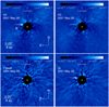 |
Fig. 1 SPHERE contrast images of HD 167665 (see text). The white arrows indicate the position of HD 167665B. The central regions of the images are numerically masked out to hide bright stellar residuals. The white cross in each panel indicates the location of the primary star. The contrast scales are the same between the IRDIS images (top row) and between the IFS images (bottom row). The companion appears significantly fainter in the H3 image because the spectral filter matches methane absorption bands, hinting that the companion is a T-type sub-stellar object. The images were smoothed using a Gaussian filter with a 2 pixel width. |
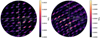 |
Fig. 2 GRAVITY χ2 maps of HD 167665 for epochs UT 2021 March 3 (left) and UT 2021 August 27 (right) centered on the pointed location on sky. The location of the companion is shown as a blue circle in each panel. The x- and y-axes are the offsets in RA and Dec with respect to the star. The field of view (dashed outer circles) corresponds to the fiber field of view (~60 mas). |
3.3 CORALIE RV data
HD 167665 has been observed since 1999 with the CORALIE spectrograph installed on the 1.2 m EULER Swiss telescope at La Silla observatory (Chile). Since its installation in 1998, CORALIE has undergone two upgrades (in 2007 and 2014, referenced hereafter as C07 and C14, respectively) that introduced small RV offsets that vary from star to star. The data obtained before JD epoch 2455260 were originally published in Sahlmann et al. (2011). The data obtained after this epoch were published in Barbato et al. (2023). The data were reduced in a homogeneous way.
4 Orbital fitting
We combined the CORALIE RV data with the HIRES RV measurements in Tal-Or et al. (2019), who corrected the measurements presented in Butler et al. (2017) for small systematics due to an instrument upgrade. The measurements are available through the VizieR interface. The HIRES and CORALIE data extend the RV time baseline to about two orbital periods (Fig. 3, top left panel).
For the astrometric data, we first checked the HIPPARCOS–Gaia EDR3 proper motion anomalies in the HIPPARCOS–Gaia catalog of accelerations (Brandt 2021): pmra_g_hg = −2.995 ± 0.129 mas yr−1 and pmdec_g_hg = −3.782 ± 0.090 mas yr−1 for Gaia (Gaia Collaboration 2021); pmra_h_hg = −2.869 ± 0.829 mas yr−1 and pmdec_h_hg = −3.981 ± 0.537 mas yr−1 for HIPPARCOS (Perryman et al. 1997; van Leeuwen 2007). These values imply an astrometric detection at (23.2, 42.3)σ with Gaia and (3.5, 7.4)σ with HIPPARCOS. The HIPPARCOS five-parameter solution describes well the measured motion (goodness of fit F2 of 0.94). The Gaia EDR3 five-parameter solution is weakly affected by the reflex motion (renormalized unit weight error RUWE of 1.804; Lindegren et al. 2021). The rate of multiple peaks in the Gaia EDR3 record is null, hence the data are not affected by flux contamination from another source. The star has no resolved common proper motion candidate companion in the Gaia EDR3 catalog (Kervella et al. 2022).
We ran an orbital fit using the BINARYS tool (orBIt determiNAtion with Absolute and Relative astrometrY and Spectroscopy, Leclerc et al. 2023). BINARYS can simultaneously adjust the residual abscissae from HIPPARCOS (in this study the Intermediate Astrometric Data, IAD, from van Leeuwen 2007), the astrometric parameters available from Gaia, relative astrometry, and RV. It uses a gradient descent method implementing automatic differentiation based on the R package TMB (Template Model Builder, Kristensen et al. 2016). The use of this approach is relevant for objects with well-constrained orbits, such as HD 167665B. The exploration of the uncertainties and degeneracies of the parameters is done by post-processing the TMB results with a short Markov chain Monte Carlo (MCMC) run using the R package tmbstan (Monnahan & Kristensen 2018). BINARYS implements a rigorous treatment of the information from HIPPARCOS and Gaia with minimal assumptions or simplifications. It adjusts the astrometric parameters (α, δ, ϖ, µα, µδ) in the HIPPARCOS reference frame at epoch J1991.25. The Gaia positions and proper motions are converted by taking into account the frame rotation between Gaia and HIPPARCOS and corrections for the Gaia EDR3 parallax and the parallax zero-point difference. The uncertainties on the five astrometric parameters are inflated according to the parallax error underestimation factor derived by El-Badry et al. (2021). The adjusted orbital parameters are (P, T0, a1, e, i, ω, Ω, a, γ), with a1 the semi-major axis of the orbit of the host star around the center of mass of the system, i the inclination, Ω the longitude of the ascending node, a the semi-major axis, and γ the systemic velocity. We present the results for Ω and ω relative to the orbit of the companion: ω is shifted by 180° compared to the values derived by Patel et al. (2007) and Sahlmann et al. (2011). The RV semi-amplitude is computed using the fitted parameters. The RV jitter is estimated using MCMC and kept fixed for the computation with TMB.
We excluded one outlier measurement in the HIPPARCOS IAD data (marked by its negative error on the residual abscissa). The RV reference for the zero-point (ZP) is C07. The first-guess solution used for the TMB computation includes information on the period (12 yr), the eccentricity (0.33), and the inclination (56º) based on a preliminary analysis using the approach of Maire et al. (2020a), and the RV semi-amplitude (609.5 m s−1) in Sahlmann et al. (2011). The global goodness of fit F2 is 0.8. The F2 value for the HIPPARCOS IAD is 0.96, which is similar to the published value (0.94, van Leeuwen 2007). Figure B.1, Fig. 3, and Table 6 summarize the results. The stellar mass inferred from the BINARYS analysis is in closer agreement with the alternate hypothesis of a slightly more massive star (Sect. 2).
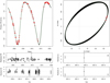 |
Fig. 3 Sample of 1000 model orbits fitted on the HD 167665B data (red points) from RV (top left) and imaging (top right) using the BINARYS tool (see text). The sample was drawn from 10 000 MCMC solutions (Appendix B). The solution derived by the TMB algorithm is shown as green dots. The RV and HIPPARCOS IAD residus (left, from middle to bottom) and the imaging residus (right, from middle to bottom) are computed with respect to the TMB solution. |
5 Spectral characterization
5.1 Empirical comparisons
First, we used the IRDIS dual-band photometry of the companion to compute the color–magnitude diagram in Fig. 4 (see details in Appendix C, and Appendix C of Bonnefoy et al. 2018). HD 167665B is located near mid-T template dwarfs and has a similar color to HD 13724B (Rickman et al. 2020) and HD 19467B (Crepp et al. 2014; Maire et al. 2020b).
Then, we used the SPHERE spectrum to carry out spectral typing with the SpeX spectral library available in the SPLAT toolkit (Burgasser 2014). We assess a spectral type of  . The best-match template spectrum is the spectrum of 2MASS J21513839-4853542, which is classified as T4 by Burgasser et al. (2006).
5.2 Forward modeling
Finally, we performed forward modeling of the SPHERE spectrophotometry and GRAVITY spectrum with atmospheric models. To convert the data from contrasts to physical fluxes, we used a model stellar spectrum and the instrument filter transmission curves. We fit a stellar spectrum from the BT-NextGen library (Allard et al. 2012) to measurements of the stellar spectral energy distribution (SED) available in the Virtual Observatory Sed Analyzer (Bayo et al. 2008) using nested sampling with the species library (Stolker et al. 2020). We used photometric data from Tycho (Høg et al. 2000), 2MASS (Cutri et al. 2003), and WISE (Cutri & et al. 2013), as well as Johnson photometry (Mermilliod 2006) and Strömgren photometry (Paunzen 2015). The surface gravity was kept fixed in the MCMC to the best-fit parameter found in Sect. 2. The metallicity was fixed to solar due to limitations in the parameter exploration in the model grid. Thus, we scaled the model spectrum to the data by adjusting the effective temperature, parallax, and radius. The effective temperature and parallax were allowed to vary within 3σ around their best estimate (derived in Sect. 2 and in Gaia EDR3, respectively). The radius was bound between 1 and 20 solar radii (R⊙). Inflated errors were enabled for the measured photometry, up to a factor of 20 for the optical measurements and up to a factor of 10 for the near-infrared measurements. A total of 500 live points were used. The model stellar spectrum was computed as the average of 100 random draws from the posterior distributions.
We fit the SED of HD 167665B with the atmospheric models BT-Settl (Allard et al. 2012), ATMO (Phillips et al. 2020), Sonora Bobcat (Marley et al. 2021), and the Morley et al. (2012) model using nested sampling with the species package. We chose these models from among the available models for their complementarity in parameter space and their extension to high surface gravities (>5 dex). The BT-Settl model assumes equilibrium chemistry and a nonparametric cloud model. The Sonora Bobcat model also assumes equilibrium chemistry, but no clouds. The ATMO NEQ strong model (hereafter ATMO SNEQ model) allows for testing the disequilibrium chemistry as an alternative process to clouds. The model of Morley et al. (2012) assumes equilibrium chemistry and a parametric cloud model (using a sedimentation parameter ƒsed, which increases for thinner clouds) and was developed to account for the condensation into clouds of chemical species in T- and Y-dwarf atmospheres other than iron and silicates (Cr, MnS, Na2S, ZnS, and KCl). The Sonora Bobcat models are the only models that explore the effects of the metallicity, which may be relevant considering that the star has been found to be subsolar (Table 1). We selected subgrids in effective temperature of the atmospheric models and, for the Sonora Bobcat models, in metallicity. The characteristics of the retained model grids are provided in Table 7. The radius of the companion (R2) was bound between 0.08 and 2 Jupiter radii (RJ). A Gaussian prior on the mass of HD 167665B was assumed, using the mass measured from the orbital fit (Table 6). A scaling factor for the SPHERE/IFS spectrum (aSPHERE_YJ) was used to account for potential systematics with respect to the GRAVITY spectrum and bound between 0.3 and 1.6. No weights were applied to the measurements. A total of 1000 live points were used.
Figures 5–8 show the posterior distributions of the parameters and the data compared to 30 fitted model spectra randomly drawn from the posterior distributions and degraded to a spectral resolution of 500. The derived atmospheric parameters are provided in Table 8. All models provide a reasonable fit to the SPHERE data given the large uncertainties. A higher dispersion is seen for the GRAVITY data, but still within 3σ for the most discrepant measurements. All models tend to predict a lower flux in the SPHERE/IRDIS H2 photometric band compared to the measured flux, but still within the large uncertainty except for the models of Morley et al. (2012). The effective temperatures inferred using all models are in the range ~ 1000–1200 K; the BT-Settl models and the Morley et al. (2012) models predict colder temperatures with respect to the ATMO SNEQ and Sonora Bobcat models. The posterior distributions for the surface gravity inferred using the ATMO SNEQ and Sonora Bobcat models reach the upper bound allowed in the grids, whereas the BT-Settl models predict a range of ~5.0–5.2 dex and the models of Morley et al. (2012) a range of ~4.9–5.2 dex. The radii predicted by the ATMO SNEQ and Sonora Bobcat models are in the range ~0.8–1.1 RJ, whereas the radii predicted by the BT-Settl models and the models of Morley et al. (2012) are larger with a range of 1.0–1.3 RJ. An upscaling for the SPHERE spectrometry by ~ 15–20% may be needed to fit all the models except for the models of Morley et al. (2012). The fit with the Morley et al. (2012) models requires a downscaling of ~30%. For all models, strong correlations are seen between the effective temperature, surface gravity, and radius, with smaller radii associated with higher surface gravities and effective temperatures. The bolometric luminosities predicted by all models are comprised between about −4.8 dex and −5.0 dex; the BT-Settl models predict the highest luminosity and the Morley et al. (2012) models predict the lowest luminosity. The fit with the Sonora Bobcat models provides loose constraints on the metallicity. The sedimentation parameter for the clouds in the models of Morley et al. (2012) is loosely constrained with a range of ~2.5–4.5.
To analyze the relative impact of the data sets on the atmospheric fits, we also carried out fits with the SPHERE and GRAVITY data separately (results not shown). In summary, the fits with the ATMO SNEQ, Sonora Bobcat, and Morley et al. (2012) models are robust against the used subset of the SPHERE+GRAVITY data, except for the bolometric luminosity log(L/L⊙), which is more driven by the GRAVITY data. The fits with the BT-Settl models provide parameters that differ by more than 1σ depending on the used subset of the SPHERE+GRAVITY data (>2.3σ between the SPHERE and GRAVITY fits, but <2σ between the GRAVITY and joint fits and <2.3σ between the SPHERE and joint fits), and the parameters inferred from the joint fit are between those inferred from the separate fits. The bolometric luminosity inferred using only the SPHERE data is lower than the value inferred from the GRAVITY data by ~ 1.5–3.2σ for all models except for the models of Morley et al. (2012), for which it is higher by ~2.5σ. The bolometric luminosity log(L/L⊙) inferred using only the SPHERE data differs from the bolometric luminosity log(L/L⊙) inferred from the joint fit by approximately −0.09 dex (2.3 σ) for the BT-Settl models, approximately −0.05 dex (1.4σ) for the ATMO SNEQ models, approximately −0.04 dex (1.2σ) for the Sonora Bobcat models, and ~0.12 dex (2.5σ) for the Morley et al. (2012) models.
Orbital parameters and dynamical mass of HD 167665B derived using the BINARYS tool.
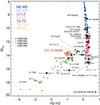 |
Fig. 4 Color-magnitude diagram of HD 167665B (red) using the IRDIS photometry. Template dwarfs (colored points) and a few young low-mass companions (black labels) are also shown for comparison. |
Characteristics of the atmospheric model grids adjusted on the spectral energy distribution of HD 167665B (see text).
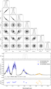 |
Fig. 5 Atmospheric fitting of HD 167665B with BT-Settl models. Top: corner plot of the retrieved parameters: Teff, log ɡ, radius, parallax, SPHERE/IFS scaling factor, log(L/L⊙), and mass. Bottom: comparison of the best-fit model spectra (black and gray) and photometry (open blue squares) with the measured SED (filled data points). The black model spectrum corresponds to the best-fit solution, whereas the gray model spectra were randomly drawn from the posterior distributions. The fit residuals are shown in the bottom panel and the filter transmission curves of SPHERE/IRDIS in the top panel. |
Atmospheric parameters derived for HD 167665B.
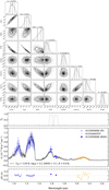 |
Fig. 7 Same as Fig. 5, but for Sonora Bobcat models. The retrieved parameters in the corner plot are Teff, log ɡ, [M/H], radius, parallax, SPHERE/IFS scaling factor, log(L/L⊙), and mass. |
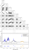 |
Fig. 8 Same as Fig. 5, but for the Morley et al. (2012) models. The retrieved parameters in the corner plot are Teff, log ɡ, ƒsed, radius, parallax, SPHERE/IFS scaling factor, log(L/L⊙), and mass. |
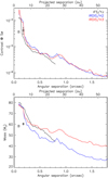 |
Fig. 9 SPHERE 5σ detection limits for contrast with respect to the star (top) and for mass (bottom) on putative additional companions around HD 167665 (see text). We also indicate the location of the companion for comparison (contrast in the H2 filter used in the contrast panel). |
6 Detection limits
Figure 9 shows the SPHERE detection limits at 5σ for contrast with respect to the star and for companion masses. For the contrast to companion mass conversion, we assumed the evolutionary model COND (Baraffe et al. 2003) with the atmospheric models of Baraffe et al. (2015) and a system age of 6 Gyr. The detection limits account for the coronagraphic transmission (Boccaletti et al. 2018) and the small sample statistics correction (Mawet et al. 2014). The detection limit in companion mass in the H3 filter is shallower than the curve for the H2 filter at separations beyond 0.2″ because the H3 magnitudes are dimmed by methane absorption bands. We can exclude additional companions more massive than ~47 MJ beyond 0.5″ (~15 au) and ~40 MJ beyond 1″ (~31 au). HD 167665B lies on the IRDIS contrast curve in the H2 filter, while it lies below the corresponding mass curve. As discussed in Sect. 7, the COND evolutionary model predicts higher masses for the measured luminosity and age of the brown dwarf with respect to its measured mass. A younger system age (Sect. 2) would shift the detection limits for companion mass predicted by the COND model toward lower values and the mass predicted for HD 167665B in closer agreement with the dynamical mass.
Barbato et al. (2023) present minimum mass detection limits based on RV data on putative additional companions around HD 167665 and exclude at 100% companions more massive than 0.9 MJ interior to HD 167665B assuming the same orbital inclination. This is significantly deeper compared to our imaging detection limits. Our imaging limits improve upon the RV detection limits for separations beyond ~60 au (outside the range shown in Fig. 9).
7 Discussion
Evolutionary models
Figure 10 shows the effective temperature and bolometric luminosity as a function of age predicted by several evolutionary models (colored points with uncertainties) assuming the 68.3% confidence interval for the companion mass from the orbital fit (Table 6): the cloudless COND model (Baraffe et al. 2003), the cloudless and hybrid cloudy models of Saumon & Marley (2008), and the cloudless model of Burrows et al. (1997). The hybrid cloudy model of Saumon & Marley (2008) models the disappearance of the clouds at the L/T transition (Teff ~ 1200–1400 K) by increasing the cloud sedimentation parameter with decreasing Teff. The evolutionary model is computed assuming for the atmospheric model a combination of cloudless and cloudy atmospheric models. We refer to Saumon & Marley (2008) for a detailed discussion of the differences between their models and the COND and Burrows et al. (1997) models. Briefly, the cloudless model of Saumon & Marley (2008) uses a different atmospheric model for the surface boundary condition and does not include the electron conduction in the core of the object compared to the COND model. The latter effect produces lower luminosities. The models of Burrows et al. (1997) assume a lower value for the helium abundance (0.25 vs. 0.28 dex) and a less opaque atmosphere compared to the cloudless model of Saumon & Marley (2008). Both effects result in lower luminosities. We could not use the evolutionary tracks of Baraffe et al. (2015) because they do not extend to effective temperatures below ~1400 K at the age range of the target.
To discuss the surface gravity of HD 167665B, we show in Fig. 11 the surface gravity as a function of the effective temperature predicted for several ages and companion masses by the hybrid cloudy models of Saumon & Marley (2008). Similar conclusions are reached when using the other evolutionary models used in Fig. 10.
We first discuss the individual estimates for the effective temperatures, surface gravities, and bolometric luminosities derived for all atmospheric models in Table 8 with respect to the predictions of the evolutionary models. The 1σ regions for the effective temperature and surface gravity are shown as colored rectangles in Fig. 11. The effective temperatures are coherent with the expectations given the age and mass constraints (~ 1000–1150 K, top panel of Fig. 10 and Fig. 11). The surface gravities fitted with all atmospheric models except for the BT-Settl models would be compatible with the predictions of evolutionary models (~5.3–5.4 dex, Fig. 11), whereas the surface gravity derived for the BT-Settl models is lower by ~2σ. The bolometric luminosities predicted by all atmospheric models are higher by more than 3tr than the expectations of cloudless evolutionary models (from about −5.3 to −5.1 dex, bottom panel of Fig. 10). The predicted bolometric luminosities of the hybrid cloudy evolutionary model of Saumon & Marley (2008) would provide a better match to the measured values for ages close to the lower bound of the estimated range (~5 Gyr), in particular within 1σ for the lowest measured values for the models of Morley et al. (2012).
We then consider the bolometric luminosity and effective temperatures of HD 167665B computed as weighted means of the fitted values with the atmospheric fits listed in Table 8. No single atmospheric model seems to provide a significantly better fit to the data compared to the other models. We estimate the bolometric luminosity and effective temperature of HD 167665B to be  . They are shown as gray areas in Fig. 10. The measured bolometric luminosity, age, and dynamical mass of the brown dwarf can only be reproduced by the hybrid cloudy models of Saumon & Marley (2008) if the age is close to the lower bound of the age range (~5 Gyr; see also the mass-bolometric luminosity diagram in Fig. 12). The other models underestimate its luminosity by more than 3σ or equivalently overestimate its cooling. When considering the measured effective temperature, age, and dynamical mass, they are reproduced within 1σ by all the evolutionary models except for the models of Burrows et al. (1997), although for the cloudless models of Saumon & Marley (2008) and the COND models this would require the system to be younger than ~5.5 Gyr and ~7 Gyr, respectively. The hybrid cloudy model of Saumon & Marley (2008) can reproduce the measured effective temperature over the full age range. Within 2σ, the models of Burrows et al. (1997) cannot be excluded if the system is younger than ~6 Gyr. When using the bolometric luminosity and mass of the companion to constrain its age in Fig. 12, the 3σ range is ~4–6 Gyr.
The alternate hypothesis of a slightly more massive and younger star (Sect. 2) would bring the predicted bolometric luminosity of all evolutionary models into better agreement with its measured value. The COND evolutionary model, which is the cloudless model with predictions closer to the observations, would predict for the measured mass and bolometric luminosity of HD 167665B an age of ~2.5–4 Gyr at 3σ.
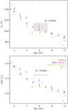 |
Fig. 10 Effective temperature (top) and bolometric luminosity (bottom) vs. age of HD 167665B (gray area) compared to evolutionary tracks from the COND (Baraffe et al. 2003), Saumon & Marley (2008) (for two treatments of the clouds), and Burrows et al. (1997) models assuming a 68.3% confidence interval of the dynamical mass of the companion (colored points with uncertainties). Small horizontal offsets are applied for clarity to all models except for COND. |
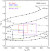 |
Fig. 11 Surface gravity as a function of the effective temperature predicted for several ages (black and solid curves) and companion masses (dashed curves) by the hybrid models of Saumon & Marley (2008). For comparison, the 1σ ranges derived for the effective temperature and surface gravity from atmospheric fits are shown (colored rectangles, Sect. 5.2). |
7.2 Formation mechanism
To evaluate a possible formation mechanism for HD 167665B, we compare its mass (or mass ratio to the star) and semi-major axis to model objects formed by the fragmentation of a collapsing cloud in Bate (2009) (Fig. 21) or by disk gravitational instability in Forgan & Rice (2013) and Vigan et al. (2017) (left panel of Fig. 8 in the latter paper). For the former process, most model objects with mass ratios similar to HD 167665B have semi-major axes in the range 20–5000 au. For the latter process, most model objects with masses similar to HD 167665b have semi-major axes in the range ~10–50 au. HD 167665B lies at a closer separation to the star compared to the bulk of the model predictions of both formation models, and we cannot exclude any of them. Similar conclusions are found for the benchmark brown dwarf HD 72946B (Maire et al. 2020a), which lies at a slightly larger semi-major axis, but is more massive (~6.5 au and 69.5 ± 0.5 MJ, respectively, Balmer et al. 2023).
Another diagnostic for the formation process would be the metallicity of the companion. For both disk gravitational instability and fragmentation of a collapsing cloud, it is expected to be close to the stellar metallicity. However, the metallicity of HD 167665B is poorly constrained in the atmospheric analysis (see fit with Sonora Bobcat models in Table 8).
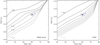 |
Fig. 12 Bolometric luminosity and mass of HD 167665B measured at 1σ (blue dot with dark gray area) and 3σ (light gray area) compared to isochrones of the hybrid models of Saumon & Marley (2008) (left, from top to bottom, 1, 2, 3, 4, 6, 8, and 10 Gyr) and of the COND model (right, from top to bottom, 1–10 Gyr in steps of 1 Gyr). |
7.3 Comparison with other benchmark brown dwarfs
HD 167665B is a new addition to a growing group of imaged brown dwarfs of spectral type T with dynamical mass measurements that will serve as valuable benchmarks for atmospheric and evolutionary models of cool substellar objects: GJ 758B (Thalmann et al. 2009; Brandt et al. 2019, 2021), HD4113C (Cheetham et al. 2018a), GJ 229B (Nakajima et al. 1995; Brandt et al. 2020, 2021), HD 13724B (Rickman et al. 2020; Brandt et al. 2021), HD 19467B (Crepp et al. 2014; Maire et al. 2020b; Brandt et al. 2021), e Indi Ba and Bb (McCaughrean et al. 2004; Chen et al. 2022), HIP 21152B (Bonavita et al. 2022; Kuzuhara et al. 2022; Franson et al. 2023), and possibly HD 47127B (Bowler et al. 2021) and HD 176535B (Li et al. 2023). With a semi-major axis of ~5.4 au, HD 167665B is the closest directly imaged BD companion to a star with a measured dynamical mass at the time of writing. This study is one of the first studies combining RV, astrometry, ground-based interferome-try, and high-contrast imaging, and shows the potential and complementarity of these tools, with Balmer et al. (2023).
Brandt et al. (2021) compare the measured mass, luminosity, and age of a sample of 12 brown dwarfs to evolutionary models, and find an overluminosity trend for younger or less massive companions and an underluminosity trend for older or more massive companions. Their reference evolutionary model is the hybrid cloudy model of Saumon & Marley (2008) for their whole sample. With a measured bolometric luminosity within 1σ from the predictions of the same evolutionary model and given our age constraints, HD 167665B appears to be consistent with evolutionary models. HD 19467B and HD 13724B, the closest analogs to HD 167665B according to our color-magnitude analysis (Fig. 4), are classified as underluminous and overlumi-nous, respectively. Nevertheless, the properties of HD 19467B would be consistent with the evolutionary models within 1.3σ. If we consider other known early to mid-T-type benchmark dwarfs older than 1 Gyr, ϵ Indi Ba and Bb appear to be consistent with the evolutionary models (Chen et al. 2022), whereas HD 176535B would be underluminous (Li et al. 2023).
8 Conclusions
We presented the direct imaging confirmation and the dynamical and spectral characterization of the brown dwarf companion to the field F9V star HD 167665 discovered using RV monitoring. The analysis of the stellar properties confirmed that the star is subsolar and suggests a mass of 1.054 ± 0.032 M⊙ and an age of 6.20 ± 1.13 Gyr. The companion was first imaged with GRAVITY using an on-sky position predicted from a joint fit of RV and proper motion anomaly data. Subsequent SPHERE imaging confirmed the detection and revealed a faint point source of contrast ΔH2 = 10.95 ± 0.33 mag at a projected angular separation of ~180 mas. We constrained the mass of HD 167665B to ~1.2%, 60.3 ± 0.7 MJ, based on a joint fit of the SPHERE and GRAVITY data with RV data from CORALIE and HIRES and astrometric data from HIPPARCOS and Gaia using the BINARYS tool, which provides a rigorous treatment of the HIPPARCOS IAD and the Gaia astrometric parameters.
The location of the brown dwarf in a color–magnitude diagram suggests a mid-T-type dwarf. A comparison of the SPHERE spectrum to template spectra suggests a spectral type of  . The fit of the SPHERE spectrophotometry and GRAVITY spectrum with synthetic spectra from the BT-Settl, ATMO SNEQ, Sonora Bobcat, and Morley+2012 libraries suggests an effective temperature of ~ 1000–1150 K and a surface gravity of ~5.0–5.4 dex. We also derive a bolometric luminosity
  dex.
dex.
The measured mass, luminosity, and age of the companion can only be reproduced within 3σ by the hybrid cloudy evolutionary models of Saumon & Marley (2008). Cloudless evolutionary models underpredict its luminosity given the age constraints. The formation of such a massive brown dwarf in a close-in orbit to a star appears atypical when comparing its mass and semi-major axis to synthetic populations predicted by disk gravitational instability and a stellar formation process. HD 167665B is a new addition to a growing sample of substellar companions with empirical mass measurements that will be valuable to benchmark theoretical mass–luminosity–age relations.
A measurement of the stellar radius using long baseline inter-ferometry may provide further clues to its evolutionary stage (see, e.g., Wood et al. 2019, for HD 19467, whose distance to the Sun is similar to that of HD 167665). Further imaging monitoring of the companion and the upcoming release of the Gaia epoch astrometry will further constrain its mass. Deeper spec-trophotometric measurements will be valuable to confirm or not its overluminosity with respect to the predictions of cloudless evolutionary models and better constrain its atmospheric properties. Finally, this study together with Balmer et al. (2023) exemplify the potential and complementarity of RV, astrometry, ground-based interferometry, and high-contrast imaging for the detailed characterization of substellar companions in the close-in environment of stars.
Acknowledgements
We thank an anonymous referee for a constructive report that helped to improve the manuscript. The authors thank the ESO Paranal Staff for support in conducting the observations and Eric Lagadec and Nadège Meunier (SPHERE Data Centre) for their help with the data reduction. This work has made use of recipes from the IDL libraries: IDL Astronomy Users’s Library (Landsman 1993) and Coyote (http://www.idlcoyote.com/index.html). It has also made use of the Python packages: NumPy (Oliphant 2006), emcee (Foreman-Mackey et al. 2013), corner (Foreman-Mackey 2016), Matplotlib (Hunter 2007), Astropy (Astropy Collaboration 2013, 2018), and dateutil (http://dateutil.readthedocs.io/). A.L.M. and S.L. acknowledge financial support from the Agence Nationale de la Recherche (ANR-21-CE31-0017). A.L.M. acknowledges support for the early stages of this publication from the European Research Council (ERC) under the European Union’s Horizon 2020 research and innovation program (Grant Agreement No. 819155). This work is supported by the French National Research Agency (ANR-15-IDEX-02), in particular through the funding of the “Origin of Life” project of the Univ. Grenoble Alpes. T.H. acknowledges support from the ERC under the Horizon 2020 Framework Program via the ERC Advanced Grant Origins 83 24 28. A.Z. acknowledges support from ANID – Millennium Science Initiative Program - Center Code NCN2021_080. This project received funding from the ERC under the European Union’s Horizon Europe research and innovation program (grant agreement No. 101053020, project Dust2Planets). J.S. receives funding from the Deutsche Forschungsgemeinschaft (DFG, German Research Foundation) under Germany’s Excellence Strategy – EXC-2094 – 390783311. We acknowledge financial support from the Programme National de Plané-tologie (PNP) and the Programme National de Physique Stellaire (PNPS) of CNRS-INSU in France. This work has also been supported by a grant from the French Labex OSUG@2020 (Investissements d’avenir - ANR10 LABX56). The project is supported by CNRS, by the Agence Nationale de la Recherche (ANR-14-CE33-0018). It has also been carried out within the frame of the National Centre for Competence in Research PlanetS supported by the Swiss National Science Foundation (SNSF). M.R.M. and S.D. are pleased to acknowledge this financial support of the SNSF. This work has made use of the SPHERE Data Centre, jointly operated by OSUG/IPAG (Grenoble), PYTHEAS/LAM/CeSAM (Marseille), OCA/Lagrange (Nice), Observatoire de Paris/LESIA (Paris), and Observatoire de Lyon, also supported by a grant from Labex OSUG@2020 (Investissements d’avenir – ANR10 LABX56). This publication has made use of VOSA, developed under the Spanish Virtual Observatory project supported by the Spanish MINECO through grant AyA2017-84089. VOSA has been partially updated by using funding from the European Union’s Horizon 2020 Research and Innovation Programme, under Grant Agreement n° 776403 (EXOPLANETS-A). This research has made use of the SIMBAD database and the VizieR Catalogue access tool, both operated at the CDS, Strasbourg, France. The original descriptions of the SIMBAD and VizieR services were published in Wenger et al. (2000) and Ochsenbein et al. (2000). This research has made use of NASA’s Astrophysics Data System Bibliographic Services. SPHERE is an instrument designed and built by a consortium consisting of IPAG (Grenoble, France), MPIA (Heidelberg, Germany), LAM (Marseille, France), LESIA (Paris, France), Laboratoire Lagrange (Nice, France), INAF – Osservatorio di Padova (Italy), Observatoire de Genève (Switzerland), ETH Zurich (Switzerland), NOVA (Netherlands), ONERA (France), and ASTRON (Netherlands), in collaboration with ESO. SPHERE was funded by ESO, with additional contributions from CNRS (France), MPIA (Germany), INAF (Italy), FINES (Switzerland), and NOVA (Netherlands). SPHERE also received funding from the European Commission Sixth and Seventh Framework Programs as part of the Optical Infrared Coordination Network for Astronomy (OPTICON) under grant number RII3-Ct-2004-001566 for FP6 (2004–2008), grant number 226604 for FP7 (2009–2012), and grant number 312430 for FP7 (2013–2016). This publication makes use of The Data & Analysis Center for Exoplanets (DACE), which is a facility based at the University of Geneva (CH) dedicated to extrasolar planets data visualisation, exchange and analysis. DACE is a platform of the Swiss National Centre of Competence in Research (NCCR) PlanetS, federating the Swiss expertise in Exoplanet research. The DACE platform is available at https://dace.unige.ch. This work has made use of data from the European Space Agency (ESA) mission Gaia (https://www.cosmos.esa.int/gaia), processed by the Gaia Data Processing and Analysis Consortium (DPAC, https://www.cosmos.esa.int/web/gaia/dpac/consortium). Funding for the DPAC has been provided by national institutions, in particular the institutions participating in the Gaia Multilateral Agreement.
Appendix A Comparison of extracted SPHERE spectrophotometry
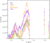 |
Fig. A.1 Comparison of the SPHERE spectrophotometry extracted with different data processing algorithms. The measurement uncertainties are shown at 1σ for all algorithms. |
We show in Fig. A.1 the comparison of the SPHERE spectrophotometry extracted with different data processing algorithms (see Sect. 3.1). The measurement uncertainties are given at 1σ. The comparison was performed in an earlier stage of the data analysis with a preliminary photometric calibration compared to the final analysis used in the main text. The null values correspond to spectral channels in which the companion is not detected. For the IFS spectrum, the ANDROMEDA and TRAP fluxes are systematically higher compared to the PCA, TLOCI, and PACO fluxes. The ANDROMEDA spectrum also shows a steeper slope compared to all other algorithms. We note a good agreement between the PCA, TLOCI, and PACO fluxes within the uncertainties around the peak in the J band. At shorter wavelengths, the detection of the companion is more challenging. While the PCA and TLOCI fluxes agree within the uncertainties around the peak in the Y band, the PACO fluxes are lower. For the IRDIS photometry in the H2 band, the extracted fluxes differ by 1.2 mag between the TRAP and PACO algorithms, whereas they agree within the uncertainties for the PCA, TLOCI, and ANDROMEDA algorithms. For the IRDIS photometry in the H3 band (which matches a methane absorption feature), the PCA, ANDROMEDA, and TRAP fluxes agrees within the uncertainties, whereas the PACO flux is lower. Therefore, we chose the PCA spectrophotometry for the spectral analysis. For consistency, we chose to use the PCA astrometry for the orbital analysis (the values agree within 2σ for all algorithms).
Appendix B Corner plot for the orbital fit
We show in Fig. B.1 the posterior distributions corresponding to the orbital fit described in Sect. 4.
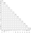 |
Fig. B.1 Corner plot of all the MCMC iterations for the orbital parameters, the mass of HD 167665 A and B, and the differences between the astrometric parameters with respect to the published IAD solution using the BINARYS tool (see text). The diagrams displayed on the diagonals represent the density of probability for the parameters. The off-diagonal diagrams show the correlations. |
Appendix C Color–magnitude diagram
To build the diagram in Fig. 4, we used spectra of M, L, and T dwarfs from the SpeX-Prism library (Burgasser 2014) and from Leggett et al. (2000) and Schneider et al. (2015) to generate synthetic photometry in the SPHERE filter passbands. The zero-points were computed using a flux-calibrated spectrum of Vega (Hayes 1985; Mountain et al. 1985). We also considered the spectra of young and/or dusty free-floating objects from Liu et al. (2013), Mace et al. (2013), Gizis et al. (2015), and of young companions (Wahhaj et al. 2011; Gauza et al. 2015; Stone et al. 2016; De Rosa et al. 2014; Lachapelle et al. 2015; Bailey et al. 2014; Rajan et al. 2017; Bonnefoy et al. 2014; Patience et al. 2010; Lafrenière et al. 2010; Chauvin et al. 2017; Delorme et al. 2017b; Cheetham et al. 2018a). The colors and absolute fluxes of the benchmark companions and isolated T-type objects were generated from the distance and spectra of these objects in Appendix B in Bonnefoy et al. (2018). To conclude, we used the spectra of Y dwarfs published in Schneider et al. (2015), Warren et al. (2007), Delorme et al. (2008), Burningham et al. (2008), Lucas et al. (2010), Kirkpatrick et al. (2012), and Mace et al. (2013) to extend the diagrams in the late-T and early-Y dwarf domain. We used the distances of the field dwarfs reported in Kirkpatrick et al. (2000), Faherty et al. (2012), Dupuy & Kraus (2013), Tinney et al. (2014), Beichman et al. (2014), and Luhman & Esplin (2016). We considered those reported in Kirkpatrick et al. (2011), Faherty et al. (2012), Zapatero Osorio et al. (2014), and Liu et al. (2016) for the dusty dwarfs. The companion distances were taken from van Leeuwen (2007) and Ducourant et al. (2014). We also added the T-type brown dwarf companions HD 4113C (Cheetham et al. 2018b), HD 13724B (Rickman et al. 2020), and HD 19467B (Maire et al. 2020b).
References
- Allard, F., Homeier, D., Freytag, B., & Sharp, C. M. 2012, EAS Pub. Ser., 57, 3 [NASA ADS] [CrossRef] [EDP Sciences] [Google Scholar]
- Astropy Collaboration (Robitaille, T. P., et al.) 2013, A&A, 558, A33 [NASA ADS] [CrossRef] [EDP Sciences] [Google Scholar]
- Astropy Collaboration (Price-Whelan, A. M., et al.) 2018, AJ, 156, 123 [Google Scholar]
- Bailey, V., Meshkat, T., Reiter, M., et al. 2014, ApJ, 780, L4 [Google Scholar]
- Balmer, W. O., Pueyo, L., Stolker, T., et al. 2023, ApJ, 956, 99 [NASA ADS] [CrossRef] [Google Scholar]
- Baraffe, I., Chabrier, G., Barman, T. S., Allard, F., & Hauschildt, P. H. 2003, A&A, 402, 701 [NASA ADS] [CrossRef] [EDP Sciences] [Google Scholar]
- Baraffe, I., Homeier, D., Allard, F., & Chabrier, G. 2015, A&A, 577, A42 [NASA ADS] [CrossRef] [EDP Sciences] [Google Scholar]
- Barbato, D., Ségransan, D., Udry, S., et al. 2023, A&A, 674, A114 [NASA ADS] [CrossRef] [EDP Sciences] [Google Scholar]
- Bate, M. R. 2009, MNRAS, 392, 590 [Google Scholar]
- Bayo, A., Rodrigo, C., Barrado Y Navascués, D., et al. 2008, A&A, 492, 277 [NASA ADS] [CrossRef] [EDP Sciences] [Google Scholar]
- Beichman, C., Gelino, C. R., Kirkpatrick, J. D., et al. 2014, ApJ, 783, 68 [NASA ADS] [CrossRef] [Google Scholar]
- Beuzit, J. L., Vigan, A., Mouillet, D., et al. 2019, A&A, 631, A155 [NASA ADS] [CrossRef] [EDP Sciences] [Google Scholar]
- Boccaletti, A., Sezestre, E., Lagrange, A.-M., et al. 2018, A&A, 614, A52 [NASA ADS] [CrossRef] [EDP Sciences] [Google Scholar]
- Boesgaard, A. M., Lum, M. G., Chontos, A., & Deliyannis, C. P. 2022, ApJ, 927, 118 [NASA ADS] [CrossRef] [Google Scholar]
- Bonavita, M., Fontanive, C., Gratton, R., et al. 2022, MNRAS, 513, 5588 [NASA ADS] [Google Scholar]
- Bonnefoy, M., Chauvin, G., Lagrange, A.-M., et al. 2014, A&A, 562, A127 [NASA ADS] [CrossRef] [EDP Sciences] [Google Scholar]
- Bonnefoy, M., Perraut, K., Lagrange, A. M., et al. 2018, A&A, 618, A63 [NASA ADS] [CrossRef] [EDP Sciences] [Google Scholar]
- Bowler, B. P., Endl, M., Cochran, W. D., et al. 2021, ApJ, 913, L26 [NASA ADS] [CrossRef] [Google Scholar]
- Brandt, G. M., Dupuy, T. J., Li, Y., et al. 2021, AJ, 162, 301 [NASA ADS] [CrossRef] [Google Scholar]
- Brandt, T. D. 2021, ApJS, 254, 42 [NASA ADS] [CrossRef] [Google Scholar]
- Brandt, T. D., Dupuy, T. J., & Bowler, B. P. 2019, AJ, 158, 140 [Google Scholar]
- Brandt, T. D., Dupuy, T. J., Bowler, B. P., et al. 2020, AJ, 160, 196 [Google Scholar]
- Bressan, A., Marigo, P., Girardi, L., et al. 2012, MNRAS, 427, 127 [NASA ADS] [CrossRef] [Google Scholar]
- Burgasser, A. J. 2014, ASI Conf. Ser., 11, 7 [Google Scholar]
- Burgasser, A. J., Geballe, T. R., Leggett, S. K., Kirkpatrick, J. D., & Golimowski, D. A. 2006, ApJ, 637, 1067 [Google Scholar]
- Burningham, B., Pinfield, D. J., Leggett, S. K., et al. 2008, MNRAS, 391, 320 [NASA ADS] [CrossRef] [Google Scholar]
- Burrows, A., Marley, M., Hubbard, W. B., et al. 1997, ApJ, 491, 856 [Google Scholar]
- Butler, R. P., Vogt, S. S., Laughlin, G., et al. 2017, AJ, 153, 208 [Google Scholar]
- Cantalloube, F., Mouillet, D., Mugnier, L. M., et al. 2015, A&A, 582, A89 [NASA ADS] [CrossRef] [EDP Sciences] [Google Scholar]
- Carbillet, M., Bendjoya, P., Abe, L., et al. 2011, Exp. Astron., 30, 39 [Google Scholar]
- Casagrande, L., Schönrich, R., Asplund, M., et al. 2011, A&A, 530, A138 [NASA ADS] [CrossRef] [EDP Sciences] [Google Scholar]
- Chabrier, G., Baraffe, I., Allard, F., & Hauschildt, P. 2000, ApJ, 542, 464 [Google Scholar]
- Chauvin, G., Desidera, S., Lagrange, A.-M., et al. 2017, A&A, 605, L9 [NASA ADS] [CrossRef] [EDP Sciences] [Google Scholar]
- Cheetham, A., Bonnefoy, M., Desidera, S., et al. 2018a, A&A, 615, A160 [NASA ADS] [CrossRef] [EDP Sciences] [Google Scholar]
- Cheetham, A., Ségransan, D., Peretti, S., et al. 2018b, A&A, 614, A16 [NASA ADS] [CrossRef] [EDP Sciences] [Google Scholar]
- Chen, M., Li, Y., Brandt, T. D., et al. 2022, AJ, 163, 288 [NASA ADS] [CrossRef] [Google Scholar]
- Claudi, R. U., Turatto, M., Gratton, R. G., et al. 2008, SPIE Conf. Ser., 7014, 70143E [Google Scholar]
- Crepp, J. R., Johnson, J. A., Howard, A. W., et al. 2014, ApJ, 781, 29 [Google Scholar]
- Cutri, R. M., Skrutskie, M. F., van Dyk, S., et al. 2003, VizieR Online Data Catalog: II/246 [Google Scholar]
- Cutri, R. M., Wright, E. L., Conrow, T., et al. 2013, VizieR Online Data Catalog: II/328 [Google Scholar]
- da Silva, L., Girardi, L., Pasquini, L., et al. 2006, A&A, 458, 609 [NASA ADS] [CrossRef] [EDP Sciences] [Google Scholar]
- De Rosa, R. J., Patience, J., Ward-Duong, K., et al. 2014, MNRAS, 445, 3694 [CrossRef] [Google Scholar]
- Delorme, P., Delfosse, X., Albert, L., et al. 2008, A&A, 482, 961 [NASA ADS] [CrossRef] [EDP Sciences] [Google Scholar]
- Delorme, P., Meunier, N., Albert, D., et al. 2017a, in SF2A-2017, ed. C. Reylé, P. Di Matteo, F. Herpin, E. Lagadec, A. Lançon, Z. Meliani, & F. Royer, 347 [Google Scholar]
- Delorme, P., Schmidt, T., Bonnefoy, M., et al. 2017b, A&A, 608, A79 [NASA ADS] [CrossRef] [EDP Sciences] [Google Scholar]
- Desidera, S., Chauvin, G., Bonavita, M., et al. 2021, A&A, 651, A70 [EDP Sciences] [Google Scholar]
- Dohlen, K., Langlois, M., Saisse, M., et al. 2008, SPIE Conf. Ser., 7014, 70143L [Google Scholar]
- Ducourant, C., Teixeira, R., Galli, P. A. B., et al. 2014, A&A, 563, A121 [NASA ADS] [CrossRef] [EDP Sciences] [Google Scholar]
- Dupuy, T. J., & Kraus, A. L. 2013, Science, 341, 1492 [NASA ADS] [CrossRef] [Google Scholar]
- El-Badry, K., Rix, H.-W., & Heintz, T. M. 2021, MNRAS, 506, 2269 [NASA ADS] [CrossRef] [Google Scholar]
- Faherty, J. K., Burgasser, A. J., Walter, F. M., et al. 2012, ApJ, 752, 56 [Google Scholar]
- Feng, F., Butler, R. P., Vogt, S. S., et al. 2022, ApJS, 262, 21 [NASA ADS] [CrossRef] [Google Scholar]
- Flasseur, O., Denis, L., Thiébaut, É., & Langlois, M. 2018, A&A, 618, A138 [NASA ADS] [CrossRef] [EDP Sciences] [Google Scholar]
- Foreman-Mackey, D. 2016, J. Open Source Softw., 1, 24 [Google Scholar]
- Foreman-Mackey, D., Hogg, D. W., Lang, D., & Goodman, J. 2013, PASP, 125, 306 [Google Scholar]
- Forgan, D., & Rice, K. 2013, MNRAS, 432, 3168 [Google Scholar]
- Franson, K., Bowler, B. P., Bonavita, M., et al. 2023, AJ, 165, 39 [NASA ADS] [CrossRef] [Google Scholar]
- Gaia Collaboration (Prusti, T., et al.) 2016, A&A, 595, A1 [NASA ADS] [CrossRef] [EDP Sciences] [Google Scholar]
- Gaia Collaboration (Brown, A. G. A., et al.) 2021, A&A, 649, A1 [NASA ADS] [CrossRef] [EDP Sciences] [Google Scholar]
- Gaia Collaboration (Arenou, F., et al.) 2023a, A&A, 674, A34 [CrossRef] [EDP Sciences] [Google Scholar]
- Gaia Collaboration (Vallenari, A., et al.) 2023b, A&A, 674, A1 [NASA ADS] [CrossRef] [EDP Sciences] [Google Scholar]
- Galicher, R., Boccaletti, A., Mesa, D., et al. 2018, A&A, 615, A92 [NASA ADS] [CrossRef] [EDP Sciences] [Google Scholar]
- Gauza, B., Béjar, V. J. S., Pérez-Garrido, A., et al. 2015, ApJ, 804, 96 [NASA ADS] [CrossRef] [Google Scholar]
- Gizis, J. E., Allers, K. N., Liu, M. C., et al. 2015, ApJ, 799, 203 [NASA ADS] [CrossRef] [Google Scholar]
- GRAVITY Collaboration (Abuter, R., et al.) 2017, A&A, 602, A94 [NASA ADS] [CrossRef] [EDP Sciences] [Google Scholar]
- Gray, R. O., Corbally, C. J., Garrison, R. F., et al. 2006, AJ, 132, 161 [Google Scholar]
- Guerri, G., Daban, J.-B., Robbe-Dubois, S., et al. 2011, Exp. Astron., 30, 59 [Google Scholar]
- Hayes, D. S. 1985, IAU Symp., 111, 225 [Google Scholar]
- Høg, E., Fabricius, C., Makarov, V. V., et al. 2000, A&A, 355, L27 [Google Scholar]
- Hunter, J. D. 2007, Comput. Sci. Eng., 9, 90 [NASA ADS] [CrossRef] [Google Scholar]
- Isaacson, H., & Fischer, D. 2010, ApJ, 725, 875 [Google Scholar]
- Jones, B. F., Fischer, D., & Soderblom, D. R. 1999, AJ, 117, 330 [NASA ADS] [CrossRef] [Google Scholar]
- Kervella, P., Arenou, F., Mignard, F., & Thévenin, F. 2019, A&A, 623, A72 [NASA ADS] [CrossRef] [EDP Sciences] [Google Scholar]
- Kervella, P., Arenou, F., & Thévenin, F. 2022, A&A, 657, A7 [NASA ADS] [CrossRef] [EDP Sciences] [Google Scholar]
- Kirkpatrick, J. D., Reid, I. N., Liebert, J., et al. 2000, AJ, 120, 447 [NASA ADS] [CrossRef] [Google Scholar]
- Kirkpatrick, J. D., Cushing, M. C., Gelino, C. R., et al. 2011, ApJS, 197, 19 [NASA ADS] [CrossRef] [Google Scholar]
- Kirkpatrick, J. D., Gelino, C. R., Cushing, M. C., et al. 2012, ApJ, 753, 156 [NASA ADS] [CrossRef] [Google Scholar]
- Kristensen, K., Nielsen, A., Berg, C. W., Skaug, H., & Bell, B. M. 2016, J. Stat. Softw., 70, 1 [CrossRef] [Google Scholar]
- Kuzuhara, M., Currie, T., Takarada, T., et al. 2022, ApJ, 934, L18 [NASA ADS] [CrossRef] [Google Scholar]
- Lachapelle, F.-R., Lafrenière, D., Gagné, J., et al. 2015, ApJ, 802, 61 [Google Scholar]
- Lacour, S., Wang, J. J., Nowak, M., et al. 2020, SPIE Conf. Ser., 11446, 114460O [NASA ADS] [Google Scholar]
- Lafrenière, D., Jayawardhana, R., & van Kerkwijk, M. H. 2010, ApJ, 719, 497 [CrossRef] [Google Scholar]
- Landsman, W. B. 1993, ASP Conf. Ser., 52, 246 [Google Scholar]
- Langlois, M., Vigan, A., Moutou, C., et al. 2013, in Proceedings of the Third AO4ELT Conference, eds. S. Esposito, & L. Fini, 63 [Google Scholar]
- Langlois, M., Gratton, R., Lagrange, A. M., et al. 2021, A&A, 651, A71 [NASA ADS] [CrossRef] [EDP Sciences] [Google Scholar]
- Leclerc, A., Babusiaux, C., Arenou, F., et al. 2023, A&A, 672, A82 [NASA ADS] [CrossRef] [EDP Sciences] [Google Scholar]
- Leggett, S. K., Allard, F., Dahn, C., et al. 2000, ApJ, 535, 965 [NASA ADS] [CrossRef] [Google Scholar]
- Li, Y., & Ezzeddine, R. 2023, AJ, 165, 145 [NASA ADS] [CrossRef] [Google Scholar]
- Li, Y., Brandt, T. D., Brandt, G. M., et al. 2023, MNRAS, 522, 5622 [NASA ADS] [CrossRef] [Google Scholar]
- Lindegren, L., Klioner, S. A., Hernández, J., et al. 2021, A&A, 649, A2 [EDP Sciences] [Google Scholar]
- Liu, M. C., Magnier, E. A., Deacon, N. R., et al. 2013, ApJ, 777, L20 [NASA ADS] [CrossRef] [Google Scholar]
- Liu, M. C., Dupuy, T. J., & Allers, K. N. 2016, ApJ, 833, 96 [NASA ADS] [CrossRef] [Google Scholar]
- Llorente de Andrés, F., Chavero, C., de la Reza, R., Roca-Fàbrega, S., & Cifuentes, C. 2021, A&A, 654, A137 [NASA ADS] [CrossRef] [EDP Sciences] [Google Scholar]
- Lucas, P. W., Tinney, C. G., Burningham, B., et al. 2010, MNRAS, 408, L56 [Google Scholar]
- Luck, R. E. 2017, AJ, 153, 21 [Google Scholar]
- Luhman, K. L., & Esplin, T. L. 2016, AJ, 152, 78 [NASA ADS] [CrossRef] [Google Scholar]
- Mace, G. N., Kirkpatrick, J. D., Cushing, M. C., et al. 2013, ApJS, 205, 6 [Google Scholar]
- Maire, A.-L., Langlois, M., Dohlen, K., et al. 2016, SPIE Conf. Ser., 9908, 990834 [Google Scholar]
- Maire, A. L., Baudino, J. L., Desidera, S., et al. 2020a, A&A, 633, L2 [NASA ADS] [CrossRef] [EDP Sciences] [Google Scholar]
- Maire, A. L., Molaverdikhani, K., Desidera, S., et al. 2020b, A&A, 639, A47 [NASA ADS] [CrossRef] [EDP Sciences] [Google Scholar]
- Marleau, G.-D., & Cumming, A. 2014, MNRAS, 437, 1378 [Google Scholar]
- Marleau, G.-D., Mordasini, C., & Kuiper, R. 2019, ApJ, 881, 144 [Google Scholar]
- Marley, M. S., Fortney, J. J., Hubickyj, O., Bodenheimer, P., & Lissauer, J. 2007, ApJ, 655, 541 [NASA ADS] [CrossRef] [Google Scholar]
- Marley, M. S., Saumon, D., Visscher, C., et al. 2021, ApJ, 920, 85 [NASA ADS] [CrossRef] [Google Scholar]
- Marois, C., Lafrenière, D., Doyon, R., Macintosh, B., & Nadeau, D. 2006, ApJ, 641, 556 [Google Scholar]
- Marois, C., Correia, C., Galicher, R., et al. 2014, SPIE Conf. Ser., 9148, 91480U [Google Scholar]
- Martinez, P., Dorrer, C., Aller Carpentier, E., et al. 2009, A&A, 495, 363 [NASA ADS] [CrossRef] [EDP Sciences] [Google Scholar]
- Masana, E., Jordi, C., & Ribas, I. 2006, A&A, 450, 735 [NASA ADS] [CrossRef] [EDP Sciences] [Google Scholar]
- Mawet, D., Milli, J., Wahhaj, Z., et al. 2014, ApJ, 792, 97 [Google Scholar]
- McCaughrean, M. J., Close, L. M., Scholz, R. D., et al. 2004, A&A, 413, 1029 [NASA ADS] [CrossRef] [EDP Sciences] [Google Scholar]
- Mermilliod, J. C. 2006, VizieR Online Data Catalog: II/168 [Google Scholar]
- Mesa, D., Gratton, R., Zurlo, A., et al. 2015, A&A, 576, A121 [NASA ADS] [CrossRef] [EDP Sciences] [Google Scholar]
- Monnahan, C. C., & Kristensen, K. 2018, PLoS ONE, 13, e0197954 [NASA ADS] [CrossRef] [Google Scholar]
- Mordasini, C., Marleau, G. D., & Mollière, P. 2017, A&A, 608, A72 [NASA ADS] [CrossRef] [EDP Sciences] [Google Scholar]
- Morley, C. V., Fortney, J. J., Marley, M. S., et al. 2012, ApJ, 756, 172 [NASA ADS] [CrossRef] [Google Scholar]
- Mortier, A., Santos, N. C., Sousa, S., et al. 2013, A&A, 551, A112 [NASA ADS] [CrossRef] [EDP Sciences] [Google Scholar]
- Mountain, C. M., Leggett, S. K., Selby, M. J., Blackwell, D. E., & Petford, A. D. 1985, A&A, 151, 399 [NASA ADS] [Google Scholar]
- Mugnier, L. M., Cornia, A., Sauvage, J.-F., et al. 2009, J. Opt. Soc. Am. A, 26, 1326 [NASA ADS] [CrossRef] [Google Scholar]
- Nakajima, T., Oppenheimer, B. R., Kulkarni, S. R., et al. 1995, Nature, 378, 463 [Google Scholar]
- Nowak, M., Lacour, S., Lagrange, A. M., et al. 2020, A&A, 642, L2 [NASA ADS] [CrossRef] [EDP Sciences] [Google Scholar]
- Ochsenbein, F., Bauer, P., & Marcout, J. 2000, A&AS, 143, 23 [NASA ADS] [CrossRef] [EDP Sciences] [Google Scholar]
- Oliphant, T. E. 2006, A Guide to NumPy (USA: Trelgol Publishing USA), 1 [Google Scholar]
- Pace, G., Castro, M., Meléndez, J., Théado, S., & do Nascimento, J. D.J. 2012, A&A, 541, A150 [NASA ADS] [CrossRef] [EDP Sciences] [Google Scholar]
- Patel, S. G., Vogt, S. S., Marcy, G. W., et al. 2007, ApJ, 665, 744 [Google Scholar]
- Patience, J., King, R. R., de Rosa, R. J., & Marois, C. 2010, A&A, 517, A76 [NASA ADS] [CrossRef] [EDP Sciences] [Google Scholar]
- Paunzen, E. 2015, A&A, 580, A23 [NASA ADS] [CrossRef] [EDP Sciences] [Google Scholar]
- Pavlov, A., Möller-Nilsson, O., Feldt, M., et al. 2008, SPIE Conf. Ser., 7019, 701939 [Google Scholar]
- Peretti, S., Ségransan, D., Lavie, B., et al. 2019, A&A, 631, A107 [NASA ADS] [CrossRef] [EDP Sciences] [Google Scholar]
- Perryman, M. A. C., Lindegren, L., Kovalevsky, J., et al. 1997, A&A, 323, L49 [Google Scholar]
- Phillips, M. W., Tremblin, P., Baraffe, I., et al. 2020, A&A, 637, A38 [NASA ADS] [CrossRef] [EDP Sciences] [Google Scholar]
- Queloz, D., Mayor, M., Naef, D., et al. 2000, in From Extrasolar Planets to Cosmology: The VLT Opening Symposium, eds. J. Bergeron, & A. Renzini Berlin: Springer, 548 [CrossRef] [Google Scholar]
- Rajan, A., Rameau, J., De Rosa, R. J., et al. 2017, AJ, 154, 10 [Google Scholar]
- Ramírez, I., Fish, J. R., Lambert, D. L., & Allende Prieto, C. 2012, ApJ, 756, 46 [CrossRef] [Google Scholar]
- Ramírez, I., Meléndez, J., Bean, J., et al. 2014, A&A, 572, A48 [Google Scholar]
- Reffert, S., & Quirrenbach, A. 2011, A&A, 527, A140 [NASA ADS] [CrossRef] [EDP Sciences] [Google Scholar]
- Rickman, E. L., Ségransan, D., Hagelberg, J., et al. 2020, A&A, 635, A203 [NASA ADS] [CrossRef] [EDP Sciences] [Google Scholar]
- Sahlmann, J., Ségransan, D., Queloz, D., et al. 2011, A&A, 525, A95 [NASA ADS] [CrossRef] [EDP Sciences] [Google Scholar]
- Samland, M., Bouwman, J., Hogg, D. W., et al. 2021, A&A, 646, A24 [NASA ADS] [CrossRef] [EDP Sciences] [Google Scholar]
- Saumon, D., & Marley, M. S. 2008, ApJ, 689, 1327 [Google Scholar]
- Schneider, A. C., Cushing, M. C., Kirkpatrick, J. D., et al. 2015, ApJ, 804, 92 [Google Scholar]
- Sneden, C. A. 1973, PhD thesis, The University of Texas at Austin, USA [Google Scholar]
- Soummer, R., Pueyo, L., & Larkin, J. 2012, ApJ, 755, L28 [Google Scholar]
- Stolker, T., Quanz, S. P., Todorov, K. O., et al. 2020, A&A, 635, A182 [EDP Sciences] [Google Scholar]
- Stone, J. M., Skemer, A. J., Kratter, K. M., et al. 2016, ApJ, 818, L12 [NASA ADS] [CrossRef] [Google Scholar]
- Tal-Or, L., Trifonov, T., Zucker, S., Mazeh, T., & Zechmeister, M. 2019, MNRAS, 484, L8 [Google Scholar]
- Thalmann, C., Carson, J., Janson, M., et al. 2009, ApJ, 707, 123 [Google Scholar]
- Tinney, C. G., Faherty, J. K., Kirkpatrick, J. D., et al. 2014, ApJ, 796, 39 [Google Scholar]
- Valenti, J. A., & Fischer, D. A. 2005, ApJS, 159, 141 [Google Scholar]
- van Leeuwen, F. 2007, A&A, 474, 653 [CrossRef] [EDP Sciences] [Google Scholar]
- Vigan, A., Moutou, C., Langlois, M., et al. 2010, MNRAS, 407, 71 [Google Scholar]
- Vigan, A., Bonnefoy, M., Ginski, C., et al. 2016, A&A, 587, A55 [NASA ADS] [CrossRef] [EDP Sciences] [Google Scholar]
- Vigan, A., Bonavita, M., Biller, B., et al. 2017, A&A, 603, A3 [NASA ADS] [CrossRef] [EDP Sciences] [Google Scholar]
- Vigan, A., Fontanive, C., Meyer, M., et al. 2021, A&A, 651, A72 [EDP Sciences] [Google Scholar]
- Vogt, S. S., Allen, S. L., Bigelow, B. C., et al. 1994, Proc. SPIE, 2198, 362 [Google Scholar]
- Wahhaj, Z., Liu, M. C., Biller, B. A., et al. 2011, ApJ, 729, 139 [NASA ADS] [CrossRef] [Google Scholar]
- Warren, S. J., Mortlock, D. J., Leggett, S. K., et al. 2007, MNRAS, 381, 1400 [CrossRef] [Google Scholar]
- Wenger, M., Ochsenbein, F., Egret, D., et al. 2000, A&AS, 143, 9 [NASA ADS] [CrossRef] [EDP Sciences] [Google Scholar]
- Wood, C. M., Boyajian, T., von Braun, K., et al. 2019, ApJ, 873, 83 [NASA ADS] [CrossRef] [Google Scholar]
- Wright, J. T., Marcy, G. W., Butler, R. P., & Vogt, S. S. 2004, ApJS, 152, 261 [Google Scholar]
- Xiao, G.-Y., Liu, Y.-J., Teng, H.-Y., et al. 2023, Res. Astron. Astrophys., 23, 055022 [CrossRef] [Google Scholar]
- Zapatero Osorio, M. R., Béjar, V. J. S., Miles-Páez, P. A., et al. 2014, A&A, 568, A6 [NASA ADS] [CrossRef] [EDP Sciences] [Google Scholar]
All Tables
Orbital parameters and dynamical mass of HD 167665B derived using the BINARYS tool.
Characteristics of the atmospheric model grids adjusted on the spectral energy distribution of HD 167665B (see text).
All Figures
|
Fig. 1 SPHERE contrast images of HD 167665 (see text). The white arrows indicate the position of HD 167665B. The central regions of the images are numerically masked out to hide bright stellar residuals. The white cross in each panel indicates the location of the primary star. The contrast scales are the same between the IRDIS images (top row) and between the IFS images (bottom row). The companion appears significantly fainter in the H3 image because the spectral filter matches methane absorption bands, hinting that the companion is a T-type sub-stellar object. The images were smoothed using a Gaussian filter with a 2 pixel width. |
| In the text | |
|
Fig. 2 GRAVITY χ2 maps of HD 167665 for epochs UT 2021 March 3 (left) and UT 2021 August 27 (right) centered on the pointed location on sky. The location of the companion is shown as a blue circle in each panel. The x- and y-axes are the offsets in RA and Dec with respect to the star. The field of view (dashed outer circles) corresponds to the fiber field of view (~60 mas). |
| In the text | |
|
Fig. 3 Sample of 1000 model orbits fitted on the HD 167665B data (red points) from RV (top left) and imaging (top right) using the BINARYS tool (see text). The sample was drawn from 10 000 MCMC solutions (Appendix B). The solution derived by the TMB algorithm is shown as green dots. The RV and HIPPARCOS IAD residus (left, from middle to bottom) and the imaging residus (right, from middle to bottom) are computed with respect to the TMB solution. |
| In the text | |
|
Fig. 4 Color-magnitude diagram of HD 167665B (red) using the IRDIS photometry. Template dwarfs (colored points) and a few young low-mass companions (black labels) are also shown for comparison. |
| In the text | |
|
Fig. 5 Atmospheric fitting of HD 167665B with BT-Settl models. Top: corner plot of the retrieved parameters: Teff, log ɡ, radius, parallax, SPHERE/IFS scaling factor, log(L/L⊙), and mass. Bottom: comparison of the best-fit model spectra (black and gray) and photometry (open blue squares) with the measured SED (filled data points). The black model spectrum corresponds to the best-fit solution, whereas the gray model spectra were randomly drawn from the posterior distributions. The fit residuals are shown in the bottom panel and the filter transmission curves of SPHERE/IRDIS in the top panel. |
| In the text | |
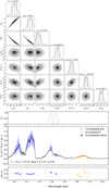 |
Fig. 6 Same as Fig. 5, but for ATMO SNEQ models. |
| In the text | |
|
Fig. 7 Same as Fig. 5, but for Sonora Bobcat models. The retrieved parameters in the corner plot are Teff, log ɡ, [M/H], radius, parallax, SPHERE/IFS scaling factor, log(L/L⊙), and mass. |
| In the text | |
|
Fig. 8 Same as Fig. 5, but for the Morley et al. (2012) models. The retrieved parameters in the corner plot are Teff, log ɡ, ƒsed, radius, parallax, SPHERE/IFS scaling factor, log(L/L⊙), and mass. |
| In the text | |
|
Fig. 9 SPHERE 5σ detection limits for contrast with respect to the star (top) and for mass (bottom) on putative additional companions around HD 167665 (see text). We also indicate the location of the companion for comparison (contrast in the H2 filter used in the contrast panel). |
| In the text | |
|
Fig. 10 Effective temperature (top) and bolometric luminosity (bottom) vs. age of HD 167665B (gray area) compared to evolutionary tracks from the COND (Baraffe et al. 2003), Saumon & Marley (2008) (for two treatments of the clouds), and Burrows et al. (1997) models assuming a 68.3% confidence interval of the dynamical mass of the companion (colored points with uncertainties). Small horizontal offsets are applied for clarity to all models except for COND. |
| In the text | |
|
Fig. 11 Surface gravity as a function of the effective temperature predicted for several ages (black and solid curves) and companion masses (dashed curves) by the hybrid models of Saumon & Marley (2008). For comparison, the 1σ ranges derived for the effective temperature and surface gravity from atmospheric fits are shown (colored rectangles, Sect. 5.2). |
| In the text | |
|
Fig. 12 Bolometric luminosity and mass of HD 167665B measured at 1σ (blue dot with dark gray area) and 3σ (light gray area) compared to isochrones of the hybrid models of Saumon & Marley (2008) (left, from top to bottom, 1, 2, 3, 4, 6, 8, and 10 Gyr) and of the COND model (right, from top to bottom, 1–10 Gyr in steps of 1 Gyr). |
| In the text | |
|
Fig. A.1 Comparison of the SPHERE spectrophotometry extracted with different data processing algorithms. The measurement uncertainties are shown at 1σ for all algorithms. |
| In the text | |
|
Fig. B.1 Corner plot of all the MCMC iterations for the orbital parameters, the mass of HD 167665 A and B, and the differences between the astrometric parameters with respect to the published IAD solution using the BINARYS tool (see text). The diagrams displayed on the diagonals represent the density of probability for the parameters. The off-diagonal diagrams show the correlations. |
| In the text | |
Current usage metrics show cumulative count of Article Views (full-text article views including HTML views, PDF and ePub downloads, according to the available data) and Abstracts Views on Vision4Press platform.
Data correspond to usage on the plateform after 2015. The current usage metrics is available 48-96 hours after online publication and is updated daily on week days.
Initial download of the metrics may take a while.