| Issue |
A&A
Volume 691, November 2024
|
|
|---|---|---|
| Article Number | A184 | |
| Number of page(s) | 13 | |
| Section | Planets and planetary systems | |
| DOI | https://doi.org/10.1051/0004-6361/202450900 | |
| Published online | 11 November 2024 | |
The outcome of collisions between gaseous clumps formed by disk instability
1
Department of Astrophysics, University of Zurich,
Winterthurerstrasse 190,
8057
Zurich,
Switzerland
2
Physics Institute, Space Research and Planetary Sciences, University of Bern,
Sidlerstrasse 5,
3012
Bern,
Switzerland
★★ Corresponding author; This email address is being protected from spambots. You need JavaScript enabled to view it.
, This email address is being protected from spambots. You need JavaScript enabled to view it.
Received:
28
May
2024
Accepted:
2
October
2024
Abstract
The disk instability model is a promising pathway for giant planet formation in various conditions. At the moment, population synthesis models are used to investigate the outcomes of this theory, where a key ingredient of the disk population evolution are collisions of self-gravitating clumps formed by the disk instabilities. In this study, we explored the wide range of dynamics between the colliding clumps by performing state-of-the-art smoothed particle hydrodynamics simulations with a hydrogen-helium mixture equation of state and investigated the parameter space of collisions between clumps of different ages, masses (1–10 Jupiter mass), various impact conditions (head-on to oblique collisions) and a range of relative velocities. We find that the perfect merger assumption used in population synthesis models is rarely satisfied and that the outcomes of most of the collisions lead to erosion, disruption or a hit-and-run. We also show that in some cases collisions can initiate the dynamical collapse of the clump. We conclude that population synthesis models should abandon the simplifying assumption of perfect merging. Relaxing this assumption will significantly affect the inferred population of planets resulting from the disk instability model.
Key words: equation of state / hydrodynamics / methods: numerical / planets and satellites: formation / planets and satellites: gaseous planets / protoplanetary disks
These authors contributed equally to this work.
© The Authors 2024
 Open Access article, published by EDP Sciences, under the terms of the Creative Commons Attribution License (https://creativecommons.org/licenses/by/4.0), which permits unrestricted use, distribution, and reproduction in any medium, provided the original work is properly cited.
This article is published in open access under the Subscribe to Open model. This email address is being protected from spambots. You need JavaScript enabled to view it. to support open access publication.
1 Introduction
The two leading models for the formation of gas giants are core accretion (Safronov 1972; Goldreich & Ward 1973; Pollack et al. 1996) and disk instability (DI) (Kuiper 1951; Boss 1997; Mayer et al. 2002). The former is considered to be the standard theory which suggests that giant planets form as a result of core formation followed by accretion of gas (mostly hydrogen and helium) from the proto-planetary disk.
While core accretion offers predictions that are consistent with many observations, it is challenged by the presence of massive giant planets around low-mass stars (Bakos et al. 2020; Delamer et al. 2024; Morales et al. 2019) and the formation of giant planets at wide orbital separations (Wagner et al. 2023; Currie et al. 2022; Sozzetti 2023). These observations prompt a further inquiry of the DI model, which offers possible cures for the short comings of core accretion (Helled et al. 2014).
The DI model suggests that when a massive protoplanetary disk experiences gravitational instabilities, it can fragment into self-gravitating clumps that contract further to become gas giant planets. For razor-thin axisymmetric disks, instabilities occur according to the Toomre criterion (Toomre 1964):
 (1)
(1)
where cS is the sound speed, κ the epicyclic frequency and Σ the surface density. In general, disks have a vertical extension and experience non-axisymmetric perturbations which explains why disk become unstable already at Q ≲ 1.7 (Durisen et al. 2007). The fragmentation of the disk occurs if it can cool rapidly, with the cooling time being comparable to the orbital period (O’Sullivan et al. 2005).
The resulting fragments are expected to have masses of a few times the Jovian mass MJ (Boley et al. 2010; Rogers & Wadsley 2012; Forgan & Rice 2011), although the exact mass distribution is unknown andis still being investigated (Deng etal. 2021; Kubli et al. 2023). During the first phase of the clump’s evolution, it contracts quasi-statically and hydrogen remains in molecular form. The clump is very extended with its radius being of the order of an astronomical unit (AU). The duration of this period, called the pre-collapse stage, is around 104−106 years (Decampli & Cameron 1979) depending on the clump mass (e.g. Helled & Schubert 2009; Helled & Bodenheimer 2010). As the clumps contract, their central temperature begins to rise and, when it reaches about 2000 K, the molecular hydrogen dissociates resulting in a dynamical collapse (e.g. Helled 2007; Helled & Schubert 2008). This second phase occurs on a dynamical timescale of a few years (Bodenheimer et al. 1980) resulting in a denser proto-planet with a radius of a few Jovian radii RJ which continues to contract and cool down. This is known as the post-collapse phase with an associated timescale of 109 years (Helled et al. 2014).
The DI model can be investigated using various computational methods. Ideally, one should simulate the entire proto-planetary disk in 3D using a hydrodynamics code which follows the clumps’ formation and evolution as well as the interactions of the clumps with the disk and each other. However, such simulations typically use a simplified prescription of the gas physics, such as, equation of state, opacities and cooling, and therefore are limited to simulating the earliest stages of a clump’s evolution (e.g. Mayer et al. 2007; Deng et al. 2021). In addition, the thermodynamics of the clumps is modelled in a simplified manner. Previous studies simulated the clump’s evolution using the appropriate equations of states and opacities; however, these models typically assume that the clump is isolated from the disk (e.g. Helled & Bodenheimer 2010; Vazan & Helled 2012) and therefore no interactions between clumps are considered.
In order to understand the planetary population in the DI model population synthesis models must be performed (Forgan et al. 2015; Humphries et al. 2019; Schib et al. 2023). Such models aim to simulate the formation and early evolution of each self-gravitating fragment and determine how interactions with the central star, the disk or other fragments affect its physical and orbital properties. A weakness of such models is that simplifying assumptions must be made when it comes to modelling the clumps’ structure and the relevant physics involved. For example, population synthesis cannot capture the complex dynamics of colliding bodies since the simulations drastically simplify the clump interactions by either neglecting them or by considering the clumps as point masses that perfectly merge when colliding.
Forgan et al. (2018) show that gravitational clump-clump interactions play a key role in sculpting the planetary population and motivated the investigation of collisions. Hall et al. (2017) performed hydrodynamics simulations of disk fragmentation and followed the formation and early evolution of clumps as well as their mutual interactions. Their results highlight the importance of gravitational interactions between clumps due to their effect on the clumps’ final orbits and internal structure. Indeed, clump-clump interactions can lead to a variety of outcomes such as mergers, fragmentation, tidal interactions or even total disruption.
In this paper we investigated the outcome of collisions between clumps using state-of-the-art 3D simulations. Our paper is organised as follows. Section 2 describes the initial conditions for the impacts, the equation of state used in the simulations and the collision outcomes classification. Our results are presented and discussed in Sect. 3. A summary and conclusions are presented in Sect. 4.
2 Methods
The simulations were performed using the smoothed particle hydrodynamics (SPH) method (Monaghan 1992). SPH is well suited to model collisions and was applied to different impact regimes, ranging from Asteroids (Raducan & Jutzi 2022; Jutzi et al. 2022), terrestrial (Kegerreis et al. 2020; Timpe et al. 2023; Chau et al. 2018) to giant planets (Reinhardt et al. 2020; Kegerreis et al. 2018; Woo et al. 2022). It exhibits great conservation properties, can handle geometries with high levels of deformation and tracks the fate of the material due to its Lagrangian nature. Our work constitutes the first application of SPH to the collision regime of proto-planetary clumps. For this study, we used a novel HPC implementation (Meier et al., in prep) of SPH within the gravity code pkdgrav3 (Potter et al. 2017). This SPH code leverages pkdgrav3, particularly its speed of gravity calculation on GPU/CPU parallel computers, while being a general SPH implementation with improvements for planetary collision simulations (Reinhardt & Stadel 2017; Reinhardt et al. 2020; Meier et al. 2021; Ruiz-Bonilla et al. 2022).
2.1 Initial conditions for the collisions
The initial conditions for the collision simulations comprise of the pre-impact models of the two clumps (initial density, temperature, pressure profiles), the initial separation, the relative velocity at which they collide and the impact angle.
The pre-impact models of the clumps were taken from Helled & Bodenheimer (2010) who modelled the pre-collapse evolution of clumps using 1D hydrodynamic simulations. They considered different clump masses ranging from 1 to 10 MJ. These models provide radial density, temperature and internal energy profiles of each clump. We considered four different clump masses of 1, 3, 5 and 10 MJ. For each mass we then considered three different models that correspond to different evolutionary stages: the very extended stage, meaning early evolution (henceforth called ‘young’), right before dynamical collapse (‘evolved’) and at the median time between those two stages (‘mid’).
To obtain a low-noise particle representation of the models, we used the ballic code (Reinhardt & Stadel 2017). The particle representation was then evolved in isolation with pkdgrav3 until it reached equilibrium. Especially for young clumps the relaxation process requires adding a damper term due to their large extension and low density making them more sensitive to noise.
The number of particles used to represent each clump was chosen so that all particles in the simulation had the same mass to ensure numerical stability. We resolved the lowest mass, that is the 1 MJ clump, with 105 particles meaning that all the other clumps had a higher resolution of 3 × 10⁵, 5 × 10⁵ and 106 for clumps with masses of 3, 5 and 10 MJ, respectively. Using this resolution allows for the investigation of a large parameter space with a high reliability with reasonable computational resources.
The initial conditions were set up such that the collision occurs in the xy-plane with the clump velocities being parallel to the x-axis at impact. In order to account for tidal deformation before the collision the clumps started with an initial separation of 5Rcrit, where Rcrit = R1 + R2 is the sum of the radii of both clumps (see Figure A.1 in the Appendix A for details).
The relative velocities at impact υimp that we investigated are normalised to the mutual escape velocity, defined as:
 (2)
(2)
with M1, M2 and R1, R2 being the masses and radii of the colliding clumps. For the majority of our simulations, we considered the interval 1 < υimp/υesc ≤ 2. This corresponds to impact velocities of a few km s−1 which is comparable to the orbital velocity at 100 AU assuming a solar mass star. Note that the possible range of relative velocities between two clumps orbiting a central star depends on the distance from the star and the eccentricity and inclination of the clump’s orbits. Collisions between clumps are expected to be above the mutual escape velocity even at large radial separations. We used the impact parameter b when the two clumps were in contact to parameterise the alignment of the collision. It is related to the impact angle by b = sin θ. A head-on collision corresponds to b = 0 and a grazing collision to b = 1 , where the clumps only interact through tidal forces. In this study, we investigated collisions with 0 ≤ b ≤ 0.7.
2.2 Equation of state
The adopted equation state (EoS) determines the type of material that is simulated. In this study, we used a realistic EoS modelling a mixture of the two most abundant gases in the proto-planetary disk, Hydrogen (H) and Helium (He). Initially developed by Saumon et al. (1995) for low-mass stars, brown dwarfs and giant planets, the SCvH (Saumon, Chabrier, van Horn) EoS models pure H, pure He and H-He mixtures with their non-ideal effects including ionisation, dissociation and formation of molecules. We will show in Sect. 3 that these features are crucial for modelling the dynamics of clump collisions. The EoS was extended to lower pressures and temperatures as described in Vazan et al. (2013) to cover the conditions for the study of clumps since they tend to be very diffuse and cold. The H-He mixture with a proto-solar composition of exactly 72.2% H and 27.8% He (Asplund et al. 2009) was calculated using the additive-volume rule.
Collision outcomes.
2.3 Collision outcomes
In order to find gravitationally bound clumps after the collisions and to distinguish them from the surrounding ejecta, we used the group finder skid (N-Body Shop 2011) with parameters nSmooth = 3200 and tau = 0.06. The simulations were run until the number of clumps and the bound mass had converged.
We then quantified the outcomes through the ratio of final total bound mass to initial total mass Mtot combined with the number of remaining fragments Nfra𝑔 after the collision. The classification of the collision outcomes is summarised in Table 1. In some cases, the fragments can survive a first collision but remain gravitationally bound and re-collide later to merge. These so called graze-and-merge collisions form a sub-regime of mergers and are at the transition to the hit-and-run regime (Stewart & Leinhardt 2012; Chau et al. 2021) but can require more simulation time to be resolved (Timpe et al. 2023).
3 Results and discussion
In total, we performed over two hundred simulations whose results are organised here according to the classification presented below and in Table 1. A summary of all the simulations with their initial conditions is listed in Table A.1. Table A.2 lists the occurrence of each type of outcome depending on the pair of colliding clumps. The collision outcomes depend on the clump mass and age as well as the impact parameter and velocity. The parameter space we considered here captures the transition between a large diversity of post-collision states.
3.1 Mergers
We defined a merger as a collision between two clumps resulting in a single gravitationally bound object. In a perfect merger (PM), as assumed in population synthesis models, this object contains the sum of their masses. However, in our set of simulations PM are very rare even for the most favourable conditions, that is for evolved (and therefore more compact) clumps and oblique impacts at υimp ~ υesc. Of all the 40 impact simulations between evolved clumps of different masses we find that only four result in PM, two of them being graze-and-merge collisions (for details see Sect. 2.3).
Figure 1 shows the distribution of the post-impact bound mass for mergers and combined mass of the two fragments for hit-and-run collisions (HRC), in both cases the mass is normalised to the initial total mass in the collision. The majority of observed mergers are erosive with more than 5% of mass loss after the collision and therefore are not classified as PM.
Figure 2 shows an example of an erosive merger between two evolved 5 MJ clumps colliding with b = 0.3 and υimp/υesc = 1.5. The snapshots are slices in the ɀ-direction and show how the clumps collide, merge, and finally reach a hydro-static equilibrium. An important aspect of those collisions is their large scale compared to planetary collisions. This example shows how the clumps collide and spread out material on distances in the order of the AU. For such extended objects the point-mass approximation used in population synthesis models is inappropriate.
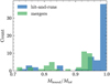 |
Fig. 1 Distribution of final bound mass fraction for post-collision states in the case of a merger (see Sect. 3.1) or a hit-and-run (see Sect. 3.2). The majority of mergers are erosive while there are mainly perfect rather than erosive hit-and-runs. Statistics for disruptions are shown in Fig. 3. |
3.2 Hit-and-run collisions
For impact velocities above the mutual escape velocity, oblique collisions result in hit-and-run collisions (HRC) where both clumps survive the encounter with a deviated trajectory after exchanging mass and angular momentum. Figure 3 shows the distribution of all the observed HRC depending on b and υimp/υesc. The majority of such events are preserving the mass of the clumps as shown in Fig. 1. Erosive HRC, where part of the bodies mass is lost due to the impact, are less common.
This is a result of the large radial density gradients inside the clumps. Most of their mass is contained within their inner layers, and therefore erosion of the outer layers by grazing collisions is less significant. The magnitude of the erosion strongly depends on the clump’s age since young clumps have lower central densities compared to evolved clumps, making them prone to lose more material during an HRC.
We observe that a change of the impact parameter affects the core’s density: the more oblique the collision, the higher the inner density of the remnants. A larger impact parameter results in remnants resembling the pre-collision clump profiles with only the outer layers being perturbed. More head-on collisions allow a greater exchange of kinetic energy and angular momentum. This leads to the spreading of material outwards due to the induced rotation and shock heating. This also affects the inner structure of the clump and can reduce the core density by almost an order of magnitude. Figure 4 illustrates this phenomenon by showing the radial density profiles for remnants of collisions between two mid 10 MJ clumps at υimp/υesc = 1.5 with the exact same initial conditions except a varying impact parameter. The post-collision angular momentum of the clumps is twice as large for b = 0.5 than for b = 0.7, which corresponds to 2% and 0.7% of the respective initial orbital angular momentum of the system.
While HRC are very common during the formation of rocky planets (e.g. Asphaug et al. 2006; Kokubo & Genda 2010), it remains unclear whether such events are common for gaseous clumps. In case they occur as frequently as for rocky planets, HRC need to be considered in population synthesis models since they deviate the trajectory of the clumps and reduce their kinetic energy. For clumps, HRC preserve the bound mass better than mergers but can still affect the stability of the clump in future encounters since a higher core density allows the clump to be sufficiently gravitationally bound to survive further collisions.
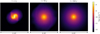 |
Fig. 2 Snapshots of slices in the ɀ-direction from the simulation of an erosive merger between two evolved 5 MJ clumps colliding with b = 0.3 and υίmp/υesc = 1.5. Since the collision is oblique, spiral structures are emerging but are then falling back onto the bound remnant until it reaches a spherically symmetric equilibrium state containing 72% of the initial total mass. |
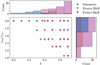 |
Fig. 3 Distribution of all observed erosive/perfect hit-and-runs (see Sect. 3.2) and disruptive collisions (see Sect. 3.3) depending on impact parameter and impact velocity. Hit-and-runs are favoured by oblique collisions and at the transition to the other regimes, they become erosive. Disruptions are favoured by high impact velocities and head-on collisions. |
3.3 Disruption
Collisions with high impact velocities and low impact angles can lead to significant mass loss or even destruction of the clumps. If more than half of the initial total mass is lost, we refer to the outcome of the collision as ‘disruption’. Such disruptions occur when the shock wave accelerates a significant amount of bound material beyond the escape velocity, ejecting it out of the clump’s gravitational potential. Clumps tend to be weakly bound, especially when they are young and are not very massive, that is the 1 and 3 MJ clumps in our simulations. As a result, their escape velocity is low and disruptive collisions are much more common than for compact and dense objects like rocky planets. In our set of collisions, we observe that these outcomes are favoured by large impact velocities and frontal collisions as shown in Fig. 3.
Figure 5 shows an example of a collision between a mid 10 MJ and a mid 5 MJ clumps with b = 0 and υimp/υesc = 2 that leads to a super-critical disruption. The strong shock wave caused by the collision propagates in a symmetric way since the collision is head-on. The material is ejected and no bound mass is left after the collision.
Disruption is more common with younger clumps since they are more extended and are less gravitationally bound: while the transition to disruption for evolved clumps is at υimp/υesc 2 (corresponding to velocities in the order of 7–9 km s−1), young clumps can already be disrupted by collisions at υimp/υesc 1.5 (in the order of 2–3 km s−1). Such velocities are comparable to the Keplerian velocity at 80 AU around a solar mass star. Therefore, disruptive outcomes could be very common during the early evolution of clumps and should be considered in population synthesis models.
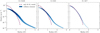 |
Fig. 4 Radial profiles for the density of hit-and-run remnants from υimp/υesc = 1.5 collisions between two mid 10 MJ clumps (the two remnants have the same profile due to symmetry). Only the gas with a density higher than 10−12 g cm−3 is displayed. The profile of the mid 10 MJ model is shown for reference. For each impact parameter the post-collision bound mass to total mass ratio is respectively 95.3%, 97.5% and 99.7% with the angular momentum of the remnant being 2.7%, 2% and 0.7% of the initial angular momentum of the collision, respectively. Head-on collisions essentially perturb the structure of the colliding clumps more than oblique collisions. |
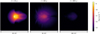 |
Fig. 5 Snapshots of slices in the ɀ-direction from the simulation of a super-critical disruption between mid 10 and 5 MJ clumps with b = 0 and υimp/υesc = 2. The shock wave propagates in both clumps and accelerates the gas beyond the mutual escape velocity. The ejected material is very low in density and is distributed over ~100 AU (note the different length scale of each frame). This event clearly shows how the population of clumps can decrease as a result of a collision. |
3.4 Core collapse
Some of the simulations, consisting of mid and evolved clumps involved in frontal collisions exhibit a fast and intense increase of density in distinct regions where they reach 1 g cm−3 compared to the maximal value of about 10−6 g cm−3 reached by the regular collisions. The time span needed to reach those high densities is in the order of a few years, which is much shorter than the entire collision timescale1.
Figure 6 shows such an event between evolved 10 and 5 MJ clumps in a collision with b = 0 and υimp/υesc = 1.05. We see the formation of a collapsing region behind the shock front that leads to a denser and more compact core. In this example, the bound mass of the remnant is 12.04 MJ which corresponds to ~77% of the initial total mass.
By compressing the gas during the collision, its pressure, density and temperature increase. The entropy also increases due to shock heating but in the case of adiabatic decompression such as during shock release, the evolution is isentropic. While the isentropes in the low pressure and temperature range of the SCvH table are identical to those of an ideal gas with a suitable molecular mass, there is a change at around log T ≃ 3. From that point, all isentropic curves exhibit a relatively flat region in the sense that the density increases by several orders of magnitude without a significant increase in temperature.
This kink in the isentropes corresponds to a phase transition since at these temperatures the molecular hydrogen starts to dissociate (Saumon et al. 1995). The kinetic energy gained from the collision is converted into energy for breaking the molecular bonds of the gas. Since the thermal pressure cannot balance gravity at these augmented densities, the clump is no longer in hydrostatic equilibrium leading to a collapse that occurs on a timescale of the order of the free-fall time  (e.g. Bodenheimer et al. 1980; Helled & Schubert 2009; Helled & Bodenheimer 2010). By calculating tff with the mean density of the clumps we indeed find that it is ~2 years, which is consistent with our simulations that were run through the collapse phase.
To investigate the collapse stage, the SPH particles of the same simulation snapshots from Fig. 6 are shown in the ρ − T diagram with curves of constant entropy in Fig. 7. The first frame shows how, during the collision, the particles are compressed and entropy increases due to shock heating. Once particles enter the flat region corresponding to molecular hydrogen dissociation, the dynamical collapse is initiated. After the collision, most of them reach the upper-right region of the diagram and stay with these high densities and temperatures: these are the ones making up the core. The innermost part of the core stays on its isentrope while the rest of the clump has been shock heated during the rapid in fall.
The simulations show that the collapsing region is behind the shock wave due to the lower thermal pressure that acts against gravity. Indeed, within the shock front the evolution is non-adiabatic (see Sect. 2) and gas heating provides support against collapse. Nevertheless, the collapsed region manages to pierce through the shock front after having formed and then accretes more mass due to its high density.
After the collapse, the remnant evolves towards hydrostatic equilibrium and regains spherical symmetry. Figure 8 compares the radial density and temperature profiles of the remnant to the initial models of the two colliding clumps. The differences in temperature and density are significant. The central part with a radius of a few RJ, is almost at ρ = 1 g cm−3 which corresponds to Jupiter’s mean density and the temperatures at around 70 000 K, comparable to central temperatures expected from the core accretion model (Müller et al. 2020). In principle, some energy should be lost via radiative cooling which is not considered in the simulations. As a result, our inferred temperature should be taken as upper bounds.
In order to investigate the physical nature of this outcome, the exact same collisions were simulated using an ideal gas EoS. These simulations do not result in dynamical collapse but are classified either as erosive mergers or, for high impact velocities, as disruptions, as defined in Table 1. This highlights the importance of using appropriate EoSs in impact simulations. As another sanity check, we performed a resolution study on a core collapse event between two evolved 10 MJ colliding with b = 0 and υimp/υesc = 1.05 to check whether this phenomenon is resolution dependent. The simulations with N = 105, 106 and 107 particles all experience the same dynamical collapse around the same time step which further supports that it is not a numerical artefact but indeed a physical event being captured by the SPH code.
More than 25% of the simulations lead to a dynamical collapse and it is more common for simulations with evolved clumps. That is because younger clumps require more energy to reach molecular hydrogen dissociation but are also more easily disrupted by strong shocks. On the other hand, evolved clumps are denser and hotter to begin with and therefore a collision can trigger the molecular dissociation for a wider range of impact parameters and velocities. Evolved clumps are also more stable against disruption due to their compactness and therefore the kinetic energy of the collision can efficiently contribute to the collapse without destroying the clump. Earlier collapse can also be initiated for collisions between clumps that are in the middle of the pre-collapse evolution (see Sect. 3.5). Even collisions of mixed ages can trigger the dynamical collapse within the clumps, as we observe for instance in those between young 3 MJ and evolved 10 MJ clumps, where the collision is triggered within the 10 MJ clump.
The initiation of a dynamical collapse via collisions shortens the pre-collapse stage of clumps. This would affect the inferred population since the remnants resulting from the dynamical collapse have higher chances to survive. As a result, this mechanism should be considered by population synthesis models.
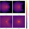 |
Fig. 6 Snapshots of slices in the ɀ-direction from the simulation of a collapsing collision between evolved 10 and 5 MJ clumps with b = 0 and υimp/υesc = 1.05. During the impact a compact region is forming behind the shock front in which the density increases by several orders of magnitude (top panels). At a later stage the collapsed region pierces through the shock front (bottom left panel) and regains hydrostatic equilibrium (bottom right panel). After the collision 77 % of the total colliding mass remains bound. Such collisions are a pathway to shorten the pre-collapse stage and influence the survival of the clumps in the proto-planetary disk. |
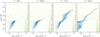 |
Fig. 7 Evolution of the SPH particles from Fig. 6 in the logarithmic ρ − T plane, in which the curves are (ρ, T) at constant entropy and the flat regions are phase transitions, namely dissociation of molecular hydrogen. Dotted red lines indicate where the original EoS table was extrapolated and the thermodynamic quantities can exhibit unphysical behaviour. The structures of the two colliding clumps can be distinguished from each other in the first frames but are then mixed by the impact. |
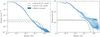 |
Fig. 8 Radial density and temperature profiles for the SPH particles of the remnant resulting from the collapsing collision displayed in Fig. 6. Only the particles with a density higher than 10−11 g cm−3 are shown. The bound mass of the remnant is 12.04 MJ amounting to 77% of the initial total mass. The densities and temperatures of the collision remnant are extremely high compared to the initial evolved 10 and 5 MJ clump models, whose profiles are shown for reference. A kink in the temperature at R = 10−3 AU is due to shock heating of material falling onto the central dense core. |
3.5 Overview
In this section, we summarise the outcomes of the different collision simulations. For different combinations of clump mass and age we plotted the outcomes defined in Table 1, as well as the core collapse, on a diagram with b and υimp as coordinates allowing for an overview of the results.
Figure 9 shows such a diagram for impacts between two evolved 10 MJ clumps. The diagram for two colliding evolved 5 MJ clumps looks exactly the same suggesting that the age and mass ratio is more relevant than the total colliding mass. Evolved and massive clumps have higher chances to collapse as a result of a collision since they are hotter, denser and more resistant against disruption compared to young and low-mass clumps. If the impact velocity is too high, there is a risk of eroding or disrupting both clumps when the collision occurs at low impact parameters. For more oblique impacts both clumps survive hit-and-run collisions. Erosive or perfect mergers are observed only in a limited region of this parameter space. This means that if two evolved clumps collide, they are more likely to retain their initial masses and have higher chances to evolve into giant planets as they can reach the dynamical collapse stage faster. It is still unclear whether such collisions are more common for impacts below the escape velocity since they might also collapse (see discussion below).
Figure 10 shows the same diagram for collisions between mid 10 MJ and mid 5 MJ clumps. While the mass ratio is different from 1:1, the overall structure is similar to the outcomes of collisions between two evolved 10 MJ clumps. Since the mid clumps are younger, they are more extended and therefore more vulnerable for disruption. As a result, PM does not occur and the mergers that do take place are erosive. Head-on collisions lead to disruption more often and the region where collapse can be initiated is smaller compared to evolved clumps. If a collision can initiate dynamical collapse, the duration of the pre-collapse stage of mid clumps is halved. In the case of a 5 MJ clump, this corresponds to 1.2 × 10⁴ instead of 2.4 × 10⁴ years. This significantly improves the likelihood of surviving future encounters.
Figure 11 shows the outcomes of two colliding young 3 MJ clumps. In this case collisions do not initial dynamical collapse. Young and less massive clumps are very fragile and easy to disrupt; however, they can still survive after HRC. We find no PM in this range of parameters. In fact, for a purely head-on collision PM occurs only for an impact velocity as low as υimp = 0.7 υesc which corresponds to a relative velocity of ~1.2 km s−1. We therefore conclude that when young clumps collide the assumption of PM is inappropriate.
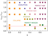 |
Fig. 9 Collision outcomes from simulations of two evolved 10 MJ clumps. The markers represent the real data acquired from the simulations. The data point at (b, υimp) = (0.65, 1.05) is a case of graze-and-merge impact where ≥95% of the mass remains gravitationally bound. This plot includes additional simulations at impact velocities below the mutual escape velocity (dashed red line). Head-on collisions with υimp/υesc < 1 still trigger dynamical collapse while more oblique impacts result in erosion or hit-and-run. |
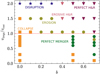 |
Fig. 10 Collision outcomes from simulations of two mid 10 and 5 MJ clumps. There are no PM in this range of parameters and the collapse region becomes smaller compared to Fig. 9. Additional simulations at impact velocities below the mutual escape velocity (dashed red line) show that head-on collisions with ~350 m s−1 initiate dynamic collapse. Only very grazing impacts can result in simple PM (see discussion in Section 3.6). |
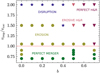 |
Fig. 11 Collision outcomes from simulations of two young 3 MJ clumps. Such clumps are very extended and have low densities. Therefore, their gravitational binding energy is very low and impacts result in either erosion or disruption. PM or dynamic collapse are not observed. Additional simulations at impact velocities below the mutual escape velocity (dashed red line) show that head-on or very grazing (b ~ 0.7) impacts with υimp/υesc ≥ 0.8–0.9 corresponding to 1.36 km s−1 to 1.54 km s−1 still lead to erosion. Only intermediate impact parameters result in PM (see discussion in Section 3.6). |
3.6 Low velocity impacts
All the simulations presented above have impact velocities above the mutual escape velocity. Although low velocity collisions are expected to be less common, in this section we performed additional simulations of head-on (b = 0) and oblique (b = 0.5, 0.7) impacts forthe clump models shown in Figs. 9–11 with velocities lower than the mutual escape velocity.
The results of such collisions between two evolved 10 MJ clumps are shown in Fig. 9. We find that head-on collisions can still trigger dynamical collapse and that grazing impacts lead to erosion or erosive hit-and-run collisions. Even for impacts below the mutual escape velocity we find that perfect mergers are a relatively rare outcome which occurs only for very grazing and low velocity collisions. The outcomes of collisions between two mid 10 MJ and 5 MJ clumps are shown in Fig. 10. Such collisions can lead to a dynamical collapse even for very low impact velocities. Grazing impacts above the mutual escape velocity result in erosion of hit-and-run, and collisions with υimp/υesc ≥ 0.6 for b = 0.5 and υimp/υesc ≥ 0.3 for b = 0.7 can lead to perfect mergers. Finally, we find that collisions between two young 3 MJ clumps (Fig. 11) are still erosive slightly below the mutual escape velocity if they are head-on (b = 0) or very grazing (b = 0.7). For the other cases collisions can lead to PM. Overall, we conclude that even for collisions with υimp/υesc < 1 the assumption of PM is often inappropriate. It is yet to be determined how relevant low velocity and oblique collisions are for young clumps. Preliminary results from population synthesis models in the disk instability scenario (Schib et. al., in prep.) suggest that impacts below the mutual escape velocity are very rare and that head-on collisions are more common.
3.7 Limitations and future work
While this study constitutes a first step in understanding the dynamics of colliding proto-planetary clumps, future studies should continue the investigation of this topic including more processes and a larger parameter space as we discuss below.
First, future research could obtain the impact conditions from disk simulations which follow the formation and evolution of clumps formed by DI. This could provide a more realistic parameter space for studying collisions in terms of clump sizes and masses, ages, as well as impact parameters and impact velocities, location of collision within the disk, etc. In turn, implementing a more realistic treatment of collisions in population synthesis models, for example, by using scaling laws inferred from SPH simulations, will affect the impact conditions obtained from such models highlighting the interplay between SPH and disk simulations.
Second, this work did not include pre-impact rotation. Investigating and quantifying the effect of pre-impact rotation is important since this effect could provide an additional stabilisation against gravitational contraction and affect the outcome of collisions. Since the impact simulations cover a time scale of hundreds of years, the heliocentric orbits of the clumps and their cooling as well as the effect of the disk on the clumps should also be considered. Similarly, the presence of magnetic fields could also affect the disk’s evolution and the final properties of the clumps (Deng et al. 2021; Kubli et al. 2023).
Third, our collision simulations do not account for the tidal interaction with the central star. As a result, clump masses inferred in our simulations correspond to an upper limit. The exact final mass of the merger remnants could be estimated using the Hill radius (Hamilton & Burns 1992) and would depend on the stellar mass and semi-major axis. Future studies could include the influence of the central star by directly adding its gravitational field during the collisions.
Fourth, it would be desirable to further investigate the shock-induced dynamical collapse and assess its significance in the DI model for giant planet formation. This could lead to a possible stimulated formation pathway along the same lines of shock-induced star formation due to collisions of molecular clouds or galaxies (Scoville et al. 1986; Jog & Solomon 1992).
Finally, future research could focus on fly-by events with the closest separation being larger than Rcrit to further investigate pure tidal interactions between the clumps and to determine whether continuous fly-bys have the ability to critically shape the body, a possible mechanism inspired by galactic dynamics (Moore et al. 1996).
4 Summary and conclusions
We investigated the outcome of collisions between planetary clumps formed by DI using the SPH code pkdgrav3 and the SCvH EoS. We performed more than 250 simulations of 3D impacts with different initial conditions. We found a rich diversity of collision outcomes and captured the transition area between them. The main conclusions of our study can be summarised as follows:
Clumps are prone to erosion and disruption. Perfect merging as assumed in population synthesis models is very rare. Only for very grazing and low velocity collisions between young or mid clumps this assumption can be justified;
Hit-and-run collisions typically lead to moderate mass loss but can have a significant effect on the post-impact density and temperature profile and therefore the survivability of the clumps;
Disruptive collisions can occur at rather low relative velocities of a few km s−1. Younger clumps are more vulnerable to disruption;
Dynamical collapse can be accelerated by a collision. This increases the survival probability of the remnant clump (proto-planet) within the proto-planetary disk;
Initiating the dynamical collapse with a collision is common for evolved clumps but also possible for clumps in the middle of their pre-collapse phase and impact velocities as low as a few hundred ms−1 .
Overall, our study clearly shows that the perfect merging assumption is not justified. Population synthesis models should account for the diversity in collision outcomes which in turn will have a significant impact on the inferred population of giant planets formed via disk instability.
Data availability
The data that support the findings of this study will be shared on reasonable request to the corresponding author.
Acknowledgements
We thank the anonymous referee for valuable suggestions and comments that helped to improve the paper. RH acknowledges support from SNSF grant 200020_215634. Part of this work has been carried out within the framework of the National Centre of Competence in Research PlanetS supported by the Swiss National Science Foundation under grants 51NF40_182901 and 51NF40_205606. We acknowledge access to Piz Daint and Eiger@Alps at the Swiss National Supercomputing Centre, Switzerland under the University of Zurich’s share with the project ID UZH4. We also thank Mirco Bussmann, Oliver Schib, Lucio Mayer, Noah Kubli, Christoph Mordasini and Saburo Howard for valuable discussions and suggestions.
Appendix A Initial conditions
 |
Fig. A.1 The initial conditions for the impact simulations. Left: In order to respect the impact conditions while also having an initial separation between the clumps, we use a back integration scheme for their path to collision. Given an impact parameter b and velocity υimp = |v1 – v2|, the trajectory of the clumps has been integrated back in time from their collision to the wished separation of d = 5Rcrit. The integration scheme is performed within the point-mass approximation. Right: Geometrical parameters of impact conditions. |
Summary of all simulations with their initial conditions.
Summary of the collision outcomes from all performed simulations
References
- Asphaug, E., Agnor, C. B., & Williams, Q. 2006, Nature, 439, 155 [NASA ADS] [CrossRef] [Google Scholar]
- Asplund, M., Grevesse, N., Sauval, A. J., & Scott, P. 2009, ARA&A, 47, 481 [NASA ADS] [CrossRef] [Google Scholar]
- Bakos, G. Á., Bayliss, D., Bento, J., et al. 2020, AJ, 159, 267 [NASA ADS] [CrossRef] [Google Scholar]
- Bodenheimer, P., Grossman, A. S., DeCampli, W. M., Marcy, G., & Pollack, J. B. 1980, Icarus, 41, 293 [NASA ADS] [CrossRef] [Google Scholar]
- Boley, A. C., Hayfield, T., Mayer, L., & Durisen, R. H. 2010, Icarus, 207, 509 [Google Scholar]
- Boss, A. P. 1997, Science, 276, 1836 [Google Scholar]
- Chau, A., Reinhardt, C., Helled, R., & Stadel, J. 2018, ApJ, 865, 35 [NASA ADS] [CrossRef] [Google Scholar]
- Chau, A., Reinhardt, C., Izidoro, A., Stadel, J., & Helled, R. 2021, MNRAS, 502, 1647 [NASA ADS] [CrossRef] [Google Scholar]
- Currie, T., Lawson, K., Schneider, G., et al. 2022, Nat. Astron., 6, 751 [NASA ADS] [CrossRef] [Google Scholar]
- Decampli, W. M., & Cameron, A. G. W. 1979, Icarus, 38, 367 [NASA ADS] [CrossRef] [Google Scholar]
- Delamer, M., Kanodia, S., Cañas, C. I., et al. 2024, ApJ, 962, L22 [NASA ADS] [CrossRef] [Google Scholar]
- Deng, H., Mayer, L., & Helled, R. 2021, Nat. Astron., 5, 440 [NASA ADS] [CrossRef] [Google Scholar]
- Durisen, R. H., Boss, A. P., Mayer, L., et al. 2007, Gravitational Instabilities in Gaseous Protoplanetary Disks and Implications for Giant Planet Formation (Protostars and Planets V) [Google Scholar]
- Forgan, D., & Rice, K. 2011, MNRAS, 417, 1928 [NASA ADS] [CrossRef] [Google Scholar]
- Forgan, D., Parker, R. J., & Rice, K. 2015, MNRAS, 447, 836 [Google Scholar]
- Forgan, D., Hall, C., Meru, F., & Rice, K. 2018, MNRAS, 474, 5036 [NASA ADS] [CrossRef] [Google Scholar]
- Goldreich, P., & Ward, W. R. 1973, ApJ, 183, 1051 [Google Scholar]
- Hall, C., Forgan, D., & Rice, K. 2017, MNRAS, 470, 2517 [NASA ADS] [CrossRef] [Google Scholar]
- Hamilton, D. P., & Burns, J. A. 1992, Icarus, 96, 43 [Google Scholar]
- Helled, R. 2007, PhD thesis, Tel Aviv University, Israel [Google Scholar]
- Helled, R., & Bodenheimer, P. 2010, Icarus, 207, 503 [CrossRef] [Google Scholar]
- Helled, R., & Schubert, G. 2008, Icarus, 198, 156 [NASA ADS] [CrossRef] [Google Scholar]
- Helled, R., & Schubert, G. 2009, ApJ, 697, 1256 [NASA ADS] [CrossRef] [Google Scholar]
- Helled, R., Bodenheimer, P., Podolak, M., et al. 2014, Giant Planet Formation, Evolution, and Internal Structure (Protostars and Planets VI) [Google Scholar]
- Humphries, J., Vazan, A., Bonavita, M., Helled, R., & Nayakshin, S. 2019, MNRAS, 488, 4873 [NASA ADS] [CrossRef] [Google Scholar]
- Jog, C. J., & Solomon, P. M. 1992, ApJ, 387, 152 [NASA ADS] [CrossRef] [Google Scholar]
- Jutzi, M., Raducan, S. D., Zhang, Y., Michel, P., & Arakawa, M. 2022, Nat. Commun, 13, 7134 [CrossRef] [Google Scholar]
- Kegerreis, J. A., Teodoro, L. F. A., Eke, V. R., et al. 2018, ApJ, 861, 52 [NASA ADS] [CrossRef] [Google Scholar]
- Kegerreis, J. A., Eke, V. R., Catling, D. C., et al. 2020, ApJ, 901, L31 [NASA ADS] [CrossRef] [Google Scholar]
- Kokubo, E., & Genda, H. 2010, ApJ, 714, L21 [Google Scholar]
- Kubli, N., Mayer, L., & Deng, H. 2023, Characterizing Fragmentation and Sub-Jovian Clump Properties in Magnetized Young Protoplanetary Disks [Google Scholar]
- Kuiper, G. P. 1951, PNAS, 37, 1 [CrossRef] [Google Scholar]
- Mayer, L., Quinn, T., Wadsley, J., & Stadel, J. 2002, Science, 298, 1756 [NASA ADS] [CrossRef] [Google Scholar]
- Mayer, L., Lufkin, G., Quinn, T., & Wadsley, J. 2007, ApJ, 661, L77 [NASA ADS] [CrossRef] [Google Scholar]
- Meier, T., Reinhardt, C., & Stadel, J. G. 2021, MNRAS, 505, 1806 [NASA ADS] [CrossRef] [Google Scholar]
- Monaghan, J. J. 1992, ARA&A, 30, 543 [NASA ADS] [CrossRef] [Google Scholar]
- Moore, B., Katz, N., Lake, G., Dressler, A., & Oemler, A. 1996, Nature, 379, 613 [Google Scholar]
- Morales, J. C., Mustill, A. J., Ribas, I., et al. 2019, Science, 365, 1441 [Google Scholar]
- Müller, S., Helled, R., & Cumming, A. 2020, A&A, 638, A121 [Google Scholar]
- N-Body Shop. 2011, Astrophysics Source Code Library [record ascl:1102.020] [Google Scholar]
- O’Sullivan, M., Walker, C., Rice, K., Wood, K., & Greaves, L. 2005, Hydro-dynamic and Radiation Transfer Models of Dust Settling in Protoplanetary Disks, 8225 [Google Scholar]
- Pollack, J. B., Hubickyj, O., Bodenheimer, P., et al. 1996, Icarus, 124, 62 [NASA ADS] [CrossRef] [Google Scholar]
- Potter, D., Stadel, J., & Teyssier, R. 2017, Computat. Astrophys. Cosmol., 4, 2 [NASA ADS] [CrossRef] [Google Scholar]
- Raducan, S. D., & Jutzi, M. 2022, Planet. Sci. J., 3, 128 [NASA ADS] [CrossRef] [Google Scholar]
- Reinhardt, C., & Stadel, J. 2017, MNRAS, 467, 4252 [CrossRef] [Google Scholar]
- Reinhardt, C., Chau, A., Stadel, J., & Helled, R. 2020, MNRAS, 492, 5336 [NASA ADS] [CrossRef] [Google Scholar]
- Rogers, P. D., & Wadsley, J. 2012, MNRAS, 423, 1896 [CrossRef] [Google Scholar]
- Ruiz-Bonilla, S., Borrow, J., Eke, V. R., et al. 2022, MNRAS, 512, 4660 [NASA ADS] [CrossRef] [Google Scholar]
- Safronov, V. S. 1972, Evolution of the Protoplanetary Cloud and Formation of the Earth and Planets [Google Scholar]
- Saumon, D., Chabrier, G., & van Horn, H. M. 1995, ApJS, 99, 713 [NASA ADS] [CrossRef] [Google Scholar]
- Schib, O., Mordasini, C., & Helled, R. 2023, A&A, 669, A31 [NASA ADS] [CrossRef] [EDP Sciences] [Google Scholar]
- Scoville, N. Z., Sanders, D. B., & Clemens, D. P. 1986, ApJ, 310, L77 [Google Scholar]
- Sozzetti, A. 2023, A&A, 670, L17 [NASA ADS] [CrossRef] [EDP Sciences] [Google Scholar]
- Stewart, S. T., & Leinhardt, Z. M. 2012, ApJ, 751, 32 [Google Scholar]
- Timpe, M., Reinhardt, C., Meier, T., Stadel, J., & Moore, B. 2023, ApJ, 959, 38 [NASA ADS] [CrossRef] [Google Scholar]
- Toomre, A. 1964, ApJ, 139, 1217 [Google Scholar]
- Vazan, A., & Helled, R. 2012, ApJ, 756, 90 [NASA ADS] [CrossRef] [Google Scholar]
- Vazan, A., Kovetz, A., Podolak, M., & Helled, R. 2013, MNRAS, 434, 3283 [NASA ADS] [CrossRef] [Google Scholar]
- Wagner, K., Stone, J., Skemer, A., et al. 2023, Nat. Astron., 1 [Google Scholar]
- Woo, J. M. Y., Reinhardt, C., Cilibrasi, M., et al. 2022, Icarus, 375, 114842 [NASA ADS] [CrossRef] [Google Scholar]
These simulations grind to a halt at this time. Modelling the dynamic collapse requires very small time steps and therefore such simulations are computationally very expensive.
All Tables
All Figures
|
Fig. 1 Distribution of final bound mass fraction for post-collision states in the case of a merger (see Sect. 3.1) or a hit-and-run (see Sect. 3.2). The majority of mergers are erosive while there are mainly perfect rather than erosive hit-and-runs. Statistics for disruptions are shown in Fig. 3. |
| In the text | |
|
Fig. 2 Snapshots of slices in the ɀ-direction from the simulation of an erosive merger between two evolved 5 MJ clumps colliding with b = 0.3 and υίmp/υesc = 1.5. Since the collision is oblique, spiral structures are emerging but are then falling back onto the bound remnant until it reaches a spherically symmetric equilibrium state containing 72% of the initial total mass. |
| In the text | |
|
Fig. 3 Distribution of all observed erosive/perfect hit-and-runs (see Sect. 3.2) and disruptive collisions (see Sect. 3.3) depending on impact parameter and impact velocity. Hit-and-runs are favoured by oblique collisions and at the transition to the other regimes, they become erosive. Disruptions are favoured by high impact velocities and head-on collisions. |
| In the text | |
|
Fig. 4 Radial profiles for the density of hit-and-run remnants from υimp/υesc = 1.5 collisions between two mid 10 MJ clumps (the two remnants have the same profile due to symmetry). Only the gas with a density higher than 10−12 g cm−3 is displayed. The profile of the mid 10 MJ model is shown for reference. For each impact parameter the post-collision bound mass to total mass ratio is respectively 95.3%, 97.5% and 99.7% with the angular momentum of the remnant being 2.7%, 2% and 0.7% of the initial angular momentum of the collision, respectively. Head-on collisions essentially perturb the structure of the colliding clumps more than oblique collisions. |
| In the text | |
|
Fig. 5 Snapshots of slices in the ɀ-direction from the simulation of a super-critical disruption between mid 10 and 5 MJ clumps with b = 0 and υimp/υesc = 2. The shock wave propagates in both clumps and accelerates the gas beyond the mutual escape velocity. The ejected material is very low in density and is distributed over ~100 AU (note the different length scale of each frame). This event clearly shows how the population of clumps can decrease as a result of a collision. |
| In the text | |
|
Fig. 6 Snapshots of slices in the ɀ-direction from the simulation of a collapsing collision between evolved 10 and 5 MJ clumps with b = 0 and υimp/υesc = 1.05. During the impact a compact region is forming behind the shock front in which the density increases by several orders of magnitude (top panels). At a later stage the collapsed region pierces through the shock front (bottom left panel) and regains hydrostatic equilibrium (bottom right panel). After the collision 77 % of the total colliding mass remains bound. Such collisions are a pathway to shorten the pre-collapse stage and influence the survival of the clumps in the proto-planetary disk. |
| In the text | |
|
Fig. 7 Evolution of the SPH particles from Fig. 6 in the logarithmic ρ − T plane, in which the curves are (ρ, T) at constant entropy and the flat regions are phase transitions, namely dissociation of molecular hydrogen. Dotted red lines indicate where the original EoS table was extrapolated and the thermodynamic quantities can exhibit unphysical behaviour. The structures of the two colliding clumps can be distinguished from each other in the first frames but are then mixed by the impact. |
| In the text | |
|
Fig. 8 Radial density and temperature profiles for the SPH particles of the remnant resulting from the collapsing collision displayed in Fig. 6. Only the particles with a density higher than 10−11 g cm−3 are shown. The bound mass of the remnant is 12.04 MJ amounting to 77% of the initial total mass. The densities and temperatures of the collision remnant are extremely high compared to the initial evolved 10 and 5 MJ clump models, whose profiles are shown for reference. A kink in the temperature at R = 10−3 AU is due to shock heating of material falling onto the central dense core. |
| In the text | |
|
Fig. 9 Collision outcomes from simulations of two evolved 10 MJ clumps. The markers represent the real data acquired from the simulations. The data point at (b, υimp) = (0.65, 1.05) is a case of graze-and-merge impact where ≥95% of the mass remains gravitationally bound. This plot includes additional simulations at impact velocities below the mutual escape velocity (dashed red line). Head-on collisions with υimp/υesc < 1 still trigger dynamical collapse while more oblique impacts result in erosion or hit-and-run. |
| In the text | |
|
Fig. 10 Collision outcomes from simulations of two mid 10 and 5 MJ clumps. There are no PM in this range of parameters and the collapse region becomes smaller compared to Fig. 9. Additional simulations at impact velocities below the mutual escape velocity (dashed red line) show that head-on collisions with ~350 m s−1 initiate dynamic collapse. Only very grazing impacts can result in simple PM (see discussion in Section 3.6). |
| In the text | |
|
Fig. 11 Collision outcomes from simulations of two young 3 MJ clumps. Such clumps are very extended and have low densities. Therefore, their gravitational binding energy is very low and impacts result in either erosion or disruption. PM or dynamic collapse are not observed. Additional simulations at impact velocities below the mutual escape velocity (dashed red line) show that head-on or very grazing (b ~ 0.7) impacts with υimp/υesc ≥ 0.8–0.9 corresponding to 1.36 km s−1 to 1.54 km s−1 still lead to erosion. Only intermediate impact parameters result in PM (see discussion in Section 3.6). |
| In the text | |
|
Fig. A.1 The initial conditions for the impact simulations. Left: In order to respect the impact conditions while also having an initial separation between the clumps, we use a back integration scheme for their path to collision. Given an impact parameter b and velocity υimp = |v1 – v2|, the trajectory of the clumps has been integrated back in time from their collision to the wished separation of d = 5Rcrit. The integration scheme is performed within the point-mass approximation. Right: Geometrical parameters of impact conditions. |
| In the text | |
Current usage metrics show cumulative count of Article Views (full-text article views including HTML views, PDF and ePub downloads, according to the available data) and Abstracts Views on Vision4Press platform.
Data correspond to usage on the plateform after 2015. The current usage metrics is available 48-96 hours after online publication and is updated daily on week days.
Initial download of the metrics may take a while.