| Issue |
A&A
Volume 691, November 2024
|
|
|---|---|---|
| Article Number | A141 | |
| Number of page(s) | 13 | |
| Section | Planets and planetary systems | |
| DOI | https://doi.org/10.1051/0004-6361/202450624 | |
| Published online | 06 November 2024 | |
Secrets in the shadow: High precision stellar abundances of fast-rotating A-type exoplanet host stars through transit spectroscopy
1
Lund Observatory, Division of Astrophysics, Department of Physics, Lund University,
Box 43,
221 00
Lund,
Sweden
2
European Southern Observatory,
Alonso de Córdova 3107, Vitacura,
Región Metropolitana,
Chile
3
Observatoire de la Côte d’Azur,
CNRS UMR 7293, BP4229, Laboratoire Lagrange,
06304
Nice Cedex 4,
France
★ Corresponding author; This email address is being protected from spambots. You need JavaScript enabled to view it.
, This email address is being protected from spambots. You need JavaScript enabled to view it.
, This email address is being protected from spambots. You need JavaScript enabled to view it.
Received:
6
May
2024
Accepted:
20
September
2024
Abstract
Context. The spectra of fast-rotating A-type stars have strongly broadened absorption lines. This effect causes blending of the absorption lines, hindering the measurement of the abundances of the elements that are in the stellar photosphere.
Aims. As the exoplanet transits across its host star, it obscures the stellar spectrum that is emitted from directly behind the planet. We aim to extract this obscured spectrum because it is less affected by rotational broadening, resolving the blending of weak lines of elements that would otherwise remain inaccessible. This allows us to more precisely measure the metal abundances in ultra-hot Jupiter systems, many of which have fast-rotating host stars.
Methods. We developed a novel method that isolates the stellar spectra behind the planet during a spectral time series, and reconstructs the disc-integrated non-broadened spectrum of the host star. We have systematically tested this method with model-generated spectra of the transit of WASP-189 b across its fast-rotating A-type host star, assessing the effects of limb-darkening, the choice of absorption lines, and the signal-to-noise regime; and demonstrating the sensitivity to photospheric parameters (Teff and log g) and elemental abundances. We applied the method to observations by the HARPS high-resolution spectrograph.
Results. For WASP-189, we obtain the metallicity and photospheric abundances for several species previously not reported in literature, Mg, Ca, and Ti, with a significantly improved accuracy compared to the ordinary broadened stellar spectrum. This method can be generally applied to other transiting systems in which abundance determinations via spectral synthesis are imprecise due to severe line blending. It is important to accurately determine the photospheric properties of exoplanet host stars, as it can provide further insight into the formation and evolution of the planets.
Key words: techniques: spectroscopic / planets and satellites: gaseous planets / stars: abundances / planetary systems / stars: individual: WASP-189
© The Authors 2024
 Open Access article, published by EDP Sciences, under the terms of the Creative Commons Attribution License (https://creativecommons.org/licenses/by/4.0), which permits unrestricted use, distribution, and reproduction in any medium, provided the original work is properly cited.
This article is published in open access under the Subscribe to Open model. This email address is being protected from spambots. You need JavaScript enabled to view it. to support open access publication.
1 Introduction
Physical parameters of exoplanets are often determined from observed properties of their host stars, including planetary radius, mass, temperature, age, and orbital configuration (e.g. Winn 2010; Buchhave et al. 2014). Of particular interest is the star’s chemical composition and how it compares to the chemical composition of the planet. This provides insight into the planetary formation process (e.g. Santos et al. 2004; Unterborn & Panero 2017; Lothringer et al. 2021; Schulze et al. 2021). However, early-type stars often have high projected rotational velocities, causing rotational broadening in their spectra that hinders the determination of photospheric abundances.
A-type main sequence stars have temperatures in the range of 7500–10000 K. As these main sequence stars form, angular momentum is conserved as the accretion disc collapses. As a result, more massive main sequence stars generally have high rotational velocities. From statistical surveys on projected stellar rotational velocities (e.g. Glebocki & Gnacinski 2005), the stellar population can be divided into fast rotators with υ sin i ⪆ 100 km/s and slow rotators with υ sin i ⪅ 50 km/s. Rapid rotation introduces line broadening (Gray & Garrison 1987) and weak lines are smeared out. This limits the precise measurement of stellar properties from the stellar spectrum. A-type stars have traditionally been understudied with a focus on FGKM stars (e.g. Fischer & Valenti 2005; Cumming et al. 2008).
Few studies exist on the abundances of A-type stars (e.g. Takeda et al. 2009); however, there is a bias towards metallicline (Am) and chemically peculiar (Ap) A-type stars, which have under- and/or over-abundances of certain metallic elements (e.g. Ca, Sc, and Sr) and which tend to be slow-rotating (e.g. Adelman 1973; Preston 1974; Smith 1996), or other slow-rotating A-type stars (Royer et al. 2014). However, the spectra of normal A-type stars are different from those of peculiar A stars due to diffusion in slow rotators (Abt 2000). Research has also been conducted on evolved A-type stars as they are slower rotating than those on the main sequence (e.g. Johnson et al. 2007; Bowler et al. 2010; Johnson et al. 2011; Sato et al. 2012). Additionally, there exists research on the A-type stars that are viewed pole-on, such as Vega (e.g. Gigas 1986; Adelman & Gulliver 1990). Although Vega is a rapid rotator with a υeq ≈ 160 km/s, it has a υ sin i* = 21.9 km/s (Hill et al. 2004), reducing the debilitating effect of line broadening.
Despite being difficult to detect with radial velocity (RV) surveys (e.g. Galland et al. 2005; Borgniet et al. 2017), over 20 A-type stars are known to host hot Jupiters to date (e.g. Collier Cameron et al. 2010; Hartman et al. 2015; Gaudi et al. 2017). This paper proposes a new method that uses exoplanet transit time-series observations to isolate the non-broadened stellar spectrum by comparing the in-transit spectra in which part of the stellar disc is obscured, with the out-of-transit spectrum. Standard spectral synthesis methods can then be used to more precisely measure the photospheric properties, despite the high value of the projected velocity υ sin i*. This provides access to significantly improved chemical abundance determinations for this class of exoplanet host star.
Using high-precision transit spectroscopy, the spectrum of the photosphere that is locally obscured by the transiting planet can be resolved (Cegla et al. 2016; Dravins et al. 2017). This technique has been referred to as Doppler tomography (Albrecht et al. 2007; Collier Cameron et al. 2010). The obscured stellar spectrum appears as an instability in the line shape during transit, which is also referred to as a Doppler shadow in studies that target the planet’s absorption spectrum (e.g. Gaudi et al. 2017; Hoeijmakers et al. 2020). In this paper, the Doppler shadow is defined as the narrow non-broadened stellar spectrum occulted by the transiting planet. This line deformation is also the cause of the Rossiter-Mclaughlin (RM) effect (Rossiter 1924; McLaughlin 1924), where it induces an apparent RV shift as the planet traverses the stellar disc. The regions on the stellar disc that the planet obscures during the transit depend on the projected stellar equatorial velocity υ sin i*, the impact parameter of the planet b (equivalent to the orbital inclination ip), the misalignment between the planetary orbital axis and the stellar spin axis λ, and the relative size of the planet Rp/R*. Measuring the orbital misalignment via the RM effect is particularly important in the context of planet formation and evolution theories (Collier Cameron et al. 2010; Winn et al. 2010; Albrecht et al. 2012). Cegla et al. (2016) built upon this method to account for differential stellar rotation, which was previously ignored. The tomography signal is particularly prominent for transits across fast-rotating host stars, where it has been used to verify the planetary nature of transit candidates (e.g. Gaudi et al. 2017; Anderson et al. 2018).
For this study, we adapted the Doppler tomography method to measure photospheric elemental abundances directly from the obscured stellar spectrum (and bypassing the cross-correlation operation) with a more significantly increased accuracy than is possible in the strongly broadened and blended out-of-transit spectrum of the A-type host star WASP-189.
2 Methods
2.1 Spectral synthesis
For this paper, we aimed to model the effect of a transiting planet on the spectrum of the host star, and we used external software packages to model the stellar spectrum and carry out disc integration. We used PySME (Valenti & Piskunov 1996; Piskunov & Valenti 2017; Wehrhahn et al. 2023) to generate a non-rotation-broadened stellar spectrum given the input stellar parameters:
| Teff | effective temperature in Kelvin |
| [Fe/H] | metallicity in decimal exponent |
| log g | surface gravity in log(cgs) |
| μ | limb angle to evaluate spectra |
| [X/H] | elemental abundances in decimal exponent. |
PySME interpolates a model of the stellar atmosphere from a grid. The ATLAS 12 grid (Kurucz 1993) was used to model A-type stars in this paper. This grid covers a temperature range of 3500–50000 K, log g between 0 and 5 in steps of 0.5, and metallicity between −5 and 1 dex in varying steps: +1.0, +0.5, +0.3, +0.2, +0.1, +0.0, −0.1, −0.2, −0.3, −0.5, −1.0, −1.5, −2.0, −2.5, −3.0, −3.5, −4.0, −4.5, and −5.0. The ATLAS12 grid covers the temperature range in uneven steps; in addition, for the temperature range 3500–10 000 K, which we are interested in to model A-type stars, the step size is 250 K.
The Vienna Atomic Line Database (VALD) (Piskunov et al. 1995; Ryabchikova et al. 2015) provided the input line list required for model synthesis and fitting. PySME was configured to return a non-continuum normalised spectrum at a specified μ angle. We also set macroturbulence and microturbulence velocities to zero, and applied no convolution to account for instrumental spectroscopic resolving power, so that all broadening of the spectra is solely due to rotation.
We used StarRotator1 to simulate rotation broadening and line distortion during an exoplanet transit event, given the non-rotation-broadened synthetic spectrum as input. StarRotator uses a grid-based approach to integrate over the stellar disc and computes the rotation-broadened spectrum with the additional parameters
| υeq | equatorial velocity in m/s |
| i* | stellar inclination in degrees number of μ angles. |
Centre-to-limb variation was taken into account by calculating the stellar spectrum with PySME at multiple μ angles equally spaced apart, following Yan et al. (2017). Limb-darkening is directly computed from model atmospheres using PySME with a number of evenly spaced μ angles specified by the user input.
Additional input parameters of StarRotator describe the properties of the transiting planet:
| a/R* | scaled semi-major axis of orbit |
| e | eccentricity |
| ω | angle between the ascending node and periastron in degrees |
| ip | orbital inclination in degrees |
| λ | projected orbital obliquity in degrees |
| Rp/R* | scaled planetary radius |
| P | period in days |
| Tc | mid-transit time in BJDTT - 2 450 000. |
StarRotator calculates the stellar spectrum behind the transiting exoplanet and returns the spectral time series over the entire transit event (see Prinoth et al. 2024, for relevant calculations). The combination of PySME with StarRotator allows a full transit time-series observation to be simulated, including distortions in the line profile caused by the exoplanet transit. We added noise to this simulated time-series observation corresponding to real High Accuracy Radial velocity Planet Searcher (HARPS) observations in Prinoth et al. (2023) (see Sect. 3) and used it to test the method of isolating the narrow stellar spectrum, F*,N, as described below (see Sect. 2.2).
2.2 Isolating the stellar spectrum
As the planet transits across its host star, it obscures part of the starlight. We define the ratio between the in-transit and out-of-transit stellar spectrum as the residual spectrum, R = R(t, λ). This is observed during a time-series observation with exposures taken at several times t:
![Mathematical equation: $\[R=\frac{F_{\star}-F_p}{F_{\star}}=\frac{F_{\mathrm{it}}(t)}{F_{\mathrm{oot}}},\]$](/articles/aa/full_html/2024/11/aa50624-24/aa50624-24-eq1.png) (1)
(1)
where F* is the spectrum of the unobscured, disc-integrated star exhibiting rotation broadening in units of flux density (e.g. W/m2). We note that Fp is the obscured local stellar spectrum2, in the same units as F*, from the area behind the transiting planet at time t. In terms of observations, Fit are the in-transit spectra, and Foot is the mean out-of-transit spectrum.
First, we considered a planet transiting across a non-rotating star, with a non-broadened stellar spectrum and without centre-to-limb variation. The locally emitted stellar spectrum has the same line profile as the total stellar spectrum, F*, scaled by the transit depth, D. The residual spectrum for this non-rotating star is
![Mathematical equation: $\[R=\frac{F_{\star}-D F_{\star}}{F_{\star}}=1-D.\]$](/articles/aa/full_html/2024/11/aa50624-24/aa50624-24-eq2.png) (2)
(2)
We note that D is equivalent to the relative transit depth in the light curve (Csizmadia et al. 2013), which is dependent on the planetary radius Rp/R* and the limb-darkening parameters u1 and u2, based on the quadratic limb-darkening model (Kipping 2013):
![Mathematical equation: $\[D=\frac{\Delta F}{F}=\left(\frac{R_p}{R_{\star}}\right)^2\left(\frac{1-u_1(1-\mu)-u_2(1-\mu)^2}{1-u_1 / 3-u_2 / 6}\right).\]$](/articles/aa/full_html/2024/11/aa50624-24/aa50624-24-eq3.png) (3)
(3)
We chose to model the limb-darkening with the quadratic law because it accurately reproduces the synthetically produced transit light curve from PySME input spectra (see Sect. 3). This limb-darkening model describes the intensity as
![Mathematical equation: $\[\frac{I(\mu)}{I(1)}=1-u_1(1-\mu)-u_2(1-\mu)^2,\]$](/articles/aa/full_html/2024/11/aa50624-24/aa50624-24-eq4.png) (4)
(4)
where I(1) is the intensity at the centre of the stellar disc, which is normalised to one. This varies as a function of position on the stellar disc μ(t), which is defined as
![Mathematical equation: $\[\mu(t)=\cos \theta(t)=\sqrt{1-r(t)^2},\]$](/articles/aa/full_html/2024/11/aa50624-24/aa50624-24-eq5.png) (5)
(5)
where θ(t) is the centre-to-limb angle and r(t) is the radial distance from the centre of the star to the centre of the transiting planet, normalised to the stellar radius. From Eq. (2), it is clear that in the approximation of a non-rotating star without centre-to-limb variation and with fixed limb-darkening parameters, a transiting planet causes a decrease in flux that is independent of wavelength.
We now turn to the case of a rotating star, for which line shape distortions appear in the in-transit spectrum, causing narrow and broad line components to appear in the residual R. A simulation of such a residual R is shown in Fig. 1 at the wavelengths of the Na doublet for an 8000 K A-type star, consistent with WASP-189 (see Sect. 3). From visual inspection of the residuals in Fig. 1, it is clear that there are two components: the narrow positive line core (in some literature this is referred to as the Doppler shadow; e.g. Gaudi et al. 2017; Hoeijmakers et al. 2020), as well as the broader absorption line. In studies of transmission spectra of ultra-hot Jupiter atmospheres, both components have been approximated by fitting a composite Gaussian model to this line shape, typically after application of cross correlation (e.g. Cegla et al. 2016; Casasayas-Barris et al. 2018; Bourrier et al. 2020; Hoeijmakers et al. 2020; Prinoth et al. 2022). In this paper, our objective is to use this signal R for analysis of the stellar photosphere.
We noted that the broad component and the narrow component are equivalent to the scaled broadened out-of-transit spectrum and the non-broadened locally emitted spectrum, respectively. This allowed the entire non-rotation-broadened stellar spectrum to be isolated and used in spectral synthesis modelling, as demonstrated hereafter.
To isolate the narrow component, we followed a similar argument as for the non-rotating star. While Fp does not have the same shape as F*, it is analogous to the narrow component as seen in Fig. 1. The residual for a rotating star is
![Mathematical equation: $\[R=\frac{F_{\star}-D F_{\mathrm{obsc}}}{F_{\star}}.\]$](/articles/aa/full_html/2024/11/aa50624-24/aa50624-24-eq6.png) (6)
(6)
From this, we extracted the narrow spectrum as
![Mathematical equation: $\[F_{\mathrm{obsc}}=\frac{1-R}{D} F_{\star}.\]$](/articles/aa/full_html/2024/11/aa50624-24/aa50624-24-eq7.png) (7)
(7)
The thusly obtained narrow spectrum Fobsc is equal to the spectrum that is emitted locally behind the planet at any time during the transit event.
Each obscured spectrum Fobsc is Doppler shifted according to the RV of the patch of the stellar disc situated directly behind the exoplanet, as seen in Figs. 2b and c. This was corrected for by applying the inverse Doppler shift
![Mathematical equation: $\[\lambda_0=\lambda \sqrt{\frac{1-\beta}{1+\beta}},\]$](/articles/aa/full_html/2024/11/aa50624-24/aa50624-24-eq8.png) (8)
(8)
where λ0 is the wavelength axis in the rest frame, λ is the observed wavelength axis, and β is the Doppler factor, v/c. Furthermore, υ is the projected velocity directly behind the centre of the planet, assuming that the projected stellar rotation axis is aligned with the y-direction:
![Mathematical equation: $\[v=x_p v_{\mathrm{eq}} \sin i_{\star},\]$](/articles/aa/full_html/2024/11/aa50624-24/aa50624-24-eq9.png) (9)
(9)
where xp is the position of the planet’s centre projected on the stellar disc, normalised to stellar radius. This shifts all local stellar spectra Fobsc into their rest frames.
Now we consider that due to limb-darkening and centre-to-limb variation, the local stellar spectrum varies with μ, which is related to the radial distance, r, according to Eq. (5). To reconstruct the total non-broadened spectrum of the star, Fobsc was integrated over the entire stellar disc. Assuming that emission from the stellar disc is point-symmetric (i.e. the absence of gravity darkening3), the annular region defined by the width and position of the planet (see Fig. 2a) emits a spectrum Fobsc throughout. Taking into account the area of the annulus A(r) = π((r + Rp)2 − (r − Rp)2) = 4πrRp and the light intensity I(r), according to Eq. (4), the disc-integrated spectrum then becomes
![Mathematical equation: $\[F_{\star, N}(\lambda)=\frac{\sum_{r=0}^{R_{\star}} F_{\mathrm{obsc}}(r, \lambda) A(r) I(r)}{\sum_{r=0}^{R_{\star}} A(r) I(r)}.\]$](/articles/aa/full_html/2024/11/aa50624-24/aa50624-24-eq10.png) (10)
(10)
In this paper, we call F*,N the isolated spectrum.
The centre of the stellar disc is not sampled during transits when a planet has a non-zero impact parameter, and this is generally the case, including for WASP-189 b. For this reason, we chose to approximate the spectrum of the central region as the spectrum of the innermost sampled annulus. As typical limb-darkening profiles are steeper towards the disc edges, we consider this to be an appropriate approximation for all systems where the impact parameter is not large enough to significantly affect the shape of the transit light curve.
The resulting quantity, F*,N, approximates the stellar spectrum in the absence of rotation broadening. However, due to the non-zero extent of the obscuring planet, the area behind the planet still covers a small range of rotational velocities which leads to some broadening, approximately equal to ![Mathematical equation: $\[\frac{R_p}{R_{\star}} v_{\mathrm{eq}}\]$](/articles/aa/full_html/2024/11/aa50624-24/aa50624-24-eq11.png) sin i*, which is much smaller than the rotational broadening in the out-of-transit spectrum. For example, for WASP-189, F*,N is broadened by 6–7 km/s. In real applications, a small amount of additional broadening may appear, due to micro- or macroturbulence (2.7 km/s for WASP-189, Lendl et al. 2020) and finite instrumental spectral resolving power (2.7 km/s for HARPS) that we have ignored in this derivation.
sin i*, which is much smaller than the rotational broadening in the out-of-transit spectrum. For example, for WASP-189, F*,N is broadened by 6–7 km/s. In real applications, a small amount of additional broadening may appear, due to micro- or macroturbulence (2.7 km/s for WASP-189, Lendl et al. 2020) and finite instrumental spectral resolving power (2.7 km/s for HARPS) that we have ignored in this derivation.
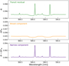 |
Fig. 1 Decomposition of the residual spectrum into broad and narrow components. The top panel is the transit residual, R, that can be calculated following Eq. (1). This is further split into the broad component (middle orange line) and the narrow component (bottom purple line). The broadened component is the out-of-transit stellar spectrum scaled by the transit depth, DF*. The narrow component is the difference between the transit residual spectrum and the broadened component. |
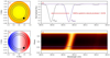 |
Fig. 2 (Movie online) Model isolated spectrum from a single in-transit exposure of WASP-189 b at phase ϕ = −0.018. The spectrum has been cropped to show a single line of the Na doublet. Subfigures (a) and (b) show the position of the transiting planet at the current phase as a solid black circle over the star. The annulus of similar stellar composition is also indicated in these figures with solid black lines. The colour of the star in (a) represents limb-darkening, and (b) represents the rotation of the star, with the respective blue and red Doppler shifts. Subfigure (c) shows the momentary local obscured spectrum, Fobsc, in purple and the isolated spectrum, F*,N, with the dashed black line. (d) contains the time-series in-transit residuals, R, with the horizontal purple line indicating the current planetary orbital phase. The colours represent the flux level, with a greater flux being more yellow and a lower flux being darker. It is important to note that this residual spectrum is different from the extracted non-broadened spectrum above. |
2.3 Flux calibration and continuum normalisation
The theory described above assumes that the spectral time series is flux calibrated. In reality, ground-based observations may be arbitrary scaled and vary in flux, so in real analyses, a normalisation is typically applied to F(t). To ensure that Eq. (6) holds in such cases, we carried out a rescaling of F(t) by dividing out the mean of the spectrum, ![Mathematical equation: $\[\bar{F}(t)\]$](/articles/aa/full_html/2024/11/aa50624-24/aa50624-24-eq12.png) , to obtain the normalised spectrum; and then by reintroducing the broadband limb-darkened light curve into the normalised time series. This follows the established practice when extracting obscured stellar line residuals (see e.g. Cegla et al. 2016). The observed residual R′ are in the form
, to obtain the normalised spectrum; and then by reintroducing the broadband limb-darkened light curve into the normalised time series. This follows the established practice when extracting obscured stellar line residuals (see e.g. Cegla et al. 2016). The observed residual R′ are in the form
![Mathematical equation: $\[R^{\prime}=\frac{(1-D) F(t)}{F_{\mathrm{oot}}} \frac{\bar{F}_{\mathrm{oot}}}{\bar{F}(t)}.\]$](/articles/aa/full_html/2024/11/aa50624-24/aa50624-24-eq13.png) (11)
(11)
In the theoretical case of flux-calibrated spectra, ![Mathematical equation: $\[\frac{\bar{F}(t)}{\bar{F}_{\text{oot}}}\]$](/articles/aa/full_html/2024/11/aa50624-24/aa50624-24-eq14.png) is trivially equal to 1 − D, while in the case of real observations, the spectra F are scaled by an arbitrary continuum function α(λ) (e.g. because of instrumental throughput). Here that was divided out and it disappears.
is trivially equal to 1 − D, while in the case of real observations, the spectra F are scaled by an arbitrary continuum function α(λ) (e.g. because of instrumental throughput). Here that was divided out and it disappears.
Additionally, spectral synthesis methods require the characterisation of a spectral continuum to reliably fit photospheric lines. Using our method, continuum normalisation can be applied to the final isolated spectrum, F*,N. This bypasses the problem of continuum normalisation with a rotation-broadened spectrum, where severe line blending makes selecting continuum points for normalisation practically impossible (see Fig. 3). The term ![Mathematical equation: $\[\frac{1{-}R}{D}\]$](/articles/aa/full_html/2024/11/aa50624-24/aa50624-24-eq15.png) in Eq. (7) is approximately unity in the continuum. Therefore, by multiplying with the broadened out-of-transit stellar spectrum F*, the continuum of the obscured spectrum is scaled to the continuum level of F* – even if this continuum is not observed due to line blends (see Fig. 1).
in Eq. (7) is approximately unity in the continuum. Therefore, by multiplying with the broadened out-of-transit stellar spectrum F*, the continuum of the obscured spectrum is scaled to the continuum level of F* – even if this continuum is not observed due to line blends (see Fig. 1).
An additional refinement of the continuum normalisation may need to be applied to Fobsc by dividing by the median to ensure the weighted average (Eq. (10)) is unbiased; however, because the continuum of ![Mathematical equation: $\[\frac{1{-}R}{D}\]$](/articles/aa/full_html/2024/11/aa50624-24/aa50624-24-eq16.png) is close to one, any errors introduced in this way are very small. We could thus proceed to apply typical continuum normalisation methods to F*,N instead of F*.
is close to one, any errors introduced in this way are very small. We could thus proceed to apply typical continuum normalisation methods to F*,N instead of F*.
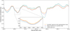 |
Fig. 3 Example segment of the mean out-of-transit stellar spectrum of WASP-189 from 3 nights of simulated HARPS observations (orange) with its best-fit spectrum (purple). The real HARPS spectrum (green) has been included to show how the synthetically generated spectrum compares. |
2.4 Fitting
We used the inbuilt fitting function in PySME to obtain best-fit photospheric parameters using the isolated stellar spectrum, F*,N, as extracted above using the line list extracted from VALD (see Sect. 2.2). The solver minimises the least-square error between the input spectrum and the spectrum as modelled by PySME for specified free parameters, Teff, log g, and [Fe/H], and individual chemical abundances. The fitting process uses the SciPy dogbox algorithm (Voglis & Lagaris 2004; Virtanen et al. 2020), which uses minimal function evaluations for convergence (Wehrhahn et al. 2023). This fitting algorithm was applied to the mean out-of-transit spectrum (consistent with methods in Prinoth et al. 2022), as well as the derived F*,N, and also a synthetic spectrum with no rotation broadening. As well as the photospheric parameters, we were interested in fitting the α element abundances of Mg, Ca, and Ti. The α element abundances are a metric often used in Galactic chemical evolution models to classify stellar populations (Matteucci & Brocato 1990), and thus they are an interesting measure to provide beyond determining the stellar parameters. Furthermore, for future retrieval work on WASP-189 b, there is a need to know the stellar abundances for comparison with retrieved planetary abundances.
The fitting process was as follows:
Before fitting the photospheric parameters, we performed a sensitivity analysis to determine which lines in the spectrum are more sensitive to variations of global parameters, Teff, log g, [Fe/H], and υ sin i*, and, separately, individual elemental abundances. The latter was achieved by fixing the global parameters and synthesising new spectra with chemical abundances varying by ±0.2 dex.
Segments of approximately 0.5–3 nm containing the most sensitive lines were selected for both the global parameters as well as for each elemental abundance. Regions where sensitive lines were strongly blended were discarded. In this way, 26 segments were selected to fit the global parameters, while individual species were fit using varying number of segments depending on the location of their strongest lines.
For each selected segment, masks were created by manually selecting the wavelength regions containing the target lines (see Fig. 4). In this way, 66 masks over the entire spectrum containing 191 Fe lines (see Table A.1) were selected to fit the global parameters. Separate continuum masks were also created to allow PySME to fit the arbitrary continuum level as described in Sect. 2.3.
We conducted a fit to determine the optimal values of the global parameters, Teff, log g, [Fe/H], and υ sin i* from the extracted F*,N as well as their uncertainties.
With global parameters Teff, log g, and υ sin i* fixed to their best-fit values, the selected lines were used to fit individual abundances separately.
To estimate the systematic errors on individual abundances introduced by fixing the global parameters, we varied Teff and log g by their uncertainties (see point 3). This yielded noise terms σT and σg that we added in squares to the statistical uncertainty, σn, reported by PySME:
![Mathematical equation: $\[\sigma_T^2+\sigma_g^2+\sigma_n^2\]$](/articles/aa/full_html/2024/11/aa50624-24/aa50624-24-eq17.png) . It is important to note that σn is usually small compared to the other terms.
. It is important to note that σn is usually small compared to the other terms.
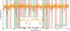 |
Fig. 4 Example segment of the average isolated stellar spectrum, F*,N, from three WASP-189 b transits from a simulated HARPS observation (orange) with its best-fit spectrum (purple). The green shaded regions mark the pixels used for fitting various parameters and abundances. The red regions mark the pixels used for continuum fitting. |
3 WASP-189: Proof of concept
Throughout this paper, we have used, as an example, the A-type star WASP-189 and its ultra-hot Jupiter WASP-189 b. The exoplanet was discovered by Anderson et al. (2018) with the WASP-South survey and TRAPPIST-South telescope, and confirmed with RV and Doppler tomography observations using HARPS and CORALIE spectrographs. This star is an ideal candidate to study with our method as it is a very bright (MV = 6.6 mag) fast rotator with a high projected rotational velocity υ sin i* = 93.1 km/s (Lendl et al. 2020). Since its discovery in 2018, transits have been observed repeatedly with spectrographs (e.g. Prinoth et al. 2023). As a proof of concept, we created a synthetic model of these observed time-series spectral observations using the method as described in Sect. 2.1.
The signal-to-noise ratio (S/N) and wavelength range for the synthetically generated spectra were designed to match WASP-189 b transit spectra observed with the HARPS spectrograph (Mayor et al. 2003). HARPS has a S/N of 110 at 550 nm for a MV = 6 star observed for 1 minute and covers a wavelength range of 378–5691 nm over 72 spectral orders with a spectral resolution of 115 000. To ensure the calculation of the weighted average following Eq. (10) matches real transit spectra, the phases of each observation were taken to be the same as each night of HARPS observations in Prinoth et al. (2023).
Following the method described in Sect. 2.1, the stellar and planetary parameters from Table 1 were used as input for StarRotator and PySME to interpolate spectra from a given model atmosphere and henceforth to simulate the time-series synthetic spectra as observed with HARPS at the three epochs as stated in Prinoth et al. (2023). The S/N values were estimated for each epoch from real time series spectral observations in wavelength and time. Random Gaussian noise with a standard deviation corresponding to this S/N was added to each synthetic spectrum to mimic a real exposure.
We required the RV of the stellar disc directly behind the transiting planet to shift the spectra to the rest frame (see Eq. (8)). StarRotator computed the RVs over the stellar disc using a grid-based approach. The obscured spectra were shifted by the mean velocity of the grid cells blocked by the exoplanet.
The transit light curve from StarRotator was calculated based on radiative transfer equations within PySME and not any specific limb-darkening law. However, to calculate the transit depth, D, with Eq. (3), we required the limb-darkening coefficients u1 and u2. We therefore obtained the limb-darkening coefficients by fitting the quadratic limb-darkening model to the light curve obtained using StarRotator, using NumPyro (Bingham et al. 2019; Phan et al. 2019) and Jax (Bradbury et al. 2018). The fitted parameters are listed in Table 2, and are broadly consistent with the measured values from Deline et al. (2022).
Figure 3 shows the mean out-of-transit-broadened stellar spectrum of WASP-189, which would usually be used to fit photospheric parameters. We carried out a fit of the broadened out-of-transit spectrum using PySME (see Sect. 2.4) and due to the high S/N, the measurements were precise. However, the fitted values were systematically offset (see Table 3 and Fig. 3). This is because continuum points are difficult to identify within a wavelength segment, affecting continuum fitting and introducing significant errors when fitting lines of the significantly rotation-broadened (υ sin i* ≈ 100 km/s) spectrum as all the lines are blended, skewing the results of the fitted spectrum – even for a fully synthetically modelled spectrum.
On the other hand, the isolated spectrum, F*,N, shows clear spectral lines and a flat continuum level, however at a cost of decreased S/N (see Fig. 4), which is the main limitation of our method. From a single transit observation of WASP-189 b with HARPS, the S/N of F*,N was approximately 5. This increases to approximately 10, for three stacked transits. When fitting the photospheric parameters, the statistical uncertainties were increased; however, the results were more accurate.
To determine how well we can fit the isolated spectrum in an ideal scenario with decreased noise, we conducted a separate analysis where we varied the noise added to the synthetic isolated spectrum, F*,N. We added random Gaussian noise with a S/N of 10, 20, 30, 40, and 50 to obtain datasets of the same spectrum with varying noise levels. This was repeated ten times to produce a spread of datasets with different realisations of random Gaussian noise, but with the same S/N. Following the same fitting procedure as in Sect. 2.4, the results for the global parameters Teff, log g, and [Fe/H] are presented in Fig. 5, including the spread from fitting each of the ten datasets with the same S/N. The best-fit parameters were observed to converge to the true value at a higher S/N ≈ 40 (see Fig. 5). This indicates that with a sufficiently high S/N, it is possible to use the isolated spectrum, F*,N, to fit photospheric parameters with an increased accuracy and reliability compared to the out-of-transit stellar spectrum with a rotation broadening of υeq = 96.163 km/s.
Input WASP-189 system parameters used to generate the synthetic spectrum with StarRotator.
Fitted limb-darkening coefficients to light curve generated with modelled spectra including centre-to-limb variation from PySME.
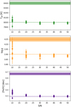 |
Fig. 5 Fitted global photospheric parameters (Teff, log g, and [Fe/H], from top to bottom) of the true synthetic isolated spectrum, F*,N, with a varying S/N. The horizontal dashed line is the true value of the corresponding parameter. The horizontal shaded region is the fitted result from the synthetic-broadened fit. |
4 Results
Best-fit parameters to the stellar spectra, F* (broadened and non-broadened), as well as the isolated spectra, F*,N, derived from the synthetic data are shown in Table 3 (see also Sect. 2.4). Fits to broadened stellar lines converge to systematically deviant values, but fits to the isolated spectrum can more accurately fit these parameters. The reported uncertainties are solely based on the least-squares algorithm used by PySME to fit the spectra, and do not take into account correlations between parameters. We therefore carried out these fits several times, for varying S/Ns, to demonstrate that statistically, the best-fit parameters converge to the true input values of the generated model (see Fig. 5).
In addition to testing our method with synthetic models, we also isolated the narrow stellar spectrum of WASP-189 from real HARPS observations previously published in Prinoth et al. (2023) (see Fig. 6). We obtained best-fit parameters shown in Table 4, with the best-fit spectrum overplotted in Fig. 6. Two separate abundance fits were performed: first fixing Teff and log g to the fitted parameters from a global fit on the same isolated spectrum, and another fixing Teff and log g to literature values reported by Lendl et al. (2020). Fixing Teff and log g to independently measured values is expected to be the strongest use case for the method we present here: Such parameters will generally become available from other photometric or spectroscopic measurements. As a result, accurate measurements of the abundances of individual elements can be obtained more reliably than from the rotation-broadened spectrum. This is because the isolated spectrum, F*,N, exhibits significantly fewer lines blending and a more identifiable continuum level, allowing lines of target elements to be fit more accurately.
When fixing Teff and log g to the values measured by Lendl et al. (2020), we find a metallicity of 0.50 ± 0.05 dex. This means that our measurement indicates that WASP-189 is a metal-rich star, with a higher metallicity than previously reported (0.29 ± 0.13 dex, Lendl et al. 2020). Figure 6 shows a comparison between our measured metallicity of [Fe/H] = 0.5 dex with model spectra varying [Fe/H] by ±0.2 dex. This shows that despite the relatively high noise level, PySME is able to converge robustly. This measured metallicity is consistent with expectations that metal-rich stars are more likely to host gas giants (Fischer & Valenti 2005).
Not only did we measure a new value for the metallicity of WASP-189, but we were also able to fit abundances of other elements. As a proof of concept, we focused on measuring the abundances of α elements Mg, Ca, and Ti. We report the abundances of these elements in Table 4. The individual chemical abundances for α elements we report are also consistent with previous surveys, reporting that high metallicity stars have less α enhancement (Buder et al. 2021).
Previous studies struggled to reliably determine abundances of fast-rotating stars due to extreme line blending, making it difficult to identify lines of target species (e.g. Ansari 1992; Takeda et al. 2009). This difficulty applies to all methods used to fit abundances, including spectral line fitting and equivalent width calculations. Takeda et al. (2009) stated that the reported abundances for the fast rotators (υ sin i* ⪆ 100 km/s) in their study are unreliable due to the lack of unblended lines available for fitting. By isolating the stellar spectrum with the help of an exoplanet companion, we prove that many more lines can be accessed (see Fig. 4 and Table A.1). A fitting method of the user’s choice can then be applied to the isolated spectrum, F*,N.
When fitting υ sin i* to real observational data, we report an increased value compared to the synthetic case. This additional broadening of υ sin i* ≈ 3 km/s is likely due to other effects such as spectrograph line spread functions being absorbed into the total υ sin i*. The instrument’s exposure time also introduces blurring from the planet moving across the stellar disc, broadening the spectrum by a few km/s.
Our method is limited by the S/N of current observations. The isolated stellar spectrum, F*,N, has a significantly lower S/N than the mean out-of-transit-broadened spectrum (see Fig. 4). This limits how precisely we could measure stellar abundances. High-resolution spectrographs on bigger telescopes (e.g. ANDES on the ELT) will enable observations of F*,N at higher S/Ns, leading to much smaller uncertainties on the photospheric parameters and elemental abundances (see Fig. 5), making this method of isolating the stellar spectrum potentially very powerful in the future. This study was limited to three available HARPS observations, but more in-transit observations of the target star will also help to improve the final S/N. Thus, if provided with a few time-series spectra of a sufficient S/N, it will be beneficial to apply our method of isolating the narrow stellar spectrum to measure individual chemical abundances.
Results from the fitted model of synthetic spectra of WASP-189 compared with the input parameters.
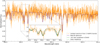 |
Fig. 6 Average isolated spectrum, F*,N, calculated from three real HARPS transits (orange) and its corresponding best-fit spectrum (purple) with Teff and log g fixed to parameters from Lendl et al. (2020). The shaded green region in the inset indicates ±0.2 variations in metallicity, [Fe/H]. The dotted green line indicates the spectrum with solar metallicity, [Fe/H] = 0. |
Fitted results for WASP-189 from three stacked transits observed with HARPS.
5 Conclusions
Line blending in rotation-broadened stellar spectra poses a problem when trying to measure the photospheric properties and individual chemical abundances in fast-rotating A-type stars. In this work, we have presented a new method to isolate the non-broadened stellar spectrum from the flux obscured by a transiting exoplanet, commonly referred to as the Doppler shadow. This spectrum, F*,N, is isolated from transit spectral time-series observations, and allows fitting photospheric parameters using standard spectral synthesis methods. We have demonstrated our proof of concept using synthetic spectra of WASP-189 generated with PySME and StarRotator. We have shown that even at the expense of a decreased S/N, the narrow isolated spectrum, F*,N, has a much more identifiable continuum level and less severe line blending, allowing us to more precisely measure stellar abundances.
We have applied this method to real observational data from the combination of three transits observed by the HARPS spectrograph, measuring higher metal abundances than previously reported by Lendl et al. (2020). With instruments with an improved S/N, such as the MAROON-X spectrograph on Gemini North or larger telescopes, or by using spectra from additional transit events, it will be possible to more tightly constrain these values.
These higher precision stellar abundances have important implications for the study of ultra-hot Jupiters, which tend to orbit young fast-rotating A-type host stars. Knowing the composition of the host star more precisely will allow for more reliable transmission spectroscopy for hot Jupiters, which will ultimately be used to understand the formation and evolution mechanisms involved in these systems, based on how the composition of the planet compares to the composition of the host star. This method can be applied to other hot Jupiter systems, such as KELT-9, MASCARA-2, or MASCARA-4, or to other systems involving fast-rotating stars and a companion that partially obscures the stellar disc during a transit event.
Data availability
The movie associated to Fig. 2 is available at https://www.aanda.org
Acknowledgements
M.L. acknowledges financial support from the Lund Global Scholarship and the Eleanor Sophia Wood Postgraduate Research Travelling Scholarship. B.P. acknowledges financial support from The Fund of the Walter Gyllenberg Foundation. B.T. acknowledges the financial support from the Wenner-Gren Foundation (WGF2022-0041). This work is based in part on observations collected at the European Southern Observatory under ESO programme 107.22QF. This research has made use of the services of the ESO Science Archive Facility.
Appendix A Line selection
Line data for Fe.
Line data for Ca.
Line data for Mg.
Line data for Ti.
References
- Abt, H. A. 2000, ApJ, 544, 933 [NASA ADS] [CrossRef] [Google Scholar]
- Adelman, S. J. 1973, ApJ, 183, 95 [NASA ADS] [CrossRef] [Google Scholar]
- Adelman, S. J., & Gulliver, A. F. 1990, ApJ, 348, 712 [NASA ADS] [CrossRef] [Google Scholar]
- Albrecht, S., Reffert, S., Snellen, I., Quirrenbach, A., & Mitchell, D. S. 2007, A&A, 474, 565 [NASA ADS] [CrossRef] [EDP Sciences] [Google Scholar]
- Albrecht, S., Winn, J. N., Johnson, J. A., et al. 2012, ApJ, 757, 18 [NASA ADS] [CrossRef] [Google Scholar]
- Anderson, D. R., Temple, L. Y., Nielsen, L. D., et al. 2018, arXiv e-prints [arXiv:1809.04897] [Google Scholar]
- Ansari, S. G. 1992, A&A, 259, 211 [NASA ADS] [Google Scholar]
- Asplund, M., Grevesse, N., Sauval, A. J., & Scott, P. 2009, ARA&A, 47, 481 [NASA ADS] [CrossRef] [Google Scholar]
- Bingham, E., Chen, J. P., Jankowiak, M., et al. 2019, J. Mach. Learn. Res., 20, 28 [Google Scholar]
- Borgniet, S., Lagrange, A. M., Meunier, N., & Galland, F. 2017, A&A, 599, A57 [NASA ADS] [CrossRef] [EDP Sciences] [Google Scholar]
- Bourrier, V., Ehrenreich, D., Lendl, M., et al. 2020, A&A, 635, A205 [NASA ADS] [CrossRef] [EDP Sciences] [Google Scholar]
- Bowler, B. P., Johnson, J. A., Marcy, G. W., et al. 2010, ApJ, 709, 396 [Google Scholar]
- Bradbury, J., Frostig, R., Hawkins, P., et al. 2018, JAX: composable transformations of Python+NumPy programs [Google Scholar]
- Buchhave, L. A., Bizzarro, M., Latham, D. W., et al. 2014, Nature, 509, 593 [Google Scholar]
- Buder, S., Sharma, S., Kos, J., et al. 2021, MNRAS, 506, 150 [NASA ADS] [CrossRef] [Google Scholar]
- Casasayas-Barris, N., Pallé, E., Yan, F., et al. 2018, A&A, 616, A151 [NASA ADS] [CrossRef] [EDP Sciences] [Google Scholar]
- Cauley, P. W., & Ahlers, J. P. 2022, AJ, 163, 122 [NASA ADS] [CrossRef] [Google Scholar]
- Cegla, H. M., Lovis, C., Bourrier, V., et al. 2016, A&A, 588, A127 [NASA ADS] [CrossRef] [EDP Sciences] [Google Scholar]
- Collier Cameron, A., Guenther, E., Smalley, B., et al. 2010, MNRAS, 407, 507 [NASA ADS] [CrossRef] [Google Scholar]
- Csizmadia, S., Pasternacki, T., Dreyer, C., et al. 2013, A&A, 549, A9 [NASA ADS] [CrossRef] [EDP Sciences] [Google Scholar]
- Cumming, A., Butler, R. P., Marcy, G. W., et al. 2008, PASP, 120, 531 [CrossRef] [Google Scholar]
- Deline, A., Hooton, M. J., Lendl, M., et al. 2022, A&A, 659, A74 [NASA ADS] [CrossRef] [EDP Sciences] [Google Scholar]
- Dravins, D., Ludwig, H.-G., Dahlén, E., & Pazira, H. 2017, A&A, 605, A90 [NASA ADS] [CrossRef] [EDP Sciences] [Google Scholar]
- Fischer, D. A., & Valenti, J. 2005, ApJ, 622, 1102 [NASA ADS] [CrossRef] [Google Scholar]
- Galland, F., Lagrange, A. M., Udry, S., et al. 2005, A&A, 443, 337 [NASA ADS] [CrossRef] [EDP Sciences] [Google Scholar]
- Gaudi, B. S., Stassun, K. G., Collins, K. A., et al. 2017, Nature, 546, 514 [NASA ADS] [Google Scholar]
- Gigas, D. 1986, A&A, 165, 170 [Google Scholar]
- Glebocki, R., & Gnacinski, P. 2005, VizieR On-line Data Catalog: III/244 [Google Scholar]
- Gray, R. O., & Garrison, R. F. 1987, ApJS, 65, 581 [NASA ADS] [CrossRef] [Google Scholar]
- Grevesse, N., Asplund, M., & Sauval, A. J. 2007, Space Sci. Rev., 130, 105 [Google Scholar]
- Hartman, J. D., Bakos, G. Á., Buchhave, L. A., et al. 2015, AJ, 150, 197 [NASA ADS] [CrossRef] [Google Scholar]
- Hill, G., Gulliver, A. F., & Adelman, S. J. 2004, IAU Symp., 224, 35 [NASA ADS] [Google Scholar]
- Hoeijmakers, H. J., Seidel, J. V., Pino, L., et al. 2020, A&A, 641, A123 [NASA ADS] [CrossRef] [EDP Sciences] [Google Scholar]
- Johnson, J. A., Fischer, D. A., Marcy, G. W., et al. 2007, ApJ, 665, 785 [Google Scholar]
- Johnson, J. A., Clanton, C., Howard, A. W., et al. 2011, ApJS, 197, 26 [Google Scholar]
- Kipping, D. M. 2013, MNRAS, 435, 2152 [Google Scholar]
- Kurucz, R. L. 1993, ASP Conf. Ser., 44, 87 [Google Scholar]
- Lendl, M., Csizmadia, S., Deline, A., et al. 2020, A&A, 643, A94 [EDP Sciences] [Google Scholar]
- Lothringer, J. D., Rustamkulov, Z., Sing, D. K., et al. 2021, ApJ, 914, 12 [CrossRef] [Google Scholar]
- Matteucci, F., & Brocato, E. 1990, ApJ, 365, 539 [CrossRef] [Google Scholar]
- Mayor, M., Pepe, F., Queloz, D., et al. 2003, The Messenger, 114, 20 [NASA ADS] [Google Scholar]
- McLaughlin, D. B. 1924, ApJ, 60, 22 [Google Scholar]
- Phan, D., Pradhan, N., & Jankowiak, M. 2019, arXiv eprint [arXiv:1912.11554] [Google Scholar]
- Piskunov, N., & Valenti, J. A. 2017, A&A, 597, A16 [NASA ADS] [CrossRef] [EDP Sciences] [Google Scholar]
- Piskunov, N. E., Kupka, F., Ryabchikova, T. A., Weiss, W. W., & Jeffery, C. S. 1995, A&AS, 112, 525 [Google Scholar]
- Preston, G. W. 1974, ARA&A, 12, 257 [Google Scholar]
- Prinoth, B., Hoeijmakers, H. J., Kitzmann, D., et al. 2022, Nat. Astron., 6, 449 [NASA ADS] [CrossRef] [Google Scholar]
- Prinoth, B., Hoeijmakers, H. J., Pelletier, S., et al. 2023, A&A, 678, A182 [NASA ADS] [CrossRef] [EDP Sciences] [Google Scholar]
- Prinoth, B., Hoeijmakers, H. J., Morris, B. M., et al. 2024, A&A, 685, A60 [NASA ADS] [CrossRef] [EDP Sciences] [Google Scholar]
- Rossiter, R. A. 1924, ApJ, 60, 15 [Google Scholar]
- Royer, F., Gebran, M., Monier, R., et al. 2014, A&A, 562, A84 [NASA ADS] [CrossRef] [EDP Sciences] [Google Scholar]
- Ryabchikova, T., Piskunov, N., Kurucz, R. L., et al. 2015, Phys. Scr, 90, 054005 [Google Scholar]
- Santos, N. C., Israelian, G., & Mayor, M. 2004, A&A, 415, 1153 [NASA ADS] [CrossRef] [EDP Sciences] [Google Scholar]
- Sato, B., Omiya, M., Harakawa, H., et al. 2012, PASJ, 64, 135 [Google Scholar]
- Schulze, J. G., Wang, J., Johnson, J. A., et al. 2021, PSJ, 2, 113 [Google Scholar]
- Smith, K. C. 1996, Ap&SS, 237, 77 [NASA ADS] [CrossRef] [Google Scholar]
- Takeda, Y., Kang, D.-I., Han, I., Lee, B.-C., & Kim, K.-M. 2009, PASJ, 61, 1165 [NASA ADS] [Google Scholar]
- Unterborn, C. T., & Panero, W. R. 2017, ApJ, 845, 61 [NASA ADS] [CrossRef] [Google Scholar]
- Valenti, J. A., & Piskunov, N. 1996, A&AS, 118, 595 [NASA ADS] [CrossRef] [EDP Sciences] [Google Scholar]
- Virtanen, P., Gommers, R., Oliphant, T. E., et al. 2020, Nat. Methods, 17, 261 [Google Scholar]
- Voglis, C., & Lagaris, I. 2004, in WSEAS International Conference on Applied Mathematics, 7, 9780429081385-138 [Google Scholar]
- Wehrhahn, A., Piskunov, N., & Ryabchikova, T. 2023, A&A, 671, A171 [NASA ADS] [CrossRef] [EDP Sciences] [Google Scholar]
- Winn, J. N. 2010, in Exoplanets, ed. S. Seager (Tucson, AZ: University of Arizona Press), 55 [Google Scholar]
- Winn, J. N., Fabrycky, D., Albrecht, S., & Johnson, J. A. 2010, ApJ, 718, L145 [Google Scholar]
- Yan, F., Pallé, E., Fosbury, R. A. E., Petr-Gotzens, M. G., & Henning, T. 2017, A&A, 603, A73 [NASA ADS] [CrossRef] [EDP Sciences] [Google Scholar]
Fp is not to be confused with the transmission spectrum of the atmosphere of the planet, which is not considered in this study.
Gravity darkening manifests itself as a temperature gradient from the stellar equator to the pole, breaking the point symmetry assumed in this formalism. For typical exoplanet hosts, this temperature gradient can be as high as 700 K (Cauley & Ahlers 2022), but this range would only be probed for planets with a zero impact parameter.
All Tables
Input WASP-189 system parameters used to generate the synthetic spectrum with StarRotator.
Fitted limb-darkening coefficients to light curve generated with modelled spectra including centre-to-limb variation from PySME.
Results from the fitted model of synthetic spectra of WASP-189 compared with the input parameters.
All Figures
|
Fig. 1 Decomposition of the residual spectrum into broad and narrow components. The top panel is the transit residual, R, that can be calculated following Eq. (1). This is further split into the broad component (middle orange line) and the narrow component (bottom purple line). The broadened component is the out-of-transit stellar spectrum scaled by the transit depth, DF*. The narrow component is the difference between the transit residual spectrum and the broadened component. |
| In the text | |
|
Fig. 2 (Movie online) Model isolated spectrum from a single in-transit exposure of WASP-189 b at phase ϕ = −0.018. The spectrum has been cropped to show a single line of the Na doublet. Subfigures (a) and (b) show the position of the transiting planet at the current phase as a solid black circle over the star. The annulus of similar stellar composition is also indicated in these figures with solid black lines. The colour of the star in (a) represents limb-darkening, and (b) represents the rotation of the star, with the respective blue and red Doppler shifts. Subfigure (c) shows the momentary local obscured spectrum, Fobsc, in purple and the isolated spectrum, F*,N, with the dashed black line. (d) contains the time-series in-transit residuals, R, with the horizontal purple line indicating the current planetary orbital phase. The colours represent the flux level, with a greater flux being more yellow and a lower flux being darker. It is important to note that this residual spectrum is different from the extracted non-broadened spectrum above. |
| In the text | |
|
Fig. 3 Example segment of the mean out-of-transit stellar spectrum of WASP-189 from 3 nights of simulated HARPS observations (orange) with its best-fit spectrum (purple). The real HARPS spectrum (green) has been included to show how the synthetically generated spectrum compares. |
| In the text | |
|
Fig. 4 Example segment of the average isolated stellar spectrum, F*,N, from three WASP-189 b transits from a simulated HARPS observation (orange) with its best-fit spectrum (purple). The green shaded regions mark the pixels used for fitting various parameters and abundances. The red regions mark the pixels used for continuum fitting. |
| In the text | |
|
Fig. 5 Fitted global photospheric parameters (Teff, log g, and [Fe/H], from top to bottom) of the true synthetic isolated spectrum, F*,N, with a varying S/N. The horizontal dashed line is the true value of the corresponding parameter. The horizontal shaded region is the fitted result from the synthetic-broadened fit. |
| In the text | |
|
Fig. 6 Average isolated spectrum, F*,N, calculated from three real HARPS transits (orange) and its corresponding best-fit spectrum (purple) with Teff and log g fixed to parameters from Lendl et al. (2020). The shaded green region in the inset indicates ±0.2 variations in metallicity, [Fe/H]. The dotted green line indicates the spectrum with solar metallicity, [Fe/H] = 0. |
| In the text | |
Current usage metrics show cumulative count of Article Views (full-text article views including HTML views, PDF and ePub downloads, according to the available data) and Abstracts Views on Vision4Press platform.
Data correspond to usage on the plateform after 2015. The current usage metrics is available 48-96 hours after online publication and is updated daily on week days.
Initial download of the metrics may take a while.