| Issue |
A&A
Volume 691, November 2024
|
|
|---|---|---|
| Article Number | A345 | |
| Number of page(s) | 16 | |
| Section | Extragalactic astronomy | |
| DOI | https://doi.org/10.1051/0004-6361/202450407 | |
| Published online | 25 November 2024 | |
New AGN diagnostic diagrams based on the [OIII]λ4363 auroral line
1
Dipartimento di Fisica e Astronomia, Università di Bologna, Via Gobetti 93/2, I-40129 Bologna, Italy
2
INAF – Osservatorio di Astrofisica e Scienza dello Spazio di Bologna, Via Gobetti 93/3, I-40129 Bologna, Italy
3
Kavli Institute for Cosmology, University of Cambridge, Madingley Road, Cambridge CB3 0HA, UK
4
Cavendish Laboratory, University of Cambridge, 19 JJ Thomson Avenue, Cambridge CB3 0HE, UK
5
Department of Physics and Astronomy, University College London, Gower Street, London WC1E 6BT, UK
6
National Astronomical Observatory of Japan, 2-21-1 Osawa, Mitaka, Tokyo 181-8588, Japan
7
INAF-Osservatorio Astrofisico di Arcetri, Largo E. Fermi 5, I-50125 Firenze, Italy
8
European Southern Observatory, Karl-Schwarzschild-Strasse 2, 85748 Garching, Germany
9
Dipartimento di Fisica e Astronomia, Università di Firenze, Via G. Sansone 1, I-50019 Sesto F.no (Firenze), Italy
⋆ Corresponding author; This email address is being protected from spambots. You need JavaScript enabled to view it.
Received:
16
April
2024
Accepted:
25
July
2024
Abstract
The James Webb Space Telescope (JWST) is revolutionizing our understanding of black hole formation and growth in the early Universe. However, JWST has also revealed that some of the classical diagnostics, such as the Baldwin, Phillips & Terlevich (BPT) diagrams and X-ray emission, often fail to identify active galactic nuclei (AGN) at high redshift and low metallicity. Here we present three new rest-frame optical diagnostic diagrams to identify narrow-line Type II AGN, leveraging the [OIII]λ4363 auroral line, which has been detected in several JWST spectra. Specifically, we show that high values of the [OIII]λ 4363 / Hγ ratio provide a sufficient (but not necessary) condition to identify the presence of an AGN, based on empirical calibrations (using local and high-redshift sources) and on a broad range of photoionization models. These diagnostics are able to separate much of the AGN population from star-forming galaxies (SFGs): the average energy of an AGN’s ionizing photons is higher than that of young stars in SFGs, and hence AGN can more efficiently heat the gas, thus boosting the [OIII]λ4363 line. We also found independent indications of AGN activity in some high-redshift sources (z > 4) that were not previously identified as AGN with the traditional diagnostics diagrams, but that are placed in the AGN region of the diagnostic presented in this work. We note, conversely, that low values of [OIII]λ 4363 / Hγ can be associated either with SFGs or AGN excitation. We note that the fact that strong auroral lines are often associated with AGN does not imply that they cannot be used for direct metallicity measurements (provided that proper ionization corrections are applied), but it does affect the calibration of strong line metallicity diagnostics.
Key words: galaxies: active / galaxies: high-redshift / galaxies: ISM
© The Authors 2024
 Open Access article, published by EDP Sciences, under the terms of the Creative Commons Attribution License (https://creativecommons.org/licenses/by/4.0), which permits unrestricted use, distribution, and reproduction in any medium, provided the original work is properly cited.
This article is published in open access under the Subscribe to Open model. This email address is being protected from spambots. You need JavaScript enabled to view it. to support open access publication.
1. Introduction
Thanks to the successful launch of the James Webb Space Telescope (JWST; Gardner et al. 2023; Rigby et al. 2023), we can now investigate with high resolution and unprecedented sensitivity both the photometric and spectroscopic properties of galaxies up to z ∼ 13 (Curtis-Lake et al. 2022; Robertson et al. 2022). Within this context, recent studies exploiting different kinds of JWST data have revealed a large population of AGN at high redshift (Kocevski et al. 2023; Übler et al. 2023; Matthee et al. 2023; Maiolino et al. 2024b,c; Greene et al. 2023; Bogdán et al. 2023; Goulding et al. 2023; Kokorev et al. 2023; Furtak et al. 2023; Juodžbalis et al. 2024b; Scholtz et al. 2023; Chisholm et al. 2024), suggesting a higher AGN fraction at z > 3 than previously expected. For instance, Yang et al. (2023), taking advantage of the JWST-MIRI photometry of the Cosmic Evolution Early Release Science Survey (CEERS; Finkelstein et al. 2022), investigated the AGN population using spectral energy distribution (SED) modelling, and found a black hole accretion rate density (BHARD) at z > 3, which was ∼0.5 dex higher than expected from previous X-ray studies (Vito et al. 2016, 2018). Maiolino et al. (2024c) and Harikane et al. (2023), by selecting broad-line AGN (BLAGN, or Type I) among NIRSpec spectra (Ferruit et al. 2022; Jakobsen et al. 2022), have also found significant AGN excess at z > 4 with respect to the AGN luminosity functions derived using X-ray data (Giallongo et al. 2019).
The X-ray emission, produced in AGN by inverse-Compton scattering of the UV photons coming from the supermassive black hole (SMBH) accretion disc, has traditionally been used to select AGN. Most of the high-z AGN selected using JWST spectroscopy lie in fields covered by some of the deepest X-ray observations ever performed, for example the 7Ms Chandra Deep Field South (CDFS) (Luo et al. 2017), Chandra Deep Field North (CDFN) (Xue et al. 2016), and AEGIS-XD (Nandra et al. 2015). However, most of these newly discovered high-z AGN lack any X-ray emission (e.g. Mazzolari et al., in prep., Scholtz et al. 2023; Übler et al. 2023; Maiolino et al. 2024a; Kocevski et al. 2023; Wang et al. 2024; Juodžbalis et al. 2024a), with only a very few exceptions (Goulding et al. 2023; Kovacs et al. 2024; Kocevski et al. 2023). This makes the picture even more difficult to interpret, and suggests different scenarios such as Compton-thick obscuration (Gilli et al. 2022) or intrinsic X-ray weakness (Simmonds et al. 2016).
The difficulties in selecting high-z AGN are even more important for Type II or narrow-line AGN (NLAGN). Different observational works have already demonstrated that some of the traditional well-known AGN emission-line diagnostic diagrams, such as the Baldwin, Phillips & Terlevich (BPT) diagram (Baldwin et al. 1981), are no longer effective in the high-z Universe (Maiolino et al. 2024c; Scholtz et al. 2023; Harikane et al. 2023; Kocevski et al. 2023; Übler et al. 2023; Groves et al. 2006). At high-z the environments are systematically more metal poor and the stellar populations are generally younger, increasing the ionization parameter (log U) of star-forming galaxies (SFG). This effect, on the one hand, makes SFGs move towards the AGN locus on the BPT; on the other hand the lower metallicity of the narrow-line region (NLR) of AGN makes the line ratios move towards and overlap with the star formation locus on these traditional diagnostic diagrams. The detection of high-ionization emission lines (e.g. N Vλ1242, [Ne IV]λ2424, [Ne V]λ3426) can still be considered a safe tracer for the presence of an AGN (Calabro et al. 2024; Cleri et al. 2023; Brinchmann 2023; Chisholm et al. 2024), but their detection is still difficult, even in the deepest JWST spectroscopic surveys such as the JWST Advanced Deep Extragalactic Survey (JADES, Bunker et al. 2024; Scholtz et al. 2023).
To have a clear picture of the AGN properties and demographics at high-z, it is therefore crucial to identify new AGN selection techniques. Thanks to the wide wavelength coverage (∼1 − 5μm) and sensitivity of JWST, it is now possible to have access to a plethora of rest-UV and optical emission lines in high-z galaxies that were not accessible before. Among these lines, multiple JWST spectra have revealed the detection of the [OIII]λ4363 line. In the metal-poor and highly ionized environments of many high-z galaxies, [OIII]λ4363 is the strongest auroral line, a collisionally excited emission line generated from higher energy levels compared to the typical nebular lines. Due to its faintness and proximity to the (generally) stronger Hγ line, before the launch of JWST it had been detected and studied almost only in galaxies at z < 2. Given its sensitivity to the gas temperature, this line has been extensively used in the local Universe to determine the metallicity of the interstellar medium (ISM) via the direct temperature method, which exploits the possibility of computing the metallicity by fixing the gas electron temperature derived from the ratio between the [OIII]λ4363 and the [OIII]λ5007 nebular lines (see e.g. the review by Maiolino & Mannucci 2019).
However, Brinchmann (2023) first noticed that the anomalously high [OIII]λ4363 emission in some of the early NIRSpec spectra at z∼8 could indicate the presence of an AGN. More recently, Übler et al. (2024) have suggested that a strong ratio between this line and the Hγ line could be a possible indicator of the presence of an AGN. In their work, by using JWST/NIRSpec Integral Field Spectroscopy (IFS) observations, they found a spatial correspondence between the AGN broad Hβ emission and the [OIII]λ4363 line emission. They also mention the possibility that the enhanced [OIII]λ4363 emission in correspondence of the AGN could be related to higher ISM temperatures driven by the AGN activity.
An enhancement of the [OIII]λ4363 emission in the presence of an AGN is qualitatively expected. AGN ionizing photons are more energetic than ionizing photons produced in star-forming regions on average, and hence they can heat the gas more effectively by depositing a larger amount of energy per unit photon. In this work we explore this scenario more quantitatively, with the ultimate goal of exploring the possibility of selecting AGN using the [OIII]λ4363 line through an observational–empirical approach and via photoionization models. As a result, we propose three new AGN diagnostic diagrams that can also be effective at high-z.
In Section 2 we present the local and high-z observational samples and the set of photoionization models considered to test the validity of the new diagnostic diagrams. In Section 3 we describe the new diagnostic diagrams based on the line ratio [OIII]λ4363/Hγ and the demarcation lines that can be used to separate the AGN population from SFGs. Lastly, in Section 4 we provide interpretations of why these diagnostics work, and we show indications of the AGN nature of some newly identified AGN using these diagnostics. We also discuss the implications of this work on the metallicity estimates based on the [OIII]λ4363 line and on the strong-line metallicity diagnostics.
2. Methods
We selected several AGN and SFG samples and two different sets of photoionization models to populate the diagnostic diagrams that we use to select AGN. All the observational samples described in the following (Sects. 2.1 and 2.2) are listed in Table 1.
2.1. Low-redshift samples
The sample of low-z SFGs is composed of both normal SFGs and also of the local analogues of high-z galaxies (i.e. local galaxies that show intrinsic properties similar to those observed in high-z galaxies), in terms of metallicities and emission lines ratios (e.g. Izotov et al. 2018, 2019, 2021). The Sloan Digital Sky Survey (SDSS) DR7 (Abazajian et al. 2009) gives the most numerous sample, mostly made of z < 0.7 galaxies. Starting from the whole catalogue provided by MPA/JHU, we considered only sources with a S/N > 5 in all the lines involved in the diagnostic diagrams we present: [OIII]λ4363, [OIII]λ5007, [Ne III]λ3869, [OII]λ3727, and Hγ. Then we distinguished between AGN and SFGs using the BPT diagram (Baldwin et al. 1981), taking the AGN demarcation line provided by Kewley et al. (2001) and after considering a further cut in S/N> 5 also in the Hα, Hβ, and [N II] lines. Furthermore, we excluded from the selection AGN classified in the SDSS catalogue as BLAGN since the catalogue does not provide separately the NL and BL components of the Balmer lines, and our diagnostics rely on the NL emission only. We also corrected all the lines for dust attenuation using the Calzetti et al. (2000) attenuation law. The final SDSS SFG (AGN) sample considered in this work contains ∼2300 (∼800) sources.
We identified several samples of local analogues of high-z galaxies with reported [OIII]λ4363 line fluxes. From Yang et al. (2017b) we took the sample of ‘blueberries’, which are 40 dwarf starburst galaxies with small sizes (< 1kpc), very high ionization values ([OIII]λ5007/[OII]λ3727 ∼ 10 − 60), and low metallicities (7.1 < 12 + log(O/H) < 7.8). They were selected from the SDSS DR12 at z < 0.05 and followed up spectroscopically using the MMT telescope. We also considered 43 ‘green pea’ galaxies from Yang et al. (2017a) (i.e. nearby SFG with strong [OIII]λ5007 emission line), two-thirds of which also show a strong Lyα emission.
We included in the local analogue sample a compilation of ∼490 local SFGs with low metallicities from different works: Izotov et al. (2006, 2018, 2019), Berg et al. (2012), Pustilnik et al. (2020), Pustilnik et al. (2021), Nakajima et al. (2022). All these samples were selected considering local sources followed up with different telescopes to be sensitive to the faint [OIII]λ4363 line, which allowed them to measure the galaxies’ metallicity via the direct method. The metallicities of these sources span the range 12 + log(O/H)∼6.9 − 8.9.
We also included the sample of 165 extreme emission line galaxies (EELG) reported in Amorín et al. (2015), selected from the zCOSMOS survey (Lilly et al. 2007) in the redshift range 0.11 < z < 0.93. These are very compact (r50 ∼ 1.3 kpc), low-mass (M* ∼ 107 − 1010 M⊙) galaxies characterized by specific star formation rates (sSFRs) above the main sequence for star-forming galaxies of the same stellar mass and redshift.
The local AGN sample comprises Type II AGN showing different features and selected for different aims. The most numerous AGN sample is represented by the SDSS sample mentioned above. We included the Dors et al. (2020) Type II AGN sample, selected from SDSS DR7 using multiple AGN diagnostic diagrams to guarantee a high purity and showing a range of metallicities between 8.0 < 12 + log(O/H) < 9.2.
The compilation of Type II AGN includes three sources presented in Seyfert (1943): NGC1068, NGC1275, and the core of NGC 4151. These spectra were obtained at the Mount Wilson Observatory and are among the first galaxies hosting active SMBH ever observed. These three sources clearly show the [OIII]λ4363 emission line in their spectra.
We considered the sources described in Perna et al. (2017), selected from SDSS z < 0.8 spectra associated with X-ray emission and showing outflows, which can be spectrally decomposed from the narrow-line and broad-line region (BLR) emission. We also added Type I and Type II AGN from the S7 survey (Dopita et al. 2015; Thomas et al. 2017), where 131 nearby AGN were primarily selected because of their radio-detection, and then followed-up using the WiFeS instrument at high resolution (R = 7000), which allows the faint [OIII]λ4363 line to be resolved. In Thomas et al. (2017) they provide the narrow components of the emission lines, already subtracting the broad component, if present.
The 35 AGN selected in Armah et al. (2021) are Type II AGN in the local Universe (z < 0.06) characterized by quite high metallicities (average metallicity 12 + log(O/H) = 8.55). These sources were selected by the authors to study the neon-to-oxygen abundance and its evolution with metallicity.
The last sample of local AGN is from the MOSFIRE Deep Evolution Field (MOSDEF) survey (Kriek et al. 2015), which targeted the rest-frame optical spectra of ∼1500 H-band-selected galaxies at 1.37 < z < 3.8. We took the full MOSDEF catalogue and selected only those sources with a [OIII]λ4363 line with a S/N > 5; then we distinguished between AGN and SFG using the BPT diagram. With these S/N cuts, we could identify only three sources, all classified as AGN. This indicates the difficulty in detecting such a faint line further than in the local Universe in the pre-JWST era.
For all the samples reported above we took dust-corrected fluxes from the works reported in Table 1.
2.2. High-redshift samples
The high-z samples of AGN and SFGs only comprise sources observed spectroscopically using JWST, the only instrument with enough resolution, sensitivity, and IR-coverage to detect and disentangle the [OIII]λ4363 line at z > 3. We considered the full publicly released sample of sources with a medium-resolution (MR, R = 1000) spectrum in the CEERS (PID: 1345; Finkelstein et al. 2022) and JADES (PID: 1210; Bunker et al. 2024) surveys. For JADES, we considered the emission line fluxes and the AGN selection described in Scholtz et al. (2023). Starting from a sample of 110 sources with MR spectroscopy, a reliable redshift, and sufficient wavelength coverage, the authors performed a NLAGN selection using multiple AGN rest-frame UV and optical diagnostic diagrams, finally selecting 28 reliable AGN candidates in the redshift range 1.8 < z < 9.4. The diagnostic diagrams involved in the selection include the BPTs (Baldwin et al. 1981; Veilleux & Osterbrock 1987), the CIVλλ1549, 51/CIII]λλ1907, 1909 versus CIII]λλ1907, 1909 / HeIIλ1640, and the detection of high-ionization emission lines such as [NeV]λ3420 [NeIV]λλ2422, 24, NVλλ1239, 42. To select NLAGN the authors considered in these diagnostics both demarcation lines already defined in the literature, while in other cases (such as the BPTs) they defined new demarcation lines derived considering the distribution of photoionization models (Gutkin et al. 2016; Feltre et al. 2016; Nakajima & Maiolino 2022). Of all the initial JADES sources, only 19 show a [OIII]λ4363 detection, 7 of which are AGN. We followed the same approach for the CEERS program: starting from 313 MR spectra published by the CEERS collaboration, we selected 217 sources with a reliable spectroscopic redshift, and we finally selected 52 AGN candidates (Mazzolari et al., in prep.). For this work, we considered 32 sources with the [OIII]λ4363 line detected among the CEERS sample, 4 of which already classified as AGN. From the same programmes, we also collected the BLAGN identified by Maiolino et al. (2024c) and Harikane et al. (2023) at z > 4.5, carefully checking for, and when necessary subtracting, the broad component of the Hγ line.
We further considered the three z ∼ 8 galaxies in the galaxy cluster SMACS J0723.3-7327, observed in the Early Release Observations (ERO) JWST programme (Pontoppidan et al. 2022) and analysed in Curti et al. (2023). Exploiting the [OIII]λ4363 line detections in the NIRSpec spectra, the authors measured metallicities ranging from extremely metal-poor (12 + log(O/H)∼7) to about one-third solar. Two of them were later identified as AGN in Brinchmann (2023), due to the presence of the high-ionization [Ne IV] emission line in one and based on the high ionization parameter (logU ∼ −1) of the other.
The sample of high-z sources presented in Nakajima et al. (2023) includes galaxies from three different early JWST programmes (CEERS, ERO, GLASS; Treu et al. 2022) at 6 < z < 9. We selected only the ten sources with the [OIII]λ4363 line detected, and we marked as BLAGN those that were selected based on their broad Hα line in Harikane et al. (2023). For the latter, we subtracted the broad Hγ component, if present.
We included in the high-z AGN sample the BLAGN reported in Übler et al. (2023) at z ∼ 5.55, whose JWST/NIRSpec Integral Field Spectrograph (IFS) observation shows very high ionization lines and low metallicity (one-fourth solar). We also included both the components of the dual AGN candidate at z ∼ 7.15 reported in Übler et al. (2024). For this source, thanks to IFS spectroscopy, the authors were able to study the displacement between the position of the Hβ broad-line region (BLR) and the strong [OIII]λ5007 emission line centroid, which were interpreted as the emissions coming from two distinct sources 620 pc apart from each other. Interestingly, the authors also found an almost perfect alignment between the [OIII]λ4363 emission line peak and the peak of the Hβ BLR, suggesting a correlation between the intensity of the [OIII]λ4363 line and the presence of an AGN.
We considered the BLAGN reported in Kokorev et al. (2023) at z = 8.50 from the JWST UNCOVER Treasury survey (Labbe et al. 2021), showing a robust Hβ broad component and an unprecedented black hole to host a galaxy mass of at least ∼30%. An even larger black hole to host galaxy mass ratio was more recently found in the z = 6.86 BLAGN analysed in Juodžbalis et al. (2024b), representing an extreme example of dormant SMBH at high-z. We also considered the z = 7.04 BLAGN, triply imaged and lensed by the galaxy cluster Abell2744-QSO1, reported by Furtak et al. (2023). This source is probably undergoing a phase of rapid SMBH growth and is also heavily obscured since the authors measured an AV ∼ 3 from the Balmer decrement. It should be noted that in all these Type I AGN cases (most of which actually type 1.5–1.9) the broad component of the Balmer lines is not detected in Hγ, and hence the narrow component of Hγ can be easily measured.
We added to our high-z sample the z = 6.1 extreme SFG reported in Topping et al. (2024). Using distinct UV transitions, the authors found an electron density  , a metal-poor ionized gas (i.e. 12 + log(O/H) = 7.43), and a logU ∼ −1 based on the ratio [OIII]λ5007/[OII]λ3727. The authors ultimately classified this source as a SFG, based on the ratios of the rest-UV emission lines, but they also found some indications of possible AGN activity, for example the broad Hα component accounting for ∼20% of the line flux.
We finally included in the sample GN-z11, an exceptionally luminous galaxy at z = 10.6. Its JWST spectrum reveals the presence of an AGN through the detection of semi-forbidden lines tracing very high densities (inconsistent with the ISM, but typical of the BLR), other transitions typical of AGN, fast outflows, ionization cones, and a larger Lyα halo, consistent with those seen in lower redshift quasars (Maiolino et al. 2024b,d; Scholtz et al. 2024).
2.3. Photoionization models
The observational data were compared with the results coming from two different sets of photoionization models. The first set of models was initially described in Gutkin et al. (2016) (for star formation) and in Feltre et al. (2016) (for narrow-line AGN emission), and updated with more recent stellar spectra and with a better description of AGN cloud microturbulence (Mignoli et al. 2019; Hirschmann et al. 2019; Vidal-García et al. 2024). The photoionization models were built using the Cloudy code (version c13.03) (Ferland et al. 2013) for star formation and AGN narrow-line regions, assuming a wide range of parameters. In particular, they consider gas metallicities (Z, where [O/H]=log(Z/Z⊙)) in the range 10−4 < Z < 0.07, ionization parameters of the ionizing source −4 < log U < −1, dust-to-metal ratios (0.1 < ξ < 0.5), hydrogen gas densities (102 < (nH/cm−3) < 104), different carbon-to-oxygen abundances (C/O), and two different initial mass functions (IMFs) for star formation models. For a complete list of the values of the different parameters, we refer to Table 1 in Feltre et al. (2016). These models include predictions for both the AGN and SFG populations; the main feature differentiating between the AGN and SFG models is the ionizing spectrum, which is the spectral energy distribution (SED) of the incident ionizing radiation, the first showing a harder radiation field.
As reported above, the photoionization models of Gutkin et al. (2016) and Feltre et al. (2016) cover a wide range of parameters and might actually include physical conditions rarely found in the general populations of galaxies and in the local analogues. For example, previous theoretical and observational studies have suggested a correlation between metallicity and the ionization parameter in SF regions (e.g. Dopita et al. 2006; Mingozzi et al. 2020; Ji & Yan 2022), which implies certain combinations of metallicities and ionization parameters should rarely, if ever, be observed in SF regions. Since the demarcation lines in the new diagrams we propose rely on both the observational data and photoionization models, we performed the following check to make sure that the part of the models with highly unphysical combinations of parameters does not impact our results.
We performed a likelihood analysis comparing the observed line ratios in our samples of SFG and those predicted by the SFG of Gutkin et al. (2016) in order to limit the inclusion of highly improbable or unphysical combinations of the parameters. This method has been adopted in making model-based inferences for local galaxies (e.g. Blanc et al. 2015; Mingozzi et al. 2020; Ji & Yan 2022).
We considered a total of three sets of line ratios, including [OIII]λ4363/Hγ, [OIII]λ5007/Hβ, and [OII]λλ3726, 3728/Hγ. The inclusion of collisionally excited lines from different ionization states of oxygen as well as recombination lines of hydrogen helps break the degeneracy between the metallicity and the ionization parameter in the models. Following the formalism of Blanc et al. (2015), we calculated the likelihood of each model given each data point, and combined the likelihood with a flat prior in the log space spanned by the metallicity and the ionization parameter to obtain the posterior distribution of these two parameters. From the posteriors, we obtained the weighted average metallicities and ionization parameters for all SFGs. We then selected a region in the metallicity-ionization parameter space not populated by the posteriors of our sample of SFGs. While the models of Gutkin et al. (2016) and Feltre et al. (2016) have a large set of parameters, we note that the primary drivers of the variations in the predicted line ratios are the metallicity and the ionization parameter. To verify this point, we repeated the above calculation for models with different IMFs, densities, dust-to-gas ratios, and carbon-to-oxygen abundance ratios, which generally resulted in a similar distribution in the metallicity–ionization parameter space. With these results, we adopted a conservative cut to select realistic SFG models based on the 16th percentile of the inferred distribution in the metallicity–ionization parameter space that produces the highest boundary1.
Our final cut removes the region of the SFG parameter space spanned by log (Z/Z⊙) and log U according to the following relations:
 (1)
(1)
and
 (2)
(2)
In Fig. A.1 we plot our fiducial cut together with the inferred distribution of the metallicities and ionization parameters for our selected SFGs based on different sets of models. The cut basically removes regions having very high ionization parameters and high metallicities at the same time. From a physical point of view, due to the dependence of the ionizing spectra of young stellar populations and the mechanical feedback from young stellar populations on the metallicity, it is difficult to maintain a very high ionization parameter at a high enough metallicity (Dopita et al. 2006; Carton et al. 2017). While these physically motivated cuts do not impact the location of the AGN photoionization models in the diagnostic diagrams, the parameter space occupied by the SFG models is partially reduced. We note that 99.9% of the considered SFGs lie outside of the excluded parameter space, even assuming different values of ξ, nH, and C/O.
We also compared the emission line ratios of the observational samples with the models described in Nakajima & Maiolino (2022). Using Cloudy, the authors investigated the emission line ratios of SFG, AGN, Population III stars, and direct collapse black holes (DCBHs) using the BPASS stellar population models (Eldridge et al. 2017) and a range of other parameters (similar to those considered in Feltre et al. 2016) listed in Table 1 of Nakajima & Maiolino (2022). For this work we only considered the models for SFG and AGN as the very low metallicity values of the other two models (Z < 10−4) represent extreme scenarios that are not representative of the sources we want to identify with this analysis. In particular, for these models, the authors considered values of 10−5 < Z < 10−3 and values of log U from −0.5 to −3.5. Since the SFG models of Nakajima & Maiolino (2022) always cover regions of the diagnostic diagrams already covered by the physically motivated limited Gutkin et al. (2016) and Feltre et al. (2016) SFG models, thus confirming the goodness of our parameter cuts, we did not apply any cut in this case.
3. Results
In this section we present the three new diagnostic diagrams proposed for selecting AGN using the [OIII]λ4363 line. In these diagrams we combine the auroral line, which is sensitive to temperature, with various other lines that are sensitive to other additional properties of the ISM, such as the ionization parameter and the shape of the ionizing SED, and hence can further help to disentangle the source of excitation. Additionally, these lines are accessible with JWST at high redshift, and most of them are also close in wavelength, so little affected by dust reddening.
3.1. [OIII]λ4363 /Hγ versus [OIII]λ5007 /[OII]λ3727
The diagnostic presented in Fig. 1 is based on the [OIII]λ4363/Hγ ratio compared to the [OIII]λ5007/[OII]λ3727 ratio. Hereafter [OII]λ3727 refers to the sum of [OII]λλ3726, 3728. In the left panel, where we plot the observational samples described in Sect. 2, the distribution of AGN and SFGs from SDSS are well separated, with AGN occupying a region with higher [OIII]λ4363/Hγ ratios compared to normal SFGs. The distribution of the local analogues in this diagram seems to extend the distribution of the local SDSS galaxies towards higher [OIII]λ4363/Hγ and higher [OIII]λ5007/[OII]λ3727, along the diagonal of the plot. On the contrary, the local AGN samples cover a wider area, mostly above the distribution of local analogues and SFGs.
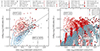 |
Fig. 1. Diagnostic diagram showing the [OIII]λ4363/Hγ vs [OIII]λ5007/[OII]λ3727 line ratios. [OII]λ3727 is the sum of the doublet [OII]λλ3726, 3728. Left panel: Plot of all the observational samples described in Sects. 2.1 and 2.2. Red is for AGN, blue for low-z SFGs, and grey for high-z sources not classified as AGN (see legend for shapes). The red and blue contours show the distribution at SDSS AGN and SFGs, respectively, including the 90%, 70%, 30%, and 10% of the populations. Right panel: Same plot, but showing the AGN and SFG models computed by Gutkin et al. (2016), Feltre et al. (2016), and Nakajima & Maiolino (2022), as described in Sect. 2.3. The tracks of the AGN and SFG models according to log U and Z are shown in Fig. B.1. The black dashed line indicates the demarcation defined in Sect. 3.4. The distribution of models and of observational samples both suggest that the dominant ionizing source in galaxies above the demarcation line is AGN. The error bars reported in the lower right corner represent the median errors of the low-redshift (left) and high-redshift (right) samples. The effect of dust attenuation on this diagnostic moves sources towards the right, without contaminating the AGN-only region with SFGs. |
High-z sources are generally distributed in the upper part of the diagnostic with respect to the local samples. We note that a non-negligible fraction of high-z sources not classified as AGN lie in the region of the diagnostic populated by local AGN, while there are also different high-z AGN falling in the same region covered by local analogues.
In the right panel we show the distribution of the photoionization models presented in Sect. 2.3 according to the same line ratios. We see here that the SFG models are predicted to occupy a limited region of this diagram, whose upper boundary almost perfectly corresponds with the distribution of SDSS SFG and local analogues, while AGN are expected to cover both the region occupied by SFGs and also the part of the diagnostic covered by the local AGN samples. Therefore, SFG models are not able to reach the part of the diagram occupied by local AGN, as expected also from the distribution of the observational samples. The opposite is not true, since AGN can occupy the region populated by SFGs, as observed for some local and high-z AGN. These considerations remain true even considering the full grid of SFG models computed in Feltre et al. (2016), as shown in Fig. C.1.
As we discuss below, to a first approximation, the ratio [OIII]λ5007/[OII]λ3727 traces the ionization parameter. At a given [OIII]λ5007/[OII]λ3727, AGN photoionization can reach much higher values of [OIII]λ4363/Hγ than photoionization from hot stars, which is likely a consequence, on average, of the much higher energy of ionizing photons produced by AGN; therefore, at a given ionization parameter, AGN can heat the gas much more effectively than hot stars.
It is worth noting the position of some high-z sources in this diagnostic. The AGN reported in Kokorev et al. (2023) shows an extremely strong [OIII]λ4363 line and it is placed in a region that is not covered by any model, which probably suggests a very high electron temperature and log U, as also pointed out in Kokorev et al. (2023). Another significant high-z AGN falling in the AGN-dominated region of this diagnostic is the source corresponding to the BLR centroid in the dual source described in Übler et al. (2024), where, in the IFS map, the peak of the broad-line emission spatially corresponds to the peak of the [OIII]λ4363 line emission. The other component, the [OIII]λ5007 centroid, showing a fainter [OIII]λ4363 line emission, is close to the border between the local analogues and the local AGN distribution, together with most of the high-z BLAGN. The AGN region is populated by different AGN selected among the CEERS and JADES MR JWST/NIRSpec spectra, but we also have different sources not selected as AGN, but falling in the AGN-dominated region, as pointed out above. We demonstrate in Sect. 4 that, from the stack of their spectra, we have an indication that some of these sources may host a BLAGN as well.
An interesting source in this diagnostic is the SFG reported in Topping et al. (2024). The source shows both strong [OIII]λ4363/Hγ and [OIII]λ5007/[OII]λ3727 emission line ratios, following the extrapolation of the distribution of the local analogues, but at very high values of the ionization parameters and at low metallicities (see Fig. B.1), as is indeed found by the analysis performed in Topping et al. (2024). Looking at the photoionization models, we see that the region is not covered by the models of Gutkin et al. (2016) and Feltre et al. (2016) (not even taking the whole parameter grid), but is instead covered by some AGN models according to Nakajima & Maiolino (2022), suggesting that the main source of ionizing radiation in this extreme galaxy is ambiguous.
It is worth noting that the effect of dust reddening on the line ratio [OIII]λ5007/[OII]λ3727, whose components can undergo a different amount of attenuation due to their distance in wavelengths, would move data points towards the right. This can potentially shift AGN into the SFG+AGN region under significant reddening, but not the opposite (i.e. galaxies dominated by star formation would not contaminate the AGN-only region).
3.2. [OIII]λ4363 /Hγ versus [Ne III]λ 3869 / [OII]λ3727
The diagnostic presented in Fig. 2 is based on the ratio between the [OIII]λ4363/Hγ compared to [Ne III]λ3869/[OII]λ3727. Not surprisingly, the distribution of the local and high-z sources in this diagnostic is very similar to that described in the previous diagnostic. The [Ne III]λ3869/[OII]λ3727 ratio correlates closely with [OIII]λ5007/[OII]λ3727 in AGN and in SFGs, as shown by Witstok et al. (2021), and as expected given that neon and oxygen are both α-elements and given that Ne+ and O+ have similar ionization potentials. The disadvantage of [Ne III]λ3869 relative to [OIII]λ5007 is that it is typically much fainter. The advantage of [Ne III]λ3869 is that it is at a shorter wavelength, and hence observable at higher redshift (out to z ∼ 12.3 with NIRSpec), and is closer in wavelength to [OII]λ3727, and hence the [Ne III]λ3869/[OII]λ3727 ratio is much less affected by dust reddening. As in the previous diagram, normal SFGs and local analogues are distributed in the lower right of the diagram, in the same region covered by SFG models, while AGN can be distributed over a wider area, including the upper left part, which cannot be reached by any SFG models or samples. As for the diagnostic described in Sect. 3.1, the separation between the two populations holds, even considering the whole grid of the parameter space of the Gutkin et al. (2016) SFG models, as presented in Fig. C.1.
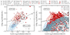 |
Fig. 2. Same as Fig. 1, but for the line ratios [OIII]λ4363/Hγ vs [Ne III]λ3869/[OII]λ3727. Based on the distribution of observational samples and models, this diagnostic diagram also identifies a region that can be populated only by AGN. |
Even if the local analogues are less numerous than in Fig. 1 (simply because there are fewer reported [Ne III]λ3869 fluxes in the literature), their distributions again seem to be an extrapolation of the distribution of local SFGs towards higher log U and lower metallicities (see Fig. B.1). The sources that were clearly in the AGN region in the previous diagnostic are still above the SFG distribution in this diagram, and the sources not identified as AGN but lying in the AGN region of the diagnostic in Fig. 1 are in the same region in Fig. 2. In addition to this latter sample, in Fig. 2 there are a few other sources from the CEERS and JADES samples that were not in the diagnostic of Fig. 1 because the [OIII]λ5007 line was not available, due to the presence of a detector gap. The AGN region is also populated by three additional sources reported in Nakajima et al. (2023) and not classified as AGN in the literature. Their location, however, is still close to the border of the SFG distribution.
The diagnostic diagram presented in this section has some similarity with the OHNO diagram that involves the [OIII]λ5007/Hβ versus [Ne III]λ3869/[OII]λ3727 line ratios (Backhaus et al. 2022, 2023; Zeimann et al. 2015; Cleri et al. 2023; Trump et al. 2023; Feuillet et al. 2024; Killi et al. 2024). The latter is mainly an ionization-sensitive diagram (ionization parameter, shape of the ionizing continuum), but it is also sensitive to metallicity and at high redshift can be affected by low-metallicity galaxy contamination (Scholtz et al. 2023). Instead, the O3Hg versus Ne3O2 diagnostic is more stable, also at high redshift, as the separation between the AGN and SFG populations is principally based on a different gas temperature, as we discuss further in Sect. 4.
3.3. [OIII]λ4363 /Hγ versus [OIII]λ5007 /[OIII]λ4363
The third diagnostic is presented in Fig. 3 and is based on the ratio of [OIII]λ4363/Hγ to [OIII]λ5007/[OIII]λ4363. This diagnostic was also reported in Übler et al. (2024). Looking at the distribution of SDSS SFGs and AGN in the left panel, we note that there is more overlap between the two populations with respect to the previous diagnostics, but there is still a region, characterized by high values of [OIII]λ4363/Hγ and high [OIII]λ5007/[OIII]λ4363, that is populated only by local AGN. The distribution of local analogues seems again to be an extrapolation of the trend of the SDSS SFG distribution. In this diagram there are very few high-z galaxies that are in the AGN-only region of the diagnostic, while most of them are shifted towards lower values of [OIII]λ5007/[OIII]λ4363, even in a region that is not covered by the current photoionization models, as is evident in the right panel. This trend is emblematically represented by the two extreme AGN reported in Kokorev et al. (2023) and in Furtak et al. (2023). Given the strength of their [OIII]λ4363 line emission, they are placed in the upper left part of the plot in a region that cannot be reproduced by any model. The same trend is shown by most of the galaxies that were not selected as AGN, but that lie in the AGN region of the two diagnostics presented above. The distribution of the SFG models matches the distribution of the local galaxies, in particular in its boundary with the AGN-only region, while AGN models cover both the region occupied by SFGs and the region populated only by AGN samples.
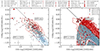 |
Fig. 3. Same as Fig. 1, but for the line ratios [OIII]λ4363/Hγ vs [OIII]λ5007 /[OIII]λ4363. In the left panel the arrow on the AGN reported in Furtak et al. (2023) is for visualization purposes only since it would be located at O33∼0. The cut in SFG models described in Sect. 2.3 allowed us to identify an AGN-only region of the diagnostic to the right of the black dashed line. |
In this diagram, assuming the whole grid of parameters of the Feltre et al. (2016) models, we would have a complete overlap between the SFG and AGN models (see Fig. C.1). However, the upper left part of the diagnostic would be covered by SFG models characterized by high values of log U and high metallicities, a condition not observed in any of our galaxy samples (see Appendix A) nor in general in the literature (Kaasinen et al. 2018; Ji & Yan 2022; Grasha et al. 2022).
3.4. Defining the locus of AGN-only objects
For the three diagnostic diagrams described above, we were able to trace clear demarcation lines providing a separation between the AGN-dominated regions and the regions where SFGs and AGN can overlap. To do so, we considered both the photoionization models and the observational sample distributions. The demarcation lines for the O3Hg versus O32 diagnostic diagram are defined as follows:
 (3)
(3)
 (4)
(4)
Similarly, for the O3Hg versus Ne3O2 diagnostic diagram, the demarcation lines are
 (5)
(5)
 (6)
(6)
Finally, the demarcation line for the O3Hg versus O33 diagnostic diagram is the following:
 (7)
(7)
These demarcation lines ensure that the fraction of contaminating SDSS SFGs in the AGN part of the diagnostics is less than 1–2%, while none of the local analogues lie in the AGN-only part of the three diagnostics.
Such a tiny fraction of contaminants can probably be associated with sources that are not identified as AGN by the BPT diagram (used to distinguish between SDSS SFG and AGN in this work), but that host active SMBHs. The presence of AGN contaminants among BPT-selected SFG and local analogues has already been demonstrated by recent works (Svoboda et al. 2019; Harish et al. 2023).
Furthermore, it is important to note that the AGN selection based on these demarcation lines is not a necessary condition for a source to be an AGN, but rather a sufficient condition. Objects above the demarcation line are AGN-dominated with high confidence, while objects below the demarcation line can either be SFGs or AGN.
4. Discussion
By comparing the distribution of the observational samples with the distribution of the photoionization models, we can explain why these diagnostic diagrams can separate part of the AGN population from SFGs. In Fig B.1 we plot the AGN and SFG models in the same diagnostic diagrams presented in Sect. 3, but highlighting the variation of log U and Z (i.e. the two main parameters affecting the distribution of the models in these plots). Since they are very local, we know that the SDSS AGN and SFG samples are populated mostly by solar metallicity and moderate- to low-ionization parameter sources, as shown also by the models occupying the same region of these samples in Fig. B.1. On the contrary, local analogues are characterized, on average, by lower metallicities and higher ionization parameters (such as high-z galaxies). In Figs. 1 and 2 they fill the regions that extend from the SDSS SFG towards higher [OIII]λ4363/Hγ and higher [OIII]λ5007/[OII]λ3727 or [Ne III]λ3869/ [OII]λ3727, in close agreement with the trend of photoionization models for higher log U and lower Z in the same diagnostics (see Fig. B.1).
The reason for the presence, in particular in Figs. 1 and 2, of a region that is populated only by AGN, at high [OIII]λ4363/Hγ values, can be explained in the following way. Since the [OIII]λ4363 line is a collisionally excited line generated by high energy levels, its intensity relative to Hγ is directly related to the temperature and, secondly, to the metallicity of the ISM and the ionization parameter. The main difference between the AGN and SFGs is the SED of the incident ionizing radiation. For AGN the ionizing radiation is given by the emission of the accretion disc, while for SFGs it originates from young star clusters. The former are characterized by a harder spectrum, and therefore, on average, photons that are more energetic (see Fig. 1 in Feltre et al. 2016). Higher energy per ionizing photon, deposited into the ISM, results in higher effective heating, and in turn higher electron temperature (hence higher [OIII]λ4363) at a given ionization parameter.
4.1. Stacking of the AGN candidates
To further demonstrate the effectiveness of the diagnostic diagrams proposed in this work, we explored potential tracers of AGN activity in those high-z galaxies lying in the AGN region of the diagnostics diagrams in Figs. 1 and 2, but not previously identified as AGN based on the selection performed in Scholtz et al. (2023) and Mazzolari et al. (in prep.). Our stacking procedure was as follows. We first shifted the spectra to the rest frame and normalized them to the peak of the Hα line, which was available for all the sources involved. This ensured that the bright sources were not dominating the final stacks. We then resampled each of the spectra to a common wavelength grid. We verified that the wavelength grid did not impact our conclusions by repeating the analysis using wavelength bins ranging from the best resolution (∼100 km/s) to the worst (∼150km/s). Finally, before stacking the spectra, we fitted and subtracted the continuum from the rest-frame rebinned spectra. We performed an inverse variance stacking of 15 sources (11 from CEERS and 4 from JADES).
We first fitted simultaneously the Hα and [N II] wavelength region using only a single Gaussian profile per emission line, with common full width at half maximum (FWHM) and redshift for all three emission lines. We fixed the [N II] doublet ratio to be 3. We show the narrow emission line fit in the top left panel of Fig. 4. We detected broad residuals around the Hα emission line. These broad components can arise from either a broad-line region or an outflow.
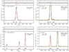 |
Fig. 4. Different fits of the spectrum derived from the stack of the sources not identified as AGN in the literature, but lying in the AGN region of the diagnostic diagrams presented in Sect. 3. The stacked spectrum in these plots is resampled at the best resolution among those of the single spectra involved (i.e. ∼100km/s), but the results do not change considering the worst resolution (i.e. ∼150km/s). Top panels: Fit of the Hα and [N II] complex with only a narrow component (left) and adding a broad component to the Hα line (right). The global fit is presented in red, while the narrow and broad Hα components are in green and yellow, respectively. In the upper panel are shown the residuals of the fit compared with the distribution of the 1σ (blue) and 3σ (red) errors on the fluxes. In the upper right part of the plots are reported the FWHM and the velocity offset of the different components considered in the fits. Lower panels: Same as above, but for the Hβ and [O III] λλ4959, 5007 doublet complex. In particular, on the right, we added to the fit of the [OIII]λ5007 a broad component with the same FWHM and velocity offset as the broad component of the Hα, but here it is not required by the fit. |
To model the broad wing in the Hα, we refitted the Hα and [N II] with two additional models, the BLR model (by fitting one additional broad Gaussian component to Hα only) and an outflow model (by adding broad Gaussian components to both Hα and [N II] with fixed FWHM and centroid). Using the Bayesian information criterion (BIC) parameter (Liddle 2007), we found that the BLR model is strongly preferred to the narrow-only fit (ΔBIC = BICHαNL − BICHαBL = 90). The broad component has a S/N of 10, making this a solid detection. On the contrary, the fit with the outflow model did not return any broad component in the [N II] lines.
We then used the same approach with the Hβ and [O III] λλ4959, 5007 complex, to test the possibility that this broad component could be associated with an outflow on larger scales, determining a broad [OIII]λ5007. In the fit shown in the last panel of Fig. 4, we imposed the broad component of the [O III] λλ4959, 5007 to have the same kinematics as the broad component of the Hα(i.e. the same FWHM and velocity offset). However, we did not find a significant broad line detection, and therefore outflow, in the [O III] λλ4959, 5007. In particular, by imposing a broad outflow component to the [O III] λλ4959, 5007 and comparing it with the NL-only fit, it gives a ![Mathematical equation: $ \Delta \mathrm{BIC}= \mathrm{BIC}_{[\rm OIII]\ \mathrm{NL}} - \mathrm{BIC}_{[\rm OIII]\ \mathrm{BL}}= 4 $](/articles/aa/full_html/2024/11/aa50407-24/aa50407-24-eq9.gif) , meaning that the two models are almost equally preferred, and hence a broad [OIII]λ5007 component is not required.
, meaning that the two models are almost equally preferred, and hence a broad [OIII]λ5007 component is not required.
The absence of a counterpart in (brighter) [OIII]λ5007 strongly disfavours an outflow origin of the broad component of Hα. Therefore, the detection of a broad component in the Hα emission line suggests the presence of an AGN BLR in the spectra of at least some of these galaxies, which is too weak to be detected in the individual spectra. This indicates that galaxies located in the upper region of our diagnostic diagrams, even if originally not classified as AGN, actually may host faint Type I AGN. This result provides confidence that the diagnostic diagrams presented in this work are effective in identifying AGN above our proposed demarcation lines, although they cannot distinguish between AGN and SFGs below the demarcation line.
4.2. Ruling out [FeII]λ4360 contamination
We investigate the possibility that the [OIII]λ4363 emission line in the high-z sources located in the AGN-only region of the diagnostics could be contaminated by the [FeII]λ4360 emission line (Curti et al. 2017; Arellano-Córdova et al. 2022). Most of the high-z [OIII]λ4363 detections come from JWST MR spectra, whose resolution is not high enough to disentangle the two lines. Curti et al. (2017) showed that this contamination is possible, but most likely in high-metallicity galaxies, while our high-z sample is generally metal poor.
To investigate the possible iron contamination of the [OIII]λ4363 line, we consider the close [FeII]λ4288 emission line, which is isolated and originates from the same energy level as the [FeII]λ4360. We ran a grid of Cloudy photoionization models over a wide range of metallicities (with  ) and ionization parameters (with
  ), and found that the flux ratio of [FeII]λ4288/[FeII]λ43602 is roughly a constant of ∼1.25. Therefore, we can use the [FeII]λ4288 emission line to reliably constrain the intensity of the [FeII]λ4360. We did not detect the [FeII]λ4288 line in any of the high-z sources in the AGN-only regions of the diagnostics. Even when we performed a weighted spectral stacking of all the spectra in the same region, the [FeII]λ4288 emission line remained undetected. Therefore, we conclude that any possible contribution to the [OIII]λ4363 detections given by the [FeII]λ4360 emission line is negligible.
4.3. Impact on metallicity estimates and strong-line metallicity diagnostics
The [OIII]λ4363 emission line has been widely used in the literature to derive metallicities via the Te-method (see Maiolino & Mannucci 2019, for a review), although Marconi et al. (2024) have shown that these metallicities may be biased low. The metallicities inferred from the Te-method have then been used to calibrate the strong-line metallicity diagnostics (i.e. ratios of optical emission lines typically much stronger than the auroral lines, which can be used to estimate the metallicities on larger samples of galaxies). These calibrations have been inferred both by using local samples of galaxies (e.g. Maiolino et al. 2008; Bian et al. 2018; Curti et al. 2020) and, especially with JWST, at high redshift (Sanders et al. 2023; Laseter et al. 2024).
In most of these past studies care was taken to only use SFGs, or to assume that the gas ionization was dominated by young hot stars. The finding of consistent populations of AGN at high redshift by recent JWST studies, and especially our own finding in this paper that a significant number of strong [OIII]λ4363 detections at high redshift are due to AGN heating, may appear concerning when using this transition to infer the gas metallicity. However, the [OIII]λ4363 line (together with [OIII]λ5007, or [Ne III]λ3869 as a proxy when the other is not available) provides a measurement of the temperature in the O+2 zone, regardless of the nature of the ionizing source. So its reliability remains unaffected in the case of photoionization by AGN (modulo the potential biases discussed in Marconi et al. 2024, which are an issue, also for SFGs). What is important is to properly use this information to infer the metallicity, and in particular by applying the proper ionization correction factors, which are different in the case of AGN and SFGs. In particular, once the abundance of O+2/H+ is derived, one has to estimate the contribution to the abundances from O+3/H+ and O+/H+. The former is very difficult to assess, even in AGN, as there are no [OIV] strong transitions in the wavelength ranges typically accessible. Dors et al. (2020) estimate that, even in AGN, the contribution of O+3/H+ is typically negligible. The contribution from O+/H+ is estimated from the [OII]λ3727 doublet; however, the key issue is that the temperature of the O+ region is different from the temperature of the O+2 region probed by the [OIII]λ4363 line. If [OII] auroral lines are not available (as in the vast majority of the cases at high redshift), then one has to assume a relation between T(O+) and T(O+2). This relation has been extensively explored in local SFGs; however, it cannot be applied to AGN. Assuming in AGN the same temperature relation as for SFGs results in a large underestimation of the metallicities (Dors et al. 2015). This issue is greatly mitigated once AGN-bespoke relations between T(O+) and T(O+2) are adopted (Dors et al. 2020).
In summary, the fact that at high redshift [OIII]λ4363 is boosted by AGN heating does not prevent it from being used to measure the metallicity in those galaxies, provided that the proper ionization correction factors are adopted and, in particular, the adequate T(O+) and T(O+2) is adopted (in absence of [OII] auroral lines).
However, the presence of AGN ionization, excitation, and heating certainly affects the empirical calibrations of the strong line diagnostics. At a given gas temperature the AGN radiation (with different ionizing shape and, typically, higher ionization parameter) results in a different ionization structure of the gas clouds, and also different collisional excitation rates of the various transitions typically used in the strong line diagnostics ([OIII], [OII], [NeIII], [NII], [SII]). As a consequence, separate and different empirical metallicity calibrations should be inferred for SFGs and AGN host galaxies. This has been attempted in the local universe (Dors 2021). However, the same effort should be undertaken at high redshift, given the large abundance of AGN. Inferring empirical strong-line metallicity calibrations differentiating AGN and SFGs will be the focus of a separate dedicated paper.
5. Conclusions
While JWST has revealed that some of the classical AGN diagnostics break down at high redshift, it has also opened the opportunity to explore new diagnostics. In this work we studied the possibility of selecting AGN using the [OIII]λ4363 auroral line, whose detection in large numbers of high-z galaxies has become possible with JWST. In particular, we proposed three new diagnostic diagrams, and three corresponding demarcation lines, that allow a large population of AGN to be identified from SFGs by providing a sufficient (but not necessary) condition to claim the presence of an AGN.
To demonstrate the effectiveness of these diagnostics, we used multiple observational samples of local and high-z SFGs and AGN as well as photoionization models from Feltre et al. (2016) and Nakajima & Maiolino (2022). We specifically proposed the following three diagnostic diagrams:
-
[OIII]λ4363/Hγ versus [OIII]5007/[OII]3727. This is the most thoroughly explored diagram from the empirical perspective (it has the largest observational test sample), and can be used with NIRSpec out to z < 9.4;
-
[OIII]λ4363/Hγ versus [NeIII]3869/[OII]3727. This diagram is the least sensitive to dust extinction given the wavelength proximity of both line ratios. Additionally, it can be used with NIRSpec out to z < 10.9;
-
[OIII]λ4363/Hγ versus [OIII]5007/[OIII]λ4363. Among the three, this is the one with the smallest region where AGN can be safely identified, but it is also relatively dust insensitive and requires the detection of only three lines instead of four, making it applicable to larger samples.
In each of these cases we provided a demarcation line above which (i.e. with higher [OIII]λ4363/Hγ values) objects can be safely identified as hosting an AGN that dominates the nebular emission lines excitation.
We illustrated that at least some of the few objects falling into the AGN-only region and not previously identified as AGN actually show AGN signatures when stacked. This further supports the effectiveness of the diagnostics. At the same time, we did not find any indication of [FeII]λ4360 contamination of the [OIII]λ4363 emission line in these sources, which could in principle artificially increase the [OIII]λ4363 line due to blending effects.
The physics behind these diagnostics is tightly linked to the primary property of AGN (i.e. the hardness of the ionizing spectrum). The average energy of the AGN’s ionizing photons is much higher than the energy of hot young stars in SFGs. Therefore, at a given ionizing radiation field intensity, AGN photons are more effective in heating the ionized gas than those in SF regions, hence yielding higher temperature, and hence higher [OIII]λ4363 relative to Hγ (which accounts for the overall photoionizing radiation field).
We note that being above the demarcation line in the proposed diagrams is a sufficient but not necessary condition for an object to be identified as an AGN. Galaxies located below the demarcation lines can be powered by star formation and/or AGN. At the same time, the contamination from SFG is almost completely negligible in the upper part of the diagnostics, as demonstrated by the distribution of low-redshift observational samples and photoionization models. Moreover, the few high-redshift ambigous cases in the AGN-only region also turn out to be AGN based on the stacking.
Finally, we note that the fact that strong auroral lines are often associated with AGN does not imply that they cannot be used for direct metallicity measurements (provided that proper ionization corrections are applied), but it does affect the calibration of strong line metallicity diagnostics, calling for new AGN-specific calibrations of these diagrams.
The boundary is determined by the common outer envelopes of SDSS SFGs and local analogues as these two samples differ significantly in number and occupy different regions in the parameter space.
Our calculation takes into account six lines from Fe+ blended at 4288 Å and eight lines from Fe+ blended at 4360 Å, although most of the fluxes are contributed by [FeII]λ4287.39 and [FeII]λ4359.33.
Acknowledgments
We thank the anonymous referee for useful suggestions which improved the quality of the paper. GM acknowledges useful conversations with Roberto Gilli, Marcella Brusa, Sandro Tacchella, William Baker, Callum Witten, Bartolomeo Trefoloni, Lola Danhaive, Ignas Juodzbalis, Amanda Stoffer, Brian Xing Jiang, and William McClaymont. FDE, JS and RM acknowledge support by the Science and Technology Facilities Council (STFC), from the ERC Advanced Grant 695671 “QUENCH”, and by the UKRI Frontier Research grant RISEandFALL. RM also acknowledges funding from a research professorship from the Royal Society. HÜ gratefully acknowledges support by the Isaac Newton Trust and by the Kavli Foundation through a Newton-Kavli Junior Fellowship.
References
- Abazajian, K. N., Adelman-McCarthy, J. K., Agüeros, M. A., et al. 2009, ApJS, 182, 543 [Google Scholar]
- Amorín, R., Pérez-Montero, E., Contini, T., et al. 2015, A&A, 578, A105 [NASA ADS] [CrossRef] [EDP Sciences] [Google Scholar]
- Arellano-Córdova, K. Z., Berg, D. A., Chisholm, J., et al. 2022, ApJ, 940, L23 [CrossRef] [Google Scholar]
- Armah, M., Dors, O. L., Aydar, C. P., et al. 2021, MNRAS, 508, 371 [NASA ADS] [CrossRef] [Google Scholar]
- Backhaus, B. E., Trump, J. R., Cleri, N. J., et al. 2022, ApJ, 926, 161 [NASA ADS] [CrossRef] [Google Scholar]
- Backhaus, B. E., Bridge, J. S., Trump, J. R., et al. 2023, ApJ, 943, 37 [NASA ADS] [CrossRef] [Google Scholar]
- Baldwin, J. A., Phillips, M. M., & Terlevich, R. 1981, PASP, 93, 5 [Google Scholar]
- Berg, D. A., Skillman, E. D., Marble, A. R., et al. 2012, ApJ, 754, 98 [NASA ADS] [CrossRef] [Google Scholar]
- Bian, F., Kewley, L. J., & Dopita, M. A. 2018, ApJ, 859, 175 [CrossRef] [Google Scholar]
- Blanc, G. A., Kewley, L., Vogt, F. P. A., & Dopita, M. A. 2015, ApJ, 798, 99 [Google Scholar]
- Bogdán, Á., Goulding, A. D., Natarajan, P., et al. 2023, Nat. Astron., submitted [arXiv:2305.15458] [Google Scholar]
- Brinchmann, J. 2023, MNRAS, 525, 2087 [NASA ADS] [CrossRef] [Google Scholar]
- Bunker, A. J., Cameron, A. J., Curtis-Lake, E., et al. 2024, A&A, 690, A288 [NASA ADS] [CrossRef] [EDP Sciences] [Google Scholar]
- Calabro, A., Castellano, M., Zavala, J. A., et al. 2024, ArXiv e-prints [arXiv:2403.12683] [Google Scholar]
- Calzetti, D., Armus, L., Bohlin, R. C., et al. 2000, ApJ, 533, 682 [NASA ADS] [CrossRef] [Google Scholar]
- Carton, D., Brinchmann, J., Shirazi, M., et al. 2017, MNRAS, 468, 2140 [NASA ADS] [CrossRef] [Google Scholar]
- Chisholm, J., Berg, D. A., Endsley, R., et al. 2024, MNRAS, submitted [arXiv:2402.18643] [Google Scholar]
- Cleri, N. J., Olivier, G. M., Hutchison, T. A., et al. 2023, ApJ, 953, 10 [NASA ADS] [CrossRef] [Google Scholar]
- Curti, M., Cresci, G., Mannucci, F., et al. 2017, MNRAS, 465, 1384 [Google Scholar]
- Curti, M., Maiolino, R., Cirasuolo, M., et al. 2020, MNRAS, 492, 821 [CrossRef] [Google Scholar]
- Curti, M., D’Eugenio, F., Carniani, S., et al. 2023, MNRAS, 518, 425 [Google Scholar]
- Curti, M., Maiolino, R., Curtis-Lake, E., et al. 2024, A&A, 684, A75 [NASA ADS] [CrossRef] [EDP Sciences] [Google Scholar]
- Curtis-Lake, E., Carniani, S., Cameron, A., et al. 2022, ArXiv e-prints [arXiv:2212.04568] [Google Scholar]
- Dopita, M. A., Fischera, J., Sutherland, R. S., et al. 2006, ApJS, 167, 177 [NASA ADS] [CrossRef] [Google Scholar]
- Dopita, M. A., Shastri, P., Davies, R., et al. 2015, ApJS, 217, 12 [NASA ADS] [CrossRef] [Google Scholar]
- Dors, O. L. 2021, MNRAS, 507, 466 [NASA ADS] [CrossRef] [Google Scholar]
- Dors, O. L., Cardaci, M. V., Hägele, G. F., et al. 2015, MNRAS, 453, 4102 [Google Scholar]
- Dors, O. L., Maiolino, R., Cardaci, M. V., et al. 2020, MNRAS, 496, 3209 [NASA ADS] [CrossRef] [Google Scholar]
- Eldridge, J. J., Stanway, E. R., Xiao, L., et al. 2017, PASA, 34, e058 [Google Scholar]
- Feltre, A., Charlot, S., & Gutkin, J. 2016, MNRAS, 456, 3354 [Google Scholar]
- Ferland, G. J., Porter, R. L., van Hoof, P. A. M., et al. 2013, Rev. Mex. Astron. Astrofis., 49, 137 [Google Scholar]
- Ferruit, P., Jakobsen, P., Giardino, G., et al. 2022, A&A, 661, A81 [NASA ADS] [CrossRef] [EDP Sciences] [Google Scholar]
- Feuillet, L. M., Meléndez, M., Kraemer, S., et al. 2024, ApJ, 962, 104 [NASA ADS] [CrossRef] [Google Scholar]
- Finkelstein, S. L., Bagley, M. B., Arrabal Haro, P., et al. 2022, ApJ, 940, L55 [NASA ADS] [CrossRef] [Google Scholar]
- Furtak, L. J., Labbé, I., Zitrin, A., et al. 2023, ArXiv e-prints [arXiv:2308.05735] [Google Scholar]
- Gardner, J. P., Mather, J. C., Abbott, R., et al. 2023, PASP, 135, 068001 [NASA ADS] [CrossRef] [Google Scholar]
- Giallongo, E., Grazian, A., Fiore, F., et al. 2019, ApJ, 884, 19 [Google Scholar]
- Gilli, R., Norman, C., Calura, F., et al. 2022, A&A, 666, A17 [NASA ADS] [CrossRef] [EDP Sciences] [Google Scholar]
- Goulding, A. D., Greene, J. E., Setton, D. J., et al. 2023, ApJ, 955, L24 [NASA ADS] [CrossRef] [Google Scholar]
- Grasha, K., Chen, Q. H., Battisti, A. J., et al. 2022, ApJ, 929, 118 [NASA ADS] [CrossRef] [Google Scholar]
- Greene, J. E., Labbe, I., Goulding, A. D., et al. 2023, ApJ, submitted [arXiv:2309.05714] [Google Scholar]
- Groves, B. A., Heckman, T. M., & Kauffmann, G. 2006, MNRAS, 371, 1559 [NASA ADS] [CrossRef] [Google Scholar]
- Gutkin, J., Charlot, S., & Bruzual, G. 2016, MNRAS, 462, 1757 [Google Scholar]
- Harikane, Y., Zhang, Y., Nakajima, K., et al. 2023, ApJ, submitted [arXiv:2303.11946] [Google Scholar]
- Harish, S., Malhotra, S., Rhoads, J. E., et al. 2023, ApJ, 945, 157 [NASA ADS] [CrossRef] [Google Scholar]
- Hirschmann, M., Charlot, S., Feltre, A., et al. 2019, MNRAS, 487, 333 [NASA ADS] [CrossRef] [Google Scholar]
- Izotov, Y. I., Stasińska, G., Meynet, G., Guseva, N. G., & Thuan, T. X. 2006, A&A, 448, 955 [CrossRef] [EDP Sciences] [Google Scholar]
- Izotov, Y. I., Thuan, T. X., Guseva, N. G., & Liss, S. E. 2018, MNRAS, 473, 1956 [NASA ADS] [CrossRef] [Google Scholar]
- Izotov, Y. I., Guseva, N. G., Fricke, K. J., & Henkel, C. 2019, A&A, 623, A40 [NASA ADS] [CrossRef] [EDP Sciences] [Google Scholar]
- Izotov, Y. I., Guseva, N. G., Fricke, K. J., et al. 2021, A&A, 646, A138 [NASA ADS] [CrossRef] [EDP Sciences] [Google Scholar]
- Jakobsen, P., Ferruit, P., Alves de Oliveira, C., et al. 2022, A&A, 661, A80 [NASA ADS] [CrossRef] [EDP Sciences] [Google Scholar]
- Ji, X., & Yan, R. 2022, A&A, 659, A112 [NASA ADS] [CrossRef] [EDP Sciences] [Google Scholar]
- Juodžbalis, I., Ji, X., Maiolino, R., et al. 2024a, MNRAS, submitted [arXiv:2407.08643] [Google Scholar]
- Juodžbalis, I., Maiolino, R., Baker, W. M., et al. 2024b, ArXiv e-prints [arXiv:2403.03872] [Google Scholar]
- Kaasinen, M., Kewley, L., Bian, F., et al. 2018, MNRAS, 477, 5568 [NASA ADS] [CrossRef] [Google Scholar]
- Kewley, L. J., Dopita, M. A., Sutherland, R. S., Heisler, C. A., & Trevena, J. 2001, ApJ, 556, 121 [Google Scholar]
- Killi, M., Watson, D., Brammer, G., et al. 2024, A&A, 691, A52 [NASA ADS] [CrossRef] [EDP Sciences] [Google Scholar]
- Kocevski, D. D., Onoue, M., Inayoshi, K., et al. 2023, ArXiv e-prints [arXiv:2302.00012] [Google Scholar]
- Kokorev, V., Fujimoto, S., Labbe, I., et al. 2023, ApJ, 957, L7 [NASA ADS] [CrossRef] [Google Scholar]
- Kovacs, O. E., Bogdan, A., Natarajan, P., et al. 2024, ArXiv e-prints [arXiv:2403.14745] [Google Scholar]
- Kriek, M., Shapley, A. E., Reddy, N. A., et al. 2015, ApJS, 218, 15 [NASA ADS] [CrossRef] [Google Scholar]
- Labbe, I., Bezanson, R., Atek, H., et al. 2021, UNCOVER: Ultra-deep NIRCam and NIRSpec Observations Before the Epoch of Reionization, JWST Proposal. Cycle, 1, 2561 [Google Scholar]
- Laseter, I. H., Maseda, M. V., Curti, M., et al. 2024, A&A, 681, A70 [NASA ADS] [CrossRef] [EDP Sciences] [Google Scholar]
- Liddle, A. R. 2007, MNRAS, 377, L74 [NASA ADS] [Google Scholar]
- Lilly, S. J., Le Fèvre, O., Renzini, A., et al. 2007, ApJS, 172, 70 [Google Scholar]
- Luo, B., Brandt, W. N., Xue, Y. Q., et al. 2017, ApJS, 228, 2 [Google Scholar]
- Maiolino, R., & Mannucci, F. 2019, A&ARv, 27, 3 [Google Scholar]
- Maiolino, R., Nagao, T., Grazian, A., et al. 2008, A&A, 488, 463 [NASA ADS] [CrossRef] [EDP Sciences] [Google Scholar]
- Maiolino, R., Risaliti, G., Signorini, M., et al. 2024a, MNRAS, submitted [arXiv:2405.00504] [Google Scholar]
- Maiolino, R., Scholtz, J., Witstok, J., et al. 2024b, Nature, 627, 59 [NASA ADS] [CrossRef] [Google Scholar]
- Maiolino, R., Scholtz, J., Curtis-Lake, E., et al. 2024c, A&A, 691, A145 [NASA ADS] [CrossRef] [EDP Sciences] [Google Scholar]
- Maiolino, R., Uebler, H., Perna, M., et al. 2024d, A&A, 687, A67 [NASA ADS] [CrossRef] [EDP Sciences] [Google Scholar]
- Marconi, A., Amiri, A., Feltre, A., et al. 2024, A&A, 689, A78 [NASA ADS] [CrossRef] [EDP Sciences] [Google Scholar]
- Matthee, J., Naidu, R. P., Brammer, G., et al. 2023, ArXiv e-prints [arXiv:2306.05448] [Google Scholar]
- Mignoli, M., Feltre, A., Bongiorno, A., et al. 2019, A&A, 626, A9 [NASA ADS] [CrossRef] [EDP Sciences] [Google Scholar]
- Mingozzi, M., Belfiore, F., Cresci, G., et al. 2020, A&A, 636, A42 [NASA ADS] [CrossRef] [EDP Sciences] [Google Scholar]
- Nakajima, K., & Maiolino, R. 2022, MNRAS, 513, 5134 [NASA ADS] [CrossRef] [Google Scholar]
- Nakajima, K., Ouchi, M., Xu, Y., et al. 2022, ApJS, 262, 3 [CrossRef] [Google Scholar]
- Nakajima, K., Ouchi, M., Isobe, Y., et al. 2023, ArXiv e-prints [arXiv:2301.12825] [Google Scholar]
- Nandra, K., Laird, E. S., Aird, J. A., et al. 2015, ApJS, 220, 10 [NASA ADS] [CrossRef] [Google Scholar]
- Perna, M., Lanzuisi, G., Brusa, M., Cresci, G., & Mignoli, M. 2017, A&A, 606, A96 [NASA ADS] [CrossRef] [EDP Sciences] [Google Scholar]
- Pontoppidan, K. M., Barrientes, J., Blome, C., et al. 2022, ApJ, 936, L14 [NASA ADS] [CrossRef] [Google Scholar]
- Pustilnik, S. A., Kniazev, A. Y., Perepelitsyna, Y. A., & Egorova, E. S. 2020, MNRAS, 493, 830 [NASA ADS] [CrossRef] [Google Scholar]
- Pustilnik, S. A., Egorova, E. S., Kniazev, A. Y., et al. 2021, MNRAS, 507, 944 [NASA ADS] [CrossRef] [Google Scholar]
- Rigby, J., Perrin, M., McElwain, M., et al. 2023, PASP, 135, 048001 [NASA ADS] [CrossRef] [Google Scholar]
- Robertson, B. E., Tacchella, S., Johnson, B. D., et al. 2022, ArXiv e-prints [arXiv:2212.04480] [Google Scholar]
- Sanders, R. L., Shapley, A. E., Topping, M. W., Reddy, N. A., & Brammer, G. B. 2023, ArXiv e-prints [arXiv:2301.06696] [Google Scholar]
- Scholtz, J., Maiolino, R., D’Eugenio, F., et al. 2023, A&A submitted [arXiv:2311.18731] [Google Scholar]
- Scholtz, J., Witten, C., Laporte, N., et al. 2024, A&A, 687, A283 [NASA ADS] [CrossRef] [EDP Sciences] [Google Scholar]
- Seyfert, C. K. 1943, ApJ, 97, 28 [NASA ADS] [CrossRef] [Google Scholar]
- Simmonds, C., Bauer, F. E., Thuan, T. X., et al. 2016, A&A, 596, A64 [NASA ADS] [CrossRef] [EDP Sciences] [Google Scholar]
- Svoboda, J., Douna, V., Orlitová, I., & Ehle, M. 2019, ApJ, 880, 144 [NASA ADS] [CrossRef] [Google Scholar]
- Thomas, A. D., Dopita, M. A., Shastri, P., et al. 2017, ApJS, 232, 11 [NASA ADS] [CrossRef] [Google Scholar]
- Topping, M. W., Stark, D. P., Senchyna, P., et al. 2024, MNRAS, 529, 3301 [NASA ADS] [CrossRef] [Google Scholar]
- Treu, T., Roberts-Borsani, G., Bradac, M., et al. 2022, ApJ, 935, 110 [NASA ADS] [CrossRef] [Google Scholar]
- Trump, J. R., Arrabal Haro, P., Simons, R. C., et al. 2023, ApJ, 945, 35 [NASA ADS] [CrossRef] [Google Scholar]
- Übler, H., Maiolino, R., Curtis-Lake, E., et al. 2023, A&A, 677, A145 [NASA ADS] [CrossRef] [EDP Sciences] [Google Scholar]
- Übler, H., Maiolino, R., Pérez-González, P. G., et al. 2024, MNRAS, 531, 355 [CrossRef] [Google Scholar]
- Veilleux, S., & Osterbrock, D. E. 1987, ApJS, 63, 295 [Google Scholar]
- Vidal-García, A., Plat, A., Curtis-Lake, E., et al. 2024, MNRAS, 527, 7217 [Google Scholar]
- Vito, F., Gilli, R., Vignali, C., et al. 2016, MNRAS, 463, 348 [NASA ADS] [CrossRef] [Google Scholar]
- Vito, F., Brandt, W. N., Yang, G., et al. 2018, MNRAS, 473, 2378 [Google Scholar]
- Wang, B., de Graaff, A., Davies, R. L., et al. 2024, A&A [Google Scholar]
- Witstok, J., Smit, R., Maiolino, R., et al. 2021, MNRAS, 508, 1686 [NASA ADS] [CrossRef] [Google Scholar]
- Xue, Y. Q., Luo, B., Brandt, W. N., et al. 2016, ApJS, 224, 15 [Google Scholar]
- Yang, H., Malhotra, S., Gronke, M., et al. 2017a, ApJ, 844, 171 [NASA ADS] [CrossRef] [Google Scholar]
- Yang, H., Malhotra, S., Rhoads, J. E., & Wang, J. 2017b, ApJ, 847, 38 [NASA ADS] [CrossRef] [Google Scholar]
- Yang, G., Caputi, K. I., Papovich, C., et al. 2023, ApJ, 950, L5 [NASA ADS] [CrossRef] [Google Scholar]
- Zeimann, G. R., Ciardullo, R., Gebhardt, H., et al. 2015, ApJ, 798, 29 [Google Scholar]
Appendix A: Cut in photoionization models
In Fig. A.1 we show the distribution of the SDSS SFG and local analogues samples in the log U versus log OH plane as derived following the likelihood procedure with the Gutkin et al. (2016) models described in Sec. 2.3. Even considering different values of the C/O, ξ, and nH parameters in the models, the chosen excluded region contains less than 0.1% of the sources (located very close to the borders).
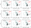 |
Fig. A.1. Distribution of the SDSS SFG sample (circles) and local analogues (triangles) in the log U vs log OH plane, according to the likelihood procedure with the Feltre et al. (2016) models described in Sect. 2.3. In each panel, we also show (red dashed line), the region of the parameter space that we decided to exclude, a posteriori, from the same photoionization models. The upper panels show the variation in the distribution of the sources by considering models with different electron densities nH. The middle panels show different dust-to-metal ratios ξ, the bottom panels different C/O abundance. The excluded region is never significantly populated by any source in all the panels. |
Appendix B: Photoionization model properties
In Fig. B.1 we show the distribution of the SFG and AGN photoionization models from Gutkin et al. (2016), Feltre et al. (2016), and Nakajima & Maiolino (2022) in the three diagnostic diagrams presented in Sec. 3. In particular, the plots highlight the variation of log U and Z of the models across the diagnostics.
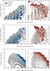 |
Fig. B.1. Distribution of the photoionization models computed in Feltre et al. (2016) (circles) and Nakajima & Maiolino (2022) (stars) with respect to the line ratios reported in Fig. 1 (top panel), Fig. 2 (central panel), and Fig. 3 (bottom panel). The photoionization models for SFG are reported on the right, while the AGN models are on the left. The points are colour-coded according to their metallicity (the stronger the colour, the higher the metallicity), and the marker size depends on the ionization parameter (the larger the marker, the higher the ionization parameter). The maximum and minimum values of Z and log U for the two classes of models are reported in the top part of the top panels. |
Appendix C: Diagnostic diagrams including all photoionization models
The demarcation lines presented in Sec. 3.4 were defined considering both the distribution of the observational samples and of photoionization models with the cut described in Sec. 2.3 and shown in Fig. A.1. If we consider the entire grid of parameters for the models of Gutkin et al. (2016) and Feltre et al. (2016), we obtain the distributions shown in Fig. C.1. In this case, the demarcation lines for the O3Hg-O32 and O3Hg-Ne3O2 diagnostic plots still hold, except for a very small fraction of SFG models populating the AGN-only part of the two diagnostics. On the contrary, in the O3Hg-O33 diagnostic plot, there is an almost complete superposition between the SFG and AGN models. Even if this superposition is determined by highly unlikely combinations of parameters in the models, we cannot completely rule out the possibility that the AGN-only region of the O3Hg-O33 diagnostic diagram could actually be partially populated also by SFG.
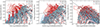 |
Fig. C.1. Same plots reported in the right panels of Fig. 1, Fig. 2 and Fig. 3 (from left to right), but showing all the models computed in Gutkin et al. (2016), Feltre et al. (2016), and Nakajima & Maiolino (2022), i.e. without the cut described in Sect. 2.3. The demarcation lines for the O3Hg-O32 and O3Hg-Ne3O2 still hold, while there is an almost complete superposition between SFG and AGN models in the O3Hg-O33 diagnostic diagram. |
All Tables
All Figures
|
Fig. 1. Diagnostic diagram showing the [OIII]λ4363/Hγ vs [OIII]λ5007/[OII]λ3727 line ratios. [OII]λ3727 is the sum of the doublet [OII]λλ3726, 3728. Left panel: Plot of all the observational samples described in Sects. 2.1 and 2.2. Red is for AGN, blue for low-z SFGs, and grey for high-z sources not classified as AGN (see legend for shapes). The red and blue contours show the distribution at SDSS AGN and SFGs, respectively, including the 90%, 70%, 30%, and 10% of the populations. Right panel: Same plot, but showing the AGN and SFG models computed by Gutkin et al. (2016), Feltre et al. (2016), and Nakajima & Maiolino (2022), as described in Sect. 2.3. The tracks of the AGN and SFG models according to log U and Z are shown in Fig. B.1. The black dashed line indicates the demarcation defined in Sect. 3.4. The distribution of models and of observational samples both suggest that the dominant ionizing source in galaxies above the demarcation line is AGN. The error bars reported in the lower right corner represent the median errors of the low-redshift (left) and high-redshift (right) samples. The effect of dust attenuation on this diagnostic moves sources towards the right, without contaminating the AGN-only region with SFGs. |
| In the text | |
|
Fig. 2. Same as Fig. 1, but for the line ratios [OIII]λ4363/Hγ vs [Ne III]λ3869/[OII]λ3727. Based on the distribution of observational samples and models, this diagnostic diagram also identifies a region that can be populated only by AGN. |
| In the text | |
|
Fig. 3. Same as Fig. 1, but for the line ratios [OIII]λ4363/Hγ vs [OIII]λ5007 /[OIII]λ4363. In the left panel the arrow on the AGN reported in Furtak et al. (2023) is for visualization purposes only since it would be located at O33∼0. The cut in SFG models described in Sect. 2.3 allowed us to identify an AGN-only region of the diagnostic to the right of the black dashed line. |
| In the text | |
|
Fig. 4. Different fits of the spectrum derived from the stack of the sources not identified as AGN in the literature, but lying in the AGN region of the diagnostic diagrams presented in Sect. 3. The stacked spectrum in these plots is resampled at the best resolution among those of the single spectra involved (i.e. ∼100km/s), but the results do not change considering the worst resolution (i.e. ∼150km/s). Top panels: Fit of the Hα and [N II] complex with only a narrow component (left) and adding a broad component to the Hα line (right). The global fit is presented in red, while the narrow and broad Hα components are in green and yellow, respectively. In the upper panel are shown the residuals of the fit compared with the distribution of the 1σ (blue) and 3σ (red) errors on the fluxes. In the upper right part of the plots are reported the FWHM and the velocity offset of the different components considered in the fits. Lower panels: Same as above, but for the Hβ and [O III] λλ4959, 5007 doublet complex. In particular, on the right, we added to the fit of the [OIII]λ5007 a broad component with the same FWHM and velocity offset as the broad component of the Hα, but here it is not required by the fit. |
| In the text | |
|
Fig. A.1. Distribution of the SDSS SFG sample (circles) and local analogues (triangles) in the log U vs log OH plane, according to the likelihood procedure with the Feltre et al. (2016) models described in Sect. 2.3. In each panel, we also show (red dashed line), the region of the parameter space that we decided to exclude, a posteriori, from the same photoionization models. The upper panels show the variation in the distribution of the sources by considering models with different electron densities nH. The middle panels show different dust-to-metal ratios ξ, the bottom panels different C/O abundance. The excluded region is never significantly populated by any source in all the panels. |
| In the text | |
|
Fig. B.1. Distribution of the photoionization models computed in Feltre et al. (2016) (circles) and Nakajima & Maiolino (2022) (stars) with respect to the line ratios reported in Fig. 1 (top panel), Fig. 2 (central panel), and Fig. 3 (bottom panel). The photoionization models for SFG are reported on the right, while the AGN models are on the left. The points are colour-coded according to their metallicity (the stronger the colour, the higher the metallicity), and the marker size depends on the ionization parameter (the larger the marker, the higher the ionization parameter). The maximum and minimum values of Z and log U for the two classes of models are reported in the top part of the top panels. |
| In the text | |
|
Fig. C.1. Same plots reported in the right panels of Fig. 1, Fig. 2 and Fig. 3 (from left to right), but showing all the models computed in Gutkin et al. (2016), Feltre et al. (2016), and Nakajima & Maiolino (2022), i.e. without the cut described in Sect. 2.3. The demarcation lines for the O3Hg-O32 and O3Hg-Ne3O2 still hold, while there is an almost complete superposition between SFG and AGN models in the O3Hg-O33 diagnostic diagram. |
| In the text | |
Current usage metrics show cumulative count of Article Views (full-text article views including HTML views, PDF and ePub downloads, according to the available data) and Abstracts Views on Vision4Press platform.
Data correspond to usage on the plateform after 2015. The current usage metrics is available 48-96 hours after online publication and is updated daily on week days.
Initial download of the metrics may take a while.