| Issue |
A&A
Volume 691, November 2024
|
|
|---|---|---|
| Article Number | A80 | |
| Number of page(s) | 11 | |
| Section | Cosmology (including clusters of galaxies) | |
| DOI | https://doi.org/10.1051/0004-6361/202450061 | |
| Published online | 31 October 2024 | |
Theoretical wavelet ℓ1-norm from one-point probability density function prediction
1
Université Paris-Saclay, Université Paris Cité, CEA, CNRS, AIM,
91191
Gif-sur-Yvette,
France
2
Universitäts-Sternwarte, Fakultät für Physik, Ludwig-Maximilians-Universität München,
Scheinerstraße 1,
81679
München,
Germany
3
Institutes of Computer Science and Astrophysics, Foundation for Research and Technology Hellas (FORTH),
Heraklion,
Crete,
Greece
★ Corresponding author; This email address is being protected from spambots. You need JavaScript enabled to view it.
Received:
21
March
2024
Accepted:
19
August
2024
Abstract
Context. Weak gravitational lensing, which results from the bending of light by matter along the line of sight, is a potent tool for exploring large-scale structures, particularly in quantifying non-Gaussianities. It is a pivotal objective for upcoming surveys. In the realm of current and forthcoming full-sky weak-lensing surveys, convergence maps, which represent a line-of-sight integration of the matter density field up to the source redshift, facilitate field-level inference. This provides an advantageous avenue for cosmological exploration. Traditional two-point statistics fall short of capturing non-Gaussianities, necessitating the use of higher-order statistics to extract this crucial information. Among the various available higher-order statistics, the wavelet ℓ1 -norm has proven its efficiency in inferring cosmology. However, the lack of a robust theoretical framework mandates reliance on simulations, which demand substantial resources and time.
Aims. Our novel approach introduces a theoretical prediction of the wavelet ℓ1-norm for weak-lensing convergence maps that is grounded in the principles of large-deviation theory. This method builds upon recent work and offers a theoretical prescription for an aperture mass one-point probability density function.
Methods. We present for the first time a theoretical prediction of the wavelet ℓ1-norm for convergence maps that is derived from the theoretical prediction of their one-point probability distribution. Additionally, we explored the cosmological dependence of this prediction and validated the results on simulations.
Results. A comparison of our predicted wavelet ℓ1 -norm with simulations demonstrates a high level of accuracy in the weakly nonlinear regime. Moreover, we show its ability to capture cosmological dependence. This paves the way for a more robust and efficient parameter-inference process.
Key words: gravitational lensing: weak / cosmology: miscellaneous / cosmology: theory / dark matter / large-scale structure of Universe
© The Authors 2024
 Open Access article, published by EDP Sciences, under the terms of the Creative Commons Attribution License (https://creativecommons.org/licenses/by/4.0), which permits unrestricted use, distribution, and reproduction in any medium, provided the original work is properly cited.
This article is published in open access under the Subscribe to Open model. This email address is being protected from spambots. You need JavaScript enabled to view it. to support open access publication.
1 Introduction
Our current comprehension of the genesis of the large-scale structure (Peebles 1980) posits that it emerged through gravitational instability driven by primordial fluctuations in matter density. Realistic models detailing the structure formation prescribe an initial spectrum of perturbations that reflected the primordial spectrum, characterised by small fluctuations at large scales. In a Lambda-Cold Dark Matter (LCDM) Universe, the variance of the density fluctuations, denoted by σ(R)2, is inversely proportional to (some power of) the scales so that at small scales, the variance is large, and non-linear effects become important.
Hence, there are two limiting regimes: the linear regime, which is characterised by σ2(R) ≪ 1, and the non-linear regime, which is given by σ2(R) ≫ 1. In particular, when the primordial density fluctuations are Gaussian, then they remain Gaussian in the subsequent linear regime, and Fourier modes evolve independently. However, the coupling between different Fourier modes becomes significant and plays a pivotal role in modifying the statistical properties, which manifest as higher-order connected correlations in the non-linear regime (Bernardeau et al. 2002).
One of the powerful methods for probing these non-linearities in the large-scale structure (hereafter LSS) is to study the distortions in distant images of galaxies. Distortions are caused by gravitational lensing, which is the phenomenon that bends the photon paths through massive objects, such as galaxies or galaxy clusters. Weak gravitational lensing denotes that except for rare cases of strong lensing, these distortions are often subtle and require a statistical analysis over a vast number of galaxies for a signal to be detected. The analysis of these distortions provides a unique opportunity to investigate the distribution of matter in the Universe and infer cosmological parameters. For a more comprehensive review of weak lensing, we refer to Mandelbaum (2018); Kilbinger (2018), and Kilbinger (2015).
In this era of precision cosmology, with past, present, and future surveys such as the Canada-France-Hawaii Telescope Lensing Survey (CFHTLenS) (Heymans et al. 2012), the Hyper Suprime-Cam (HSC) (Mandelbaum & Collaboration 2017), Euclid (Laureijs et al. 2011), Legacy Survey of Space and Time (LSST) (Ivezić et al. 2019), we now have access to the non-Gaussian part of cosmological signals, which are induced by the non-linear evolution of the structures on small scales. All of these experiments consider weak gravitational lensing to be a key probe, jointly with galaxy clustering, for exploring the currently unanswered questions in cosmology, such as the neutrino mass sum (Lesgourgues & Pastor 2012; Li et al. 2019), the nature of dark energy, and dark matter (Huterer 2010), and it offers substantial constraints on standard cosmological parameters such as the mean matter density and the amplitude of matter fluctuations (Troxel & Ishak 2015).
The conventional approach to inferring the cosmology from the data involves the computation of the two-point statistics, which has been employed with remarkable success (Munshi et al. 2008; Kilbinger 2015; Bartelmann & Maturi 2017; Hildebrandt et al. 2017; Euclid Collaboration 2024; Loureiro et al. 2023; Ingoglia et al. 2022). However, it is not sufficient when we wish to probe non-Gaussianities (Weinberg et al. 2013). This limitation arises from the construction of the power spectrum, which considers information solely from the norm of wave vectors while neglecting phase information, thereby discarding a significant aspect of structural details. Consequently, this approach must be complemented with an alternative higher-order statistic than can effectively capture the non-Gaussian features embedded in the structure. Higher-order statistics such as peak counts (Kruse & Schneider 1999; Liu et al. 2015a,b; Lin & Kilbinger 2015; Peel et al. 2017; Ajani et al. 2020), higher moments (Petri 2016; Peel et al. 2018; Gatti et al. 2020), the Minkowski functional (Kratochvil et al. 2012; Parroni et al. 2020), three-point statistics (Takada & Jain 2004; Semboloni et al. 2011; Rizzato et al. 2019), and wavelet and scattering transform (Ajani et al. 2021; Cheng & Ménard 2021) can better probe the non-Gaussian structure of the Universe and provide additional constraints on the cosmological parameters. Another example was given in Ajani et al. (2021), who employed the starlet ℓ1-norm, which has the advantage of being easy to measure and was claimed to encompass even more cosmological information than the power spectrum or peak and void counts in the setting considered. The ℓ1-norm of a starlet, which is a type of wavelet that uses B3-spline, offers an efficient multi-scale computation of all map pixels including the under- and over-density distribution, which partially probe similar information to peak and void counts.
The probability distribution function (hereafter PDF) of the weak-lensing convergence map (κ) serves as another valuable repository of cosmological information that has drawn much interest in recent years, with many theoretical and numerical works, including (Bernardeau & Valageas 2000; Liu & Madhavacheril 2019; Barthelemy et al. 2021). The convergence field κ represents the weighted projection of matter density fluctuations along the line of sight, and its higher-order correlations offer a promising avenue for addressing challenges inherent in standard weak-lensing analyses, particularly those related to degeneracies in the two-point correlation function (2PCF).
The one-point κ-PDF statistic, obtained by quantifying smoothed κ field values within predefined apertures or cells, presents a practical advantage as its measure is rather simple. This simplicity contrasts with other non-Gaussian probes used for studying the weak-lensing convergence field, such as the bispectrum (which involves counting triangular configurations) or Minkowski functionals (a topological measurement). Previous research has successfully devised a precise theoretical model, grounded in large deviation theory (LDT), for both the cumulant generating function and the PDF of the lensing κ field as well as the aperture mass (Barthelemy et al. 2021). Notably, this one-point PDF can be directly linked to the wavelet coefficients at different scales (Ajani et al. 2021).
We emphasise that similar to the convergence PDF, all of the above-mentioned non-Gaussian statistics that probe deviations from Gaussian behaviour are also commonly computed using convergence maps. However, these convergence maps are not observed directly and are reconstructed from reduced shear maps. Since their first detection two decades ago (Bacon et al. 2000; Kaiser et al. 2000; Waerbeke et al. 2000), shear maps have been a powerful cosmological probe. However, due to its spin-2 nature, it is rather difficult to obtain higher-order summary statistics from shear. While convergence maps in principle contain the same information as shear maps (Schneider et al. 2002; Shi et al. 2011), the compression of the lensing signal is greater in convergence maps than in the shear field, resulting in an easier extraction and reduced computational costs, with the caveat that the reconstruction of the convergence maps is not perfectly solved and is a very complex ill-defined inverse problem. Convergence maps emerge as a novel tool, potentially offering additional constraints that complement those derived from the shear field. However, accessing this information is not straightforward and implies the use of a reconstruction method (or mass inversion). In particular, we note that due to the non-Gaussian nature of the weak-lensing signal at small scales, it may not be optimal to employ mass-inversion methods with smoothing or de-noising for regularisation (Starck et al. 2021; Jeffrey et al. 2020).
The objective of this paper is to present for the first time the prediction1 of the wavelet ℓ1-norm derived from theoretical predictions of the PDF of convergence maps. The paper is organised as follows: in Sect. 2.1, we begin by revisiting weak-lensing convergence, followed by an introduction to the wavelets and wavelet ℓ1-norm in Sect. 2. This is followed by the introduction of the LDT formalism for the κ-PDF and extending this to the wavelet coefficients in Sect. 3. Section 3.3 derives this wavelet ℓ1-norm for the wavelet coefficients from theory. Subsequently, we present and discuss the results in Sect. 4, and we conclude by summarising our findings in Sect. 5.
2 Wavelet ℓ1-norm: Definition and measurements
We first introduce in this section the expression for the convergence maps and then define the wavelets and the wavelet ℓ1-norm more generally to relate it to the PDF.
2.1 Convergence maps
We start with the expression for convergence, which is given by the projection of density along the comoving coordinates, weighted by a lensing kernel involving the comoving distances. It is given by (Mellier 1999)
 (1)
(1)
where χ is the comoving radial distance (χs the radial distance of the source) that depends on the cosmological model, and Ɗ is the comoving angular distance, given by
 (2)
(2)
with K the constant space curvature. The lensing kernel ω is defined as
 (3)
(3)
where c is the speed of light, Ωm is the matter density parameter, and H0 is the value of the hubble constant at redshift z = 0. The shear field γ(θ), which can be directly interpreted from the observation, is related to the weak-lensing convergence κ through mass inversion (Starck et al. 2006; Martinet et al. 2015). The convergence mass maps are in principle only constructed up to a mass sheet degeneracy. However, constructing a mass map by convolving the κ map with a radically symmetrical compensated filter makes the statistics insensitive to mass sheet degeneracy.
2.2 Wavelets
A wavelet transform enables us to decompose an image κ into different maps called wavelet coefficients  , that is,
  where θj is the angular scale, and θJ is the largest scale used in the analysis. The wavelet coefficients are the values of the wavelet scales at the pixel coordinates (x, y). Considering a wavelet function Υ, and noting
  the dilated wavelet function at scale θj and at spatial location (x, y), the wavelet coefficients
  are computed as the inner products
 (4)
(4)
The wavelet function Υ is often chosen to be derived from the difference of two resolutions, for example as Υ(x, y) = 4ξ(2x, 2y) − ξ(x, y) as used in the starlet wavelet transform (Starck et al. 2015), where the function ξ is called the scaling function, typically a low-pass filter. In our case, we write the wavelet coefficients as
 (5)
(5)
with  . Employing dyadic scales, i.e. θj = 2j−1θ1, enables us to have very fast algorithms through the use of a filter bank (see Starck et al. 2015 for more details).
A wavelet acts as a mathematical function localised in both the spatial and the Fourier domains, and it is thus suitable for analysing the lensing signal structures at various scales. An important advantage of the wavelet analysis compared to a standard multi-resolution analysis through the use of a set of Gaussian functions of different sizes is that it decorrelates the information. As an example, Ajani et al. (2023) have shown that the covariance matrix derived from a wavelet peak-count analysis was almost diagonal, and neglecting the off-diagonal terms has little impact on the cosmological parameter estimation. This would not be the case with a multi-scale Gaussian analysis. Other advantages are that very fast algorithms exist that allow us to compute all scales with a low complexity, and also that wavelet functions are exactly equivalent to traditional weak-lensing aperture mass functions, which have been used for decades (Leonard et al. 2012) (the aperture mass is just the convergence or shear within a compensated filter, which is one property of wavelets).
Several statistics have been derived from wavelet coefficients in the past, such as cumulants (up to order 6) (Fageot et al. 2014) or peak counts (Ajani et al. 2020). It has recently been shown (Ajani et al. 2021) that the ℓ1-norm of the wavelet scales is very efficient in constraining cosmological parameters. Ajani et al. (2023) used a toy model that incorporated a mock source catalogue for weak lensing and a mock lens catalogue for galaxy clustering sourced from the cosmo-SLICS (Harnois-Déraps et al. 2019) simulations to mimic the KiDS-1000 data survey properties described in Giblin et al. (2018) and Hildebrandt et al. (2021). The study examined forecasts of the matter density parameter Ωm, the matter fluctuation amplitude σ8, the dark energy equation of state w0, and the reduced Hubble constant h. It was observed that the wavelet ℓ1-norm performed better than peaks, multi-scale peaks, or a combination thereof (Ajani et al. 2023). Therefore, we propose to build a theory for the wavelet ℓ1-norm that can be used to constrain the cosmological parameters of upcoming surveys.
2.3 Wavelet ℓ1-norm
To measure the wavelet ℓ1-norm from a κ map, we first obtained the wavelet scale by convolving the map with the wavelet function, as given in Eq. (5).
We then computed a histogram of the values of the wavelet scale at each pixel coordinate,  , using a specific binning with bin edges denoted {Bi}1≤i≤N.
We then obtained the normalised2 wavelet ℓ1-norm by extracting the ℓ1-norm of the histogram such that
![Mathematical equation: $\ell _1^{{\theta _j},i} = \mathop \sum \limits_{k = 1}^{\# coef\left( {{S_{{\theta _j},i}}} \right)} \left| {{S_{{\theta _j},i}}[k]} \right|/N/\Delta B,$](/articles/aa/full_html/2024/11/aa50061-24/aa50061-24-eq12.png) (6)
(6)
where the set of coefficients at scale θj and amplitude bin i, ![Mathematical equation: ${S_{{\theta _j},i}} = \left\{ {{w_{{\theta _j}}}/{w_{{\theta _j}}}(x,y) \in \left[ {{B_i},{B_{i + 1}}} \right]} \right\}$](/articles/aa/full_html/2024/11/aa50061-24/aa50061-24-eq13.png) , depicts the wavelet coefficients
, depicts the wavelet coefficients  with an amplitude within the bin [Bi, Bi+1], the pixel indices are given by (x, y), N is the total number of pixels, and ∆B is the uniform bin width. In other words, for each bin, the number of pixels k that fall in the bin was collected, and the absolute values of these pixels were summed to obtain the ℓ1-norm at this bin i.
As we already highlighted before, this definition enabled us to gather the data represented by the absolute values of every pixel of the map, rather than solely describing it through the identification of local minima or maxima. This has the advantage of being a multi-scale approach. In addition, the robustness of ℓ1-norm statistics has also been well established for decades in the statistical literature (Huber 1987; Giné et al. 2003).
The ℓ1-norm of the wavelet coefficients can be directly related to the PDF of the wavelet coefficients via the following relation:
 (7)
(7)
which states that the ℓ1-norm for a given scale j and at a given bin i (Bi) can be related to its PDF by multiplying the PDF value of the bin i by the absolute value of the bin i.
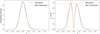 |
Fig. 1 Probability density function and ℓ1-norm for a Gaussian distribution (blue) and the non-Gaussian distribution (orange). On the left, we present the PDF for the two distributions, and on the right, we display the derived ℓ1-norm of these PDFs. The peak heights are the same for a Gaussian distribution, but this does not hold for a non-Gaussian PDF. |
2.4 Gaussian ℓ1-norm
We studied the anticipated wavelet ℓ1-norm expected from a Gaussian distribution. The generic shape of a wavelet ℓ1-norm obtained from a Gaussian PDF,
 (8)
(8)
with a mean µ = 0 and σ = 0.1 using the relation shown in Eq. (7) is demonstrated in Fig. 1.
The heights of the two peaks obtained for the wavelet ℓ1-norm for the Gaussian (solid blue line) distribution are equal, as expected. Because the Universe evolves, however, non-linearities develop, which means that the convergence field κ that we are interested in can no longer be modelled using a Gaussian model. These non-linearities would lead to an asymmetry that would also be evident from the peaks of the wavelet ℓ1-norm, which will no longer correspond. This is demonstrated in Fig. 1 for a testcase scenario, where we applied a non-linear exponential transformation to the Gaussian field to obtain a non-Gaussian field (solid orange line) and obtained the PDF and the ℓ1-norm. We emphasise that the usual way to extract this non-linear information is either by relying on heavy 𝒩-body simulations or by using an approximation, as was done in Tessore et al. (2023). With LDT, we now have a theoretically motivated way to obtain the PDF in the mildly non-linear regime, with which we show that we can also obtain the wavelet ℓ1-norm in the mildly non-linear regime.
3 Formalism of the large deviation theory
We applied the LDT to the convergence field. LDT, as explored in earlier works (Varadhan 1984), examines the rate at which the probabilities of specific events exponentially decrease as a key parameter of the problem varies. To derive the wavelet ℓ1-norm based on the LDT formalism, we first need to recapitulate how the PDF is obtained from the LDT formalism.
3.1 Large deviation theory for the matter field
The application of LDT to the field of Large Scale Structure cosmology has systematically been developed in recent years and is applied in the specific context of cosmic shear observations in this work. (Bernardeau & Reimberg 2016) clarified the application of the theory to the cosmological density field, establishing its link to earlier studies focused on cumulant calculations and modelling the matter PDF through perturbation theory and spherical collapse dynamics (Valageas 2002; Bernardeau et al. 2014b). Barthelemy et al. (2020) then provided an LDT-based prediction for the top-hat-filtered weak-lensing convergence PDF on mildly non-linear scales, building upon earlier work by (Bernardeau & Valageas 2000).
A more detailed derivation of the specific equations used is presented in the Appendix A. In this section, we recall the main equation with which we derive the wavelet ℓ1-norm prediction.
Application of LDT in cosmology involves three main steps. The first step is the derivation of the rate function, which is directly obtained from the first principles of cosmology. Using the contraction principle in the LDT formalism, we can connect the statistics of the late-time non-linear densities to the earlier-time density field when the most likely mapping between the two is known. Previous works have shown that assuming spherical collapse for this mapping provides us with a very accurate prediction for cosmic field PDF (density, velocity, convergence, etc.).
In particular, the result for convergence reads
 (9)
(9)
where P(κ) is the PDF of the convergence field κ, and ϕκ,θ is the cumulant generating function (CGF) of the field κ at angular scale θ. The derivation of the CGF in the above equation and the PDF from there is explained in more detail in the Appendix A.
3.2 Extension to wavelet coefficients
From the PDF, we can now compute the ℓ1-norm. As described in the Sect. 2, a wavelet can be written as a function of scaling functions. Although various wavelet filters exists in literature, we employed a function of concentric disks to construct the wavelet filter  .
.
The scaling function ξ is then given by a spherical top-hat filter and is given by
 (10)
(10)
where J1 is the first Bessel function of the first kind. This is applied, as shown in Eq. (5), to obtain our compensated filter. In Fig. 2 we show the compensated filter (solid black line) we used, which is given as a function of two scaling functions (solid orange and blue lines) at different scales.
We applied the LDT formalism described previously to the wavelet coefficients described in Eq. (5) and obtained the PDF of the wavelet coefficients  by using the scales θ1,θ2 = 2θ1 as
 (11)
(11)
We refer to the Appendix A for more details about the derivation of the CGF in the above equation and the resulting PDF. We emphasise that  is essentially the standard aperture mass defined on the convergence field using the difference of two top-hat filters, as was discussed previously.
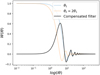 |
Fig. 2 Compensated filter (solid black line), derived through the difference of two top-hat filters at different scales, as described in Eqs. (5) and (10). The solid blue and orange lines represent the individual spherical filters obtained at radii θ1 and θ2 = 2θ1, respectively. For visualisation purposes, the compensated filter is multiplied by −1. |
3.3 Wavelet ℓ1-norm predicted via large deviation theory
In the previous sections, we showed that the LDT formalism can be applied to derive the PDF of the wavelet coefficients. We derive the wavelet ℓ1-norm from the PDF of the wavelet coefficients  here. This wavelet ℓ1-norm given in Eq. (6), which is the sum of the absolute values of the pixels in each bin, is equivalent to multiplying the counts/PDF value by the absolute value of the bin to which it corresponds, as given in Eq. (7). Extending this to the PDF of the wavelet coefficients from the LDT formalism, we obtain the final equation for bin i,
 (12)
(12)
As a first approximation, we assume that the PDF is Gaussian, which is the case when we consider large scales or early times in the standard model of cosmology. In the subsequent section, we first obtain the ℓ1-norm for a Gaussian case and then highlight the motivation to go beyond Gaussian models.
4 Comparing ℓ1-norm prediction to simulations
4.1 Measurements from simulation
To demonstrate the accuracy of the theory for realistic surveys, we compared our prediction results with fthe ull-sky simulations of Takahashi et al. (2017) to avoid additional errors from small-scale patch sizes. The simulations of Takahashi et al. (2017) provide full-sky lensing maps at a fixed cosmology3 each for two grid resolutions: 40962 and 8 1 922. The data sets include the full-sky maps at intervals of 150 h−1 comoving radial distance from redshifts z = 0.05–5.3. We used the simulated convergence maps that are directly provided as products of these simulations. The convergence maps were smoothed as a direct convolution of the convergence map with the wavelet filter at a given angular scale. After we obtained the filtered field, we measured the sum of the absolute values of the pixels of the smoothed κ mass map in linearly spaced bins of the range of κ to obtain the wavelet ℓ1-norm.
4.2 Obtaining the prediction
To obtain the prediction of the wavelet ℓ1-norm for each of the cosmologies used here, we first used CAMB (Lewis & Challinor 2011) to obtain the linear and non-linear (Halofit takahashi (Takahashi et al. 2012)) matter power spectra. We also used CAMB to obtain the comoving radial distances χ(z). The density CGF (Eq. (A.9)) was calculated for redshift slices between z = 0 and the source redshift zs using the full Halofit power spectrum as input. These projected CGFs were then rescaled by the measured variance  (see the Appendix A for more details), before going through an inverse Laplace transform to obtain the final PDF. This predicted PDF was used to derive the predicted wavelet ℓ1-norm as given in Eq. (12).
4.3 Validating the prediction with simulation
In Figures 3 and 4, we show the predicted wavelet ℓ1-norm and the one measured from the simulated convergence map for different source redshifts zs ≈ 1.2, 1.4, and 2.0 at θ = 20′ and for different scales θ = 15′, 18′, and 20′ at source redshift zs = 1.423, respectively. In the bottom panels, we show the residuals. For comparison, we display the PDF and the residuals of a Gaussian distribution (dash-dotted line) with the same mean and variance as the simulation. The Gaussian PDF was obtained using Eq. (8), and the ℓ1-norm was derived as explained previously in Eq. (12). In both plots, the x-axis for the residuals is scaled by the standard deviation. The shaded regions in the colours correspond to the 3σ region obtained from the error bars.
The error bars were obtained by taking the standard deviation of the values of the wavelet ℓ1-norm for ten different patches of the full-sky Takahashi map in each of the bins.
We first concentrated on the Gaussian curves. The Gaussian prediction is a clear mismatch, as expected, because the measurements show a clear asymmetry for the Gaussian model, which by definition is symmetric.
We then focused on the LDT prediction, which goes beyond the Gaussian regime. In this case, the agreement between the simulation and the predicted wavelet ℓ1-norm results is better at the percent level (which corresponds to the simulation error bars in the shaded area) within the 2σ region around zero on the x-axis. This demonstrates the predictive accuracy of the results derived from the LDT formalism. It is important to note that this 2σ specification refers to the range on the x-axis and does not represent error bars around the mean signal value.
These plots clearly show that LDT captures the asymmetry of the two peaks well and therefore providees valuable information about the non-Gaussianities. To better assess this aspect, we also show in Table 1 the cumulants obtained for the three scales at source redshift zs = 1.423. The cumulants shown here are the variance (σ2) and reduced skewness (S3), which, given that the mean convergence is zero, were obtained as
![Mathematical equation: ${\sigma ^2} = E\left[ {{\kappa ^2}} \right]$](/articles/aa/full_html/2024/11/aa50061-24/aa50061-24-eq27.png) (13)
(13)
![Mathematical equation: ${S_3} = {{E\left[ {{\kappa ^3}} \right]} \over {{\sigma ^4}}},$](/articles/aa/full_html/2024/11/aa50061-24/aa50061-24-eq28.png) (14)
(14)
where
![Mathematical equation: $E\left[ {{\kappa ^n}} \right] = \mathop \smallint \nolimits^ P(\kappa ){\kappa ^n}{\rm{d}}\kappa .$](/articles/aa/full_html/2024/11/aa50061-24/aa50061-24-eq29.png) (15)
(15)
Table 1 shows that the variance from the prediction and simulation for different scales matches perfectly, which we expect given the re-scaling by the power spectrum that we performed (see Appendix A). As expected from the formalism, the reduced skewness (S3) increases with decreasing smoothing scale. We also note that the ℓ1 -norm for the positive bins is not at all equal to the negative bins, suggesting how prominent the non-Gaussian features of the mass map are in this regime. Barthelemy et al. (2020) reported that the theoretical precision that can be achieved is constrained by the mixing of scales when integrating the density field along the line of sight since highly non-linear scales are not precisely captured by the spherical collapse formalism. Consequently, weak-lensing statistical measures are often approached through more phenomenologi-cal methods, such as halo models. These models are capable of incorporating baryonic physics, which becomes crucial at smaller scales, as highlighted by Mead et al. (2021). This is also evident in Figs. 3 and 4, where the level of accuracy increases at higher redshifts and higher smoothing scales. To bypass this issue, a rising approach is to use the so-called Bernardeau-Nishimichi-Taruya (BNT) transform (Bernardeau et al. 2014a), which enables more accurate theoretical predictions by narrowing the range of physical scales that contribute to the signal.
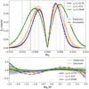 |
Fig. 3 Comparison of the predicted wavelet ℓ1 -norm to the simulations at different redshifts. Top panel: predicted (solid) ℓ1-norm as compared to measurements in simulation (dots) for an inner radius θ1 = 20′ and different source redshifts zs = 1.21,1.43 and 2.05, displayed with blue, orange, and green lines, respectively. The dash-dotted red lines show the Gaussian prediction for reference. The vertical dotted and dot-dashed lines correspond to the 1σ and 2σ regions around the mean of the |

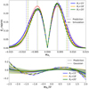 |
Fig. 4 Comparison of the predicted wavelet ℓ1 -norm to the simulations at different scales. Top panel: predicted (solid) ℓ1 -norm as compared to measurements in simulation (dots) for different inner radii θ1 = 15′, 18′, and 20′ and a single source redshift zs = 1.43, displayed with blue, orange, and green lines, respectively. The dash-dotted red lines show the Gaussian prediction for reference. The vertical dotted and dot-dashed lines correspond to the 1σ and 2σ regions around the mean of the |

Cumulants (standard deviation σ, skewness S3) obtained from the PDF from the LDT prediction and the values obtained from the Takahashi simulation at source redshift zs ≈ 2.05 for scales of 15, 18, and 20 arcminutes.
4.4 Cosmology dependence of the probability distribution function and the wavelet ℓ1 -norm
In this section, we explore the cosmological dependence of the predicted pdf of the wavelet coefficients and ℓ1-norm. We emphasise that because the wavelet decomposition is analogous to using an aperture mass map filtering, we henceforth also call the PDF of the wavelet coefficients the aperture mass PDF. From the equation of the rate function given in Eq. (A.7), the cosmology dependence of the aperture mass PDF in LDT enters through the scale dependence of the non-linear power-spectrum, the dynamics of the spherical collapse, and the lensing kernel. Moreover, the presence of massive neutrinos, if any, also affects the aperture mass as it enters the lensing kernel, as given in Eq. (3) by contributing to the total matter density budget. All of this inevitably means that the summary statistics are also cosmology-dependent. In the context of applying LDT to predict the wavelet ℓ1 -norm and PDFs, based on the equations introduced above, we assume that it should be able to efficiently capture the cosmology dependence. The cosmology dependence of the one-scale one-point convergence PDF was studied in detail by Boyle et al. (2021), who showed that LDT captures the cosmology dependence very accurately. We extend this study for the case of the PDF of the wavelet coefficients and the wavelet ℓ1 -norm of aperture mass maps. As for the one- scale case, the rate function for the multi- scale also depends on the variance and the dynamics of the spherical collapse, which means that the PDF of the wavelet coefficients would also be expected to depend (similarly) on the cosmology. Additionally, because the wavelet ℓ1 -norm is directly dependent on the PDF, we could naively expect it to depend on the cosmology as well, and encapsulate the dependence.
We are interested in obtaining the derivatives with respect to cosmological parameters. We therefore need a simulation suite that is available for different cosmologies. For this, we used the cosmological massive neutrino simulations (MassiveNus) (Liu et al. 2018) suite to determine how well the theory captures the dependence on cosmology. These simulations were released by the Columbia Lensing Group4. The MassiveNuS simulations encompass 101 different cosmological models at source redshifts zs = 0.5, 1.0, 1.5, 2.0, and 2.5 by varying three parameters: the neutrino mass sum Mv, the total matter density Ωm, and the primordial power spectrum amplitude As. For each redshift, 10000 distinct map realisations are generated through random rotation and translation of the initial n-body box and are then stitched together to reconstruct pseudo-independent light cones that are unlikely to cross the same structures. Each k map contains 5122 pixels, covering a total angular area of 12.25 square degrees, spanning a range of ℓ ∈ [100,37 000] with a pixel resolution of 0.4 arcminutes. The wavelet ℓ1 -norm is measured using the same process as described previously in Sect. 4.1. Additionally, the measurement of the PDF is derived from the histogram of the binned and smoothed map. To obtain the derivatives, we used a model with the parameters Ωm = 0.30, As = 2.1 × 10⁻⁹, and Mv = 0.0 eV as the fiducial model (model 1b in Liu et al. (2018)) and obtained the derivatives of the PDF for each of the parameters. The different parameters are shown in Table 2. The outcomes are illustrated in Figures 5–6. For the derivative with respect to Mv, we employed a model with the same Ωm and As values, but with Mv = 0.0, eV and then computed the derivative. However, it is important to note that due to resolution and finite volume effects, the simulation power spectrum of the convergence maps exhibits a deficit in power at high ℓ, which strongly affects our results because of the scales we considered, and at low ℓ, which invites caution when choosing our largest scales. We typically tried to maintain a factor of 20 between the physical scale of the box and the largest physical scale probed by our filters.
Figures 5 and 6 clearly show that the prediction effectively captures the changes in cosmology and agrees well with the results. The error bars were obtained by taking the error of the mean of 3000 simulations, which were also used to obtain the mean of the measurements.
As demonstrated in Boyle et al. (2021) for the case of a one-cell PDF, our results here demonstrate that the theory captures the effects of adding massive neutrinos to cosmology well and extend the results to the PDF of the wavelet coefficients as well.
Cosmological parameters used to obtain the derivatives of the PDF.
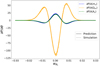 |
Fig. 5 Derivative of the PDF with respect to Mv (blue), Ωm (orange), and As (green). The solid lines show the derivatives obtained from the prediction, and the dotted lines show the derivatives from the simulation. It is obtained at source redshift zs = 2 and inner radius θ1 = 22.5′. The results for the simulation are obtained from the MassiveNus simulation suite by averaging the results over 10 000 simulations. |
4.5 Reproducible research
In the spirit of open research, the code for reproducing the plots in this paper is available at github. The part of this Python code that computed the aperture mass/wavelet coefficient PDF was inspired by the public Mathematica code L2DT used in Barthelemy et al. (2021).
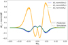 |
Fig. 6 Derivative of the wavelet ℓ1 -norm with respect to Mv (blue), Ωm (orange), and As (green). The solid lines show the derivatives obtained from the prediction, and the dotted lines show the derivatives from the simulation. The predicted wavelet ℓ1 -norm is derived from the predicted PDF, as was explained in previous sections. It is obtained at source red-shift zs = 2 and inner radius θ1 = 22.5′. The results for the simulation are obtained from the MassiveNus simulation suite by averaging the results over 10 000 simulations. |
5 Discussion and conclusions
We have used the LDT to build upon previous work by Barthelemy et al. (2021) and introduced a formalism to predict the ℓ1 -norm of the wavelet coefficients of the lensing field and their cosmological dependence for any given redshift and scales as long as they are in the mildly non-linear regime. The approach of Barthelemy et al. (2021) incorporated geometric and time-evolution aspects within the light cone by considering that the correlations of the underlying matter density field along the line of sight are negligible compared to transverse directions. This Limber approximation enabled us to treat redshift slices as statistically independent. We found that the most likely non-linear dynamics of the matter density field filtered in concentric disks can be well approximated for small variances by the cylindrical collapse model, thus allowing us to apply LDT in this context. From there, because the wavelet ℓ1 -norm can be directly related to the multi-scale one-point statistics of the convergence, we showedr that a theory-based prediction for the wavelet ℓ1 -norm is tractable.
The robust validation of our predictions against the simulations is shown in Figs. 4 and 3. This highlighted the reliability and applicability of our theoretical framework. Specifically, our theory aligns with the simulations within a percent-level accuracy in the examined range of source redshifts zs ≈ 1–2 and angular scales θ1 ≈ 15–20. This quantitative assessment affirms the predictive precision of our model. Smaller scales or lower redshifts would clearly lead to a larger departure between simulations and theory.
Figure 6 further emphasises the cosmological dependencies and the very good performance of the theoretical prediction when compared with that of the simulation. Since the simulations validated the theoretical predictions, this suggests that our model can be applied to investigate a broad range of cosmological parameters while bypassing the need for high-cost computing resources and providing a theoretical tool for cosmology inference that is robust and fast, without loss of quality. This paves the way for a more comprehensive and faster forecast analysis based on theory without having to rely on expensive numerical simulations. In addition, we noted in Figures 5 and 6 that there is numerical noise in the simulation results (fitted lines). This can lead to biases in parameter estimates when using the simulation data. A theory-based approach has the added benefit of reducing the artificial biases in the parameter inference, which was also noted in Boyle et al. (2021).
Another point to be noted is that although lower source redshifts are expected to generate more non-Gaussian information, this also pushes the model deeper into the non-linear regime. This effect can be mitigated by adjusting the smoothing scale accordingly. We also emphasise the usefulness of the wavelet coefficients of the convergence maps, instead of directly using the convergence maps or the shear maps. Convergence maps already reduce computational expense through a more compressed lensing signal when compared to the shear map. However, the use of the wavelet scales and/or coefficients provides us with a multi-scale analysis method that is well suited to constraining the cosmology.
Moreover, wavelet coefficients are invariant under the mass sheet degeneracy, which renders the link to the measured shear data more straightforward.
More generally, one of the issues with the theoretical modelling of weak lensing we currently face is the mixing of (nonlinear) scales that is inherent in such quantities projected along the past light cone and makes standard perturbative approaches inaccurate even at relatively large angular scales. (Bernardeau et al. 2014a) To overcome this issue, an emerging method is the BNT transform, which allows more precise theoretical predictions by reducing the range of physical scales that contribute to the signal. This can be applied in our context and enables even more accurate predictions for analysing tomographic surveys. An investigation of the performance of this approach is left for future works, together with the impact of systematics, which would require us to devise specific simulated data, as well as additional theoretical development.
We conclude that the novel approach for obtaining the theoretical prediction of the wavelet ℓ1-norm summary statistic proposed here presents several advantages in the realm of cosmological parameter inference: (i) it provides a fast (about one minute) calculation, (ii) it does not rely on a heavy numerical simulation, (iii) it captures the cosmology dependence well, and (iv) the wavelet ℓ1 -norm might lead to competitive or even tighter constraints, as demonstrated by previous works. This promising method might enable a comprehensive multi-scale analysis of cosmic shear datasets in the mildly non-linear regime.
Data availability
The code for reproducing the plots in this paper is available at https://github.com/vilasinits/LDT_2cell_l1_norm
Acknowledgements
This work was funded by the TITAN ERA Chair project (contract no. 101086741) within the Horizon Europe Framework Program of the European Commission, and the Agence Nationale de la Recherche (ANR-22-CE31-0014-01 TOSCA and ANR-18-CE31-0009 SPHERES). A.B.’s work is supported by the ORIGINS excellence cluster. We thank Jia Liu and the Columbia Lensing group http://columbialensing.org) for making the MassiveNus (Liu et al. 2018) simulations available. The creation of these simulations is supported through grants NSF AST-1210877, NSF AST-140041, and NASA ATP-80NSSC18K1093. We thank New Mexico State University (USA) and Instituto de Astrofisica de Andalucia CSIC (Spain) for hosting the Skies & Universes site for cosmological simulation products. We also thank C. Uhlemann, O. Friedrich, Lina Castiblanco, and Martin Kilbinger for insightful discussions.
Appendix A Large Deviation Theory
A.1 LDT for the matter field
The computations detailed in this section draw heavily from the formulations provided in Boyle et al. (2021) and Barthelemy et al. (2021). Here, we will succinctly restate the key equations and direct the reader to the comprehensive treatments in Boyle et al. (2021), Barthelemy et al. (2021), and Reimberg & Bernardeau (2018).
The LDT, as explored in earlier works Varadhan (1984), examines the rate at which the probabilities of specific events diminish as a key parameter of the problem undergoes variation. Widely applied in various mathematical and theoretical physics domains, this theory is particularly prominent in statistical physics, covering both equilibrium and non-equilibrium systems. For a detailed overview, readers are referred to Touchette (2009).
The Large Deviation Principle (LDP) in the domain of Large Scale Structure cosmology has been systematically developed in recent years and will be applied in the specific context of cosmic shear observations in this work. Bernardeau & Reimberg (2016) clarified the application of the theory to the cosmological density field, establishing its link to earlier studies focused on cumulant calculations and modelling the matter PDF through perturbation theory and spherical collapse dynamics (Valageas (2002); Bernardeau et al. (2014b)). Barthelemy et al. (2020) provided an LDT-based prediction for the top-hat-filtered weak-lensing convergence PDF on mildly nonlinear scales, building upon earlier work by Bernardeau & Valageas (2000).
The LDP applied to the matter density field relies on three key aspects:
Defining a rate function for variables in the initial field configuration. In this context, we opt for Gaussian initial conditions and establish their covariance matrix.
Describing the relationship between the initial field configuration (representing the mass profile) and the resulting mass profile, based on 2D cylindrical collapse or a suitable approximation.
Using these foundations to express observable quantities, like a map created with a specific filter, as functional expressions that depend on both the final and initial mass profile.
A LDP for matter densities at multiple scales (indexed by i)  , 1 ≤ i ≤ N with joint PDF
  is satisfied if the following limit exists
![Mathematical equation: ${\psi _{\left\{ {\rho _i^} \right\}}}\left( {\left\{ {\rho _i^} \right\}} \right) = - \mathop {\lim }\limits_{ \to 0} \log \left[ {{{\cal P}_}\left( {\left\{ {\rho _i^} \right\}} \right)} \right].$](/articles/aa/full_html/2024/11/aa50061-24/aa50061-24-eq33.png) (A.1)
(A.1)
If such limit exists,  is called the rate function.
Here, ϵ is a driving parameter, indicating the set of random variables linked to a specific evolutionary process. For the matter density field at a single scale, this parameter reflects its variance, marking time from initial stages to later times. In joint statistics involving concentric disks of matter, the common driving parameter can be selected as the variance at any radius or scale. This consistency arises because all variances behave the same as they approach zero. In this limit, they directly scale with the square of the growth rate of structure in the linear regime.
If LDP holds for the random variable ρi, then Varadhan’s theorem allows us to connect its Scaled Cumulant Generating Function (SCGF)  to the rate function
  through a Legendre-Fenchel transform
![Mathematical equation: ${\varphi _{\left\{ {{\rho _i}} \right\}}}\left( {\left\{ {{\lambda _i}} \right\}} \right) = \mathop {\sup }\limits_{\left\{ {{\rho _i}} \right\}} \left[ {\mathop \sum \limits_i {\lambda _i}{\rho _i} - {\psi _{\left\{ {{\rho _i}} \right\}}}\left( {\left\{ {{\rho _i}} \right\}} \right)} \right].$](/articles/aa/full_html/2024/11/aa50061-24/aa50061-24-eq37.png) (A.2)
(A.2)
This Legendre-Fenchel transform reduces to Legendre transform if the rate function is convex
 (A.3)
(A.3)
where λi and ρi are one by one related via the stationary condition
 (A.4)
(A.4)
Another consequence of the large-deviation principle is the so-called contraction principle. This principle suggests that when dealing with a set of random variables τi following a large deviation principle LDP and connected to ρi through the continuous mapping f, the rate function of ρi can be determined as follows
 (A.5)
(A.5)
In more tangible terms, this statement suggests that an uncommon change in the behavior of ρi is predominantly influenced by the most probable variation among all unlikely changes in τi.
In the context of cosmology, if we take ρk to denote the late-time densities, then  , the most likely initial field configuration, is obtained through the most probable mapping between the linear and late-time fields. In 2D, this most likely dynamics is given by cylindrical collapse, which is known to be well-fitted by
 (A.6)
(A.6)
The choice of v as 1.4 is made to match the calculated value of the third-order skewness of the matter density contrast in cylinders from perturbation theory, as presented in Uhlemann et al. (2018). The standard result for spherical collapse dynamics in 1 to 3D can be found in Mukhanov (2005).
Now that we know the most likely connection between initial conditions and the late-time field configuration, we can compute the rate function for the late-time density field. It is expressed as follows
 (A.7)
(A.7)
Here,  is the driving parameter and is determined by the variance within the largest disk R1. Ξkj is the inverse covariance matrix between the linear density field inside the initial disks of radii
  .
.
A.2 Applying LDT to aperture mass PDF
Following Barthelemy et al. (2021), an accurate modelling of the top-hat smoothed weak lensing convergence can be obtained (Limber) approximating that the convergence field is an assembly of statistically independent infinitely long cylinders of the underlying matter density contrast. Those cylinders are centred on slices along the line of sight, and they reduce to those 2D slices as illustrated in Fig. A.1. This means that the cumulants can be written as
 (A.8)
(A.8)
where  is a random variable that defines the slope between two concentric disks of radii
  and
and  at comoving radial distance χ. This simplifies the problem greatly, now having to calculate just the one-point statistics related to the density slope within each two-dimensional slice along the line of sight.
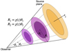 |
Fig. A.1 Schematic view of the procedure to obtain the aperture mass map following (Barthelemy et al. 2021). The projected quantities can be inferred as a superposition of the underlying 3D density field along the line of sight. |
As is explained in Appendix A of Barthelemy et al. (2021), the choice of driving parameter is not predicted by theory and is left as a free parameter. However, when computing the joint statistics of the density fields at different scales, this choice prevents us from imposing correct quadratic contributions in the CGF. This leads us to use the full non-linear prescription coming from the Halofit to model the non-linear covariance. In this paper, we use the Halofit-Takahashi version Takahashi et al. (2012) to compute the covariances.
Now using Eq. (A.3), and Eq. (A.7), and since we need the density slope between two concentric disks, we get the SCGF as
 (A.9)
(A.9)
To ensure that this choice does not lead to any discrepancies with the numerical simulations, we also rescale the projected CGF given in Eq. (A.3) with the measured variance  instead of the one computed from Halofit
  as is given below
 (A.10)
Once the CGF of individual slices is obtained, we can use Eq. (A.8) to get the CGF (the details of this derivation is given in Barthelemy et al. (2021)) of the lensing aperture mass as
 (A.11)
After calculating the CGF, the inverse Laplace transform can be used to obtain the convergence PDF
 (A.12)
As described in more detail in Barthelemy et al. (2021), the inverse Laplace transform we need to perform assumes that the CGF is defined in the complex plane along the path of integration. Unfortunately, the use of numerical results for the matter power spectra prevents us to perform this continuation from the real axis. As a result, we use an informed fit of the numerical CGF along the real axis with a finite number of coefficients that we then extend to the complex plane. This allows to perform the previous integral.
Now that we have a PDF of the aperture mass map P(Map)/alternatively the wavelet coefficients, we could use that to obtain the wavelet ℓ1-norm using the Eq. (12) as demonstrated in the Sect. 3.3.
References
- Ajani, V., Peel, A., Pettorino, V., et al. 2020, Phys. Rev. D, 102, 103531 [Google Scholar]
- Ajani, V., Starck, J.-L., & Pettorino, V. 2021, A&A, 645, L11 [NASA ADS] [CrossRef] [EDP Sciences] [Google Scholar]
- Ajani, V., Harnois-Déraps, J., Pettorino, V., & Starck, J.-L. 2023, A&A, 672, L10 [NASA ADS] [CrossRef] [EDP Sciences] [Google Scholar]
- Bacon, D. J., Refregier, A. R., & Ellis, R. S. 2000, MNRAS, 318, 625 [NASA ADS] [CrossRef] [Google Scholar]
- Bartelmann, M., & Maturi, M. 2017, Scholarpedia, 12, 32440 [NASA ADS] [CrossRef] [Google Scholar]
- Barthelemy, A., Codis, S., Uhlemann, C., Bernardeau, F., & Gavazzi, R. 2020, MNRAS, 492, 3420 [Google Scholar]
- Barthelemy, A., Codis, S., & Bernardeau, F. 2021, MNRAS, 503, 5204 [Google Scholar]
- Bernardeau, F., & Reimberg, P. 2016, Phys. Rev. D, 94, 063520 [NASA ADS] [CrossRef] [Google Scholar]
- Bernardeau, F., & Valageas, P. 2000, A&A, 364, 1 [NASA ADS] [Google Scholar]
- Bernardeau, F., Colombi, S., Gaztañaga, E., & Scoccimarro, R. 2002, Phys. Rep., 367, 1 [Google Scholar]
- Bernardeau, F., Nishimichi, T., & Taruya, A. 2014a, MNRAS, 445, 1526 [Google Scholar]
- Bernardeau, F., Pichon, C., & Codis, S. 2014b, Phys. Rev. D, 90, 103519 [NASA ADS] [CrossRef] [Google Scholar]
- Boyle, A., Uhlemann, C., Friedrich, O., et al. 2021, MNRAS, 505, 2886 [NASA ADS] [CrossRef] [Google Scholar]
- Cheng, S., & Ménard, B. 2021, MNRAS, 507, 1012 [NASA ADS] [CrossRef] [Google Scholar]
- Euclid Collaboration (Deshpande, A. C., et al.) 2024, A&A, 684, A138 [NASA ADS] [CrossRef] [EDP Sciences] [Google Scholar]
- Fageot, J., Bostan, E., & Unser, M. 2014, in 2014 IEEE International Conference on Image Processing (ICIP), 6096 [CrossRef] [Google Scholar]
- Gatti, M., Chang, C., Friedrich, O., et al. 2020, MNRAS, 498, 4060 [Google Scholar]
- Giblin, B., Heymans, C., Harnois-Déraps, J., et al. 2018, MNRAS, 480, 5529 [Google Scholar]
- Giné, E., Mason, D. M., & Zaitsev, A. Y. 2003, Annal. Probab., 31, 719 [Google Scholar]
- Harnois-Déraps, J., Giblin, B., & Joachimi, B. 2019, A&A, 631, A160 [NASA ADS] [CrossRef] [EDP Sciences] [Google Scholar]
- Heymans, C., Van Waerbeke, L., Miller, L., et al. 2012, MNRAS, 427, 146 [Google Scholar]
- Hildebrandt, H., Viola, M., Heymans, C., et al. 2017, MNRAS, 465, 1454 [Google Scholar]
- Hildebrandt, H., van den Busch, J. L., Wright, A. H., et al. 2021, A&A, 647, A124 [EDP Sciences] [Google Scholar]
- Huber, P. J. 1987, Comput. Stat. Data Anal., 5, 255 [CrossRef] [Google Scholar]
- Huterer, D. 2010, Gen. Relativ. Gravit., 42, 2177 [CrossRef] [Google Scholar]
- Ingoglia, L., Covone, G., Sereno, M., et al. 2022, MNRAS, 511, 1484 [NASA ADS] [CrossRef] [Google Scholar]
- Ivezic, Ž., Kahn, S. M., Tyson, J. A., et al. 2019, ApJ, 873, 111 [NASA ADS] [CrossRef] [Google Scholar]
- Jeffrey, N., Lanusse, F., Lahav, O., & Starck, J.-L. 2020, MNRAS, 492, 5023 [Google Scholar]
- Kaiser, N., Wilson, G., & Luppino, G. A. 2000, ApJ Letters [arXiv:astro-ph/0003338] [Google Scholar]
- Kilbinger, M. 2015, Rep. Prog. Phys., 78, 086901 [Google Scholar]
- Kilbinger, M. 2018, arXiv e-prints [arXiv:1807.08249] [Google Scholar]
- Kratochvil, J. M., Lim, E. A., Wang, S., et al. 2012, Phys. Rev. D, 85, 103513 [Google Scholar]
- Kruse, G., & Schneider, P. 1999, MNRAS, 302, 821 [Google Scholar]
- Laureijs, R., Amiaux, J., Arduini, S., et al. 2011, arXiv e-prints [arXiv:1110.3193] [Google Scholar]
- Leonard, A., Pires, S., & Starck, J.-L. 2012, MNRAS, 423, 3405 [NASA ADS] [CrossRef] [Google Scholar]
- Lesgourgues, J., & Pastor, S. 2012, Adv. High Energy Phys., 2012, 1 [CrossRef] [Google Scholar]
- Lewis, A., & Challinor, A. 2011, Astrophysics Source Code Library [record ascl:1102.026] [Google Scholar]
- Li, Z., Liu, J., Zorrilla Matilla, J. M., & Coulton, W. R. 2019, Phys. Rev. D, 99, 063527 [NASA ADS] [CrossRef] [Google Scholar]
- Lin, C.-A., & Kilbinger, M. 2015, A&A, 583, A70 [NASA ADS] [CrossRef] [EDP Sciences] [Google Scholar]
- Liu, J., & Madhavacheril, M. S. 2019, Phys. Rev. D, 99, 083508 [Google Scholar]
- Liu, J., Petri, A., Haiman, Z., et al. 2015a, Phys. Rev. D, 91, 063507 [Google Scholar]
- Liu, X., Pan, C., Li, R., et al. 2015b, MNRAS, 450, 2888 [Google Scholar]
- Liu, J., Bird, S., Matilla, J. M. Z., et al. 2018, J. Cosmol. Astropart. Phys., 2018, 049 [Google Scholar]
- Loureiro, A., Whiteaway, L., Sellentin, E., et al. 2023, Open J. Astrophys., 6, 6 [CrossRef] [Google Scholar]
- Mandelbaum, R. 2018, ARA&A, 56, 393 [Google Scholar]
- Mandelbaum, R., & Collaboration, H. S.-C. H. 2017, AAS Meeting Abstracts, 229, 226 [NASA ADS] [Google Scholar]
- Martinet, N., Bartlett, J. G., Kiessling, A., & Sartoris, B. 2015, A&A, 581, A101 [NASA ADS] [CrossRef] [EDP Sciences] [Google Scholar]
- Mead, A. J., Brieden, S., Tröster, T., & Heymans, C. 2021, MNRAS, 502, 1401 [Google Scholar]
- Mellier, Y. 1999, ARA&A, 37, 127 [NASA ADS] [CrossRef] [Google Scholar]
- Mukhanov, V. 2005, Physical Foundations of Cosmology (Cambridge: Cambridge University Press) [CrossRef] [Google Scholar]
- Munshi, D., Valageas, P., van Waerbeke, L., & Heavens, A. 2008, Phys. Rep., 462, 67 [NASA ADS] [CrossRef] [Google Scholar]
- Parroni, C., Cardone, V. F., Maoli, R., & Scaramella, R. 2020, A&A, 633, A71 [NASA ADS] [CrossRef] [EDP Sciences] [Google Scholar]
- Peebles, P. J. E. 1980, The Large-scale Structure of the Universe (Princeton: Princeton University Press) [Google Scholar]
- Peel, A., Lin, C.-A., Lanusse, F., et al. 2017, A&A, 599, A79 [NASA ADS] [CrossRef] [EDP Sciences] [Google Scholar]
- Peel, A., Pettorino, V., Giocoli, C., Starck, J.-L., & Baldi, M. 2018, A&A, 619, A38 [NASA ADS] [CrossRef] [EDP Sciences] [Google Scholar]
- Petri, A. 2016, Astron. Comput., 17, 73 [NASA ADS] [CrossRef] [Google Scholar]
- Reimberg, P., & Bernardeau, F. 2018, Phys. Rev. D 97, 032013 [CrossRef] [Google Scholar]
- Rizzato, M., Benabed, K., Bernardeau, F., & Lacasa, F. 2019, MNRAS, 490, 4688 [NASA ADS] [CrossRef] [Google Scholar]
- Schneider, P., van Waerbeke, L., Kilbinger, M., & Mellier, Y. 2002, A&A, 396, 1 [NASA ADS] [CrossRef] [EDP Sciences] [Google Scholar]
- Semboloni, E., Schrabback, T., van Waerbeke, L., et al. 2011, MNRAS, 410, 143 [Google Scholar]
- Shi, X., Schneider, P., & Joachimi, B. 2011, A&A, 533, A48 [NASA ADS] [CrossRef] [EDP Sciences] [Google Scholar]
- Starck, J. L., Pires, S., & Réfrégier, A. 2006, A&A, 451, 1139 [NASA ADS] [CrossRef] [EDP Sciences] [Google Scholar]
- Starck, J.-L., Murtagh, F., & Fadili, J. 2015, Sparse Image and Signal Processing: Wavelets and Related Geometric Multiscale Analysis, 2nd edn. (Cambridge: Cambridge University Press), 1 [Google Scholar]
- Starck, J. L., Themelis, K. E., Jeffrey, N., Peel, A., & Lanusse, F. 2021, A&A, 649, A99 [NASA ADS] [CrossRef] [EDP Sciences] [Google Scholar]
- Takada, M., & Jain, B. 2004, MNRAS, 348, 897 [Google Scholar]
- Takahashi, R., Sato, M., Nishimichi, T., Taruya, A., & Oguri, M. 2012, ApJ, 761, 152 [Google Scholar]
- Takahashi, R., Hamana, T., Shirasaki, M., et al. 2017, ApJ, 850, 24 [Google Scholar]
- Tessore, N., Loureiro, A., Joachimi, B., von Wietersheim-Kramsta, M., & Jeffrey, N. 2023, Open J. Astrophys., 6, 11 [NASA ADS] [CrossRef] [Google Scholar]
- Touchette, H. 2009, Phys. Rep., 478, 1 [NASA ADS] [CrossRef] [Google Scholar]
- Troxel, M., & Ishak, M. 2015, Phys. Rep., 558, 1 [NASA ADS] [CrossRef] [Google Scholar]
- Uhlemann, C., Pichon, C., Codis, S., et al. 2018, MNRAS, 477, 2772 [NASA ADS] [CrossRef] [Google Scholar]
- Valageas, P. 2002, A&A, 382, 412 [NASA ADS] [CrossRef] [EDP Sciences] [Google Scholar]
- Varadhan, S. R. S. 1984, Large Deviations and Applications (USA: Society for Industrial and Applied Mathematics) [CrossRef] [Google Scholar]
- Waerbeke, L. V., Mellier, Y., Erben, T., et al. 2000, A&A, 358, 30 [NASA ADS] [Google Scholar]
- Weinberg, D. H., Mortonson, M. J., Eisenstein, D. J., et al. 2013, Phys. Rep., 530, 87 [Google Scholar]
Code publicly available at GitHub: https://github.com/vilasinits/LDT_2cell_l1_norm
In the literature, the common practice has been to use a non-normalised version of the ℓ1-norm, but to facilitate comparison with prediction and simulation, we chose to normalise this quantity. For the sake of simplicity, we call it ℓ1-norm.
All Tables
Cumulants (standard deviation σ, skewness S3) obtained from the PDF from the LDT prediction and the values obtained from the Takahashi simulation at source redshift zs ≈ 2.05 for scales of 15, 18, and 20 arcminutes.
All Figures
|
Fig. 1 Probability density function and ℓ1-norm for a Gaussian distribution (blue) and the non-Gaussian distribution (orange). On the left, we present the PDF for the two distributions, and on the right, we display the derived ℓ1-norm of these PDFs. The peak heights are the same for a Gaussian distribution, but this does not hold for a non-Gaussian PDF. |
| In the text | |
|
Fig. 2 Compensated filter (solid black line), derived through the difference of two top-hat filters at different scales, as described in Eqs. (5) and (10). The solid blue and orange lines represent the individual spherical filters obtained at radii θ1 and θ2 = 2θ1, respectively. For visualisation purposes, the compensated filter is multiplied by −1. |
| In the text | |
|
Fig. 3 Comparison of the predicted wavelet ℓ1 -norm to the simulations at different redshifts. Top panel: predicted (solid) ℓ1-norm as compared to measurements in simulation (dots) for an inner radius θ1 = 20′ and different source redshifts zs = 1.21,1.43 and 2.05, displayed with blue, orange, and green lines, respectively. The dash-dotted red lines show the Gaussian prediction for reference. The vertical dotted and dot-dashed lines correspond to the 1σ and 2σ regions around the mean of the |
| In the text | |
|
Fig. 4 Comparison of the predicted wavelet ℓ1 -norm to the simulations at different scales. Top panel: predicted (solid) ℓ1 -norm as compared to measurements in simulation (dots) for different inner radii θ1 = 15′, 18′, and 20′ and a single source redshift zs = 1.43, displayed with blue, orange, and green lines, respectively. The dash-dotted red lines show the Gaussian prediction for reference. The vertical dotted and dot-dashed lines correspond to the 1σ and 2σ regions around the mean of the |
| In the text | |
|
Fig. 5 Derivative of the PDF with respect to Mv (blue), Ωm (orange), and As (green). The solid lines show the derivatives obtained from the prediction, and the dotted lines show the derivatives from the simulation. It is obtained at source redshift zs = 2 and inner radius θ1 = 22.5′. The results for the simulation are obtained from the MassiveNus simulation suite by averaging the results over 10 000 simulations. |
| In the text | |
|
Fig. 6 Derivative of the wavelet ℓ1 -norm with respect to Mv (blue), Ωm (orange), and As (green). The solid lines show the derivatives obtained from the prediction, and the dotted lines show the derivatives from the simulation. The predicted wavelet ℓ1 -norm is derived from the predicted PDF, as was explained in previous sections. It is obtained at source red-shift zs = 2 and inner radius θ1 = 22.5′. The results for the simulation are obtained from the MassiveNus simulation suite by averaging the results over 10 000 simulations. |
| In the text | |
|
Fig. A.1 Schematic view of the procedure to obtain the aperture mass map following (Barthelemy et al. 2021). The projected quantities can be inferred as a superposition of the underlying 3D density field along the line of sight. |
| In the text | |
Current usage metrics show cumulative count of Article Views (full-text article views including HTML views, PDF and ePub downloads, according to the available data) and Abstracts Views on Vision4Press platform.
Data correspond to usage on the plateform after 2015. The current usage metrics is available 48-96 hours after online publication and is updated daily on week days.
Initial download of the metrics may take a while.