| Issue |
A&A
Volume 679, November 2023
|
|
|---|---|---|
| Article Number | A61 | |
| Number of page(s) | 18 | |
| Section | Cosmology (including clusters of galaxies) | |
| DOI | https://doi.org/10.1051/0004-6361/202346888 | |
| Published online | 07 November 2023 | |
Forecasting the power of higher order weak-lensing statistics with automatically differentiable simulations
1
Université Paris Cité, Université Paris-Saclay, CEA, CNRS, AIM, 91191 Gif-sur-Yvette, France
e-mail: This email address is being protected from spambots. You need JavaScript enabled to view it.
2
Université Paris-Saclay, Université Paris Cité, CEA, CNRS, AIM, 91191 Gif-sur-Yvette, France
3
Center for Computational Astrophysics, Center for Computational Mathematics, Flatiron Institute, New York, NY 10010, USA
4
Lawrence Berkeley National Laboratory, 1 Cyclotron Road, Berkeley, 94720 CA, USA
5
Department of Astrophysical Sciences, Princeton University, Princeton, NJ 08544, USA
6
School of Mathematics, Statistics and Physics, Newcastle University, Herschel Building, NE1 7RU Newcastle-upon-Tyne, UK
Received:
12
May
2023
Accepted:
7
August
2023
Abstract
Aims. We present the fully differentiable physical Differentiable Lensing Lightcone (DLL) model, designed for use as a forward model in Bayesian inference algorithms that require access to derivatives of lensing observables with respect to cosmological parameters.
Methods. We extended the public FlowPM N-body code, a particle-mesh N-body solver, while simulating the lensing lightcones and implementing the Born approximation in the Tensorflow framework. Furthermore, DLL is aimed at achieving high accuracy with low computational costs. As such, it integrates a novel hybrid physical-neural (HPN) parameterization that is able to compensate for the small-scale approximations resulting from particle-mesh schemes for cosmological N-body simulations. We validated our simulations in the context of the Vera C. Rubin Observatory’s Legacy Survey of Space and Time (LSST) against high-resolution κTNG-Dark simulations by comparing both the lensing angular power spectrum and multiscale peak counts. We demonstrated its ability to recover lensing Cℓ up to a 10% accuracy at ℓ = 1000 for sources at a redshift of 1, with as few as ∼0.6 particles per Mpc h−1. As a first-use case, we applied this tool to an investigation of the relative constraining power of the angular power spectrum and peak counts statistic in an LSST setting. Such comparisons are typically very costly as they require a large number of simulations and do not scale appropriately with an increasing number of cosmological parameters. As opposed to forecasts based on finite differences, these statistics can be analytically differentiated with respect to cosmology or any systematics included in the simulations at the same computational cost of the forward simulation.
Results. We find that the peak counts outperform the power spectrum in terms of the cold dark matter parameter, Ωc, as well as on the amplitude of density fluctuations, σ8, and the amplitude of the intrinsic alignment signal, AIA.
Key words: methods: statistical / cosmology: large-scale structure of Universe / gravitational lensing: weak
© The Authors 2023
 Open Access article, published by EDP Sciences, under the terms of the Creative Commons Attribution License (https://creativecommons.org/licenses/by/4.0), which permits unrestricted use, distribution, and reproduction in any medium, provided the original work is properly cited.
This article is published in open access under the Subscribe to Open model. This email address is being protected from spambots. You need JavaScript enabled to view it. to support open access publication.
1. Introduction
Weak gravitational lensing by large-scale structures (LSS) is one of the key probes used to test cosmological models and gain insights into the constituents of the Universe. Upcoming stage IV surveys, such as the Legacy Survey of Space and Time (LSST) of the Vera C. Rubin Observatory Ivezić et al. (2019), Nancy Grace Roman Space Telescope (Spergel et al. 2015), and the Euclid Mission (Laureijs et al. 2011), will provide measurements for billions of galaxy shapes with unprecedented accuracy. This development, in turn, will lead to tighter constraints on dark energy models (e.g., Mandelbaum et al. 2018).
With the increased statistical power of these surveys comes the question of their optimal analysis. Traditional cosmological analyses rely on measurements of the two-point statistics: either the shear two-point correlation functions or its Fourier transform, that is, the lensing power spectrum. However, the two-point statistics are only optimal for Gaussian fields and do not fully capture the non-Gaussian information imprinted in the lensing signal at the scales that future surveys will be able to access (e.g., information encoded in the peaks and in the filamentary features of the matter distribution).
This has led to the introduction of a number of higher order statistics to access the non-Gaussian information from weak-lensing data: the weak-lensing one-point probability distribution function (PDF, Liu & Madhavacheril 2019; Uhlemann et al. 2020; Boyle et al. 2021), lensing peak counts (Liu et al. 2015a,b; Lin & Kilbinger 2015; Kacprzak et al. 2016; Peel et al. 2017; Shan et al. 2018; Martinet et al. 2018; Ajani et al. 2020; Harnois-Déraps et al. 2022; Zürcher et al. 2022), Minkowski functionals (Kratochvil et al. 2012; Petri et al. 2013), moments of mass maps (Gatti et al. 2022), wavelet and scattering transforms (Ajani et al. 2021; Cheng & Ménard 2021), and three-point statistics (Takada & Jain 2004; Semboloni et al. 2011; Rizzato et al. 2019; Halder et al. 2021).
More recently, machine learning-based methods that broadly fall in the category of simulation-based inference (SBI, Fluri et al. 2019, 2021, 2022; Kacprzak & Fluri 2022; Jeffrey et al. 2021) and Bayesian forward-modeling frameworks (Porqueres et al. 2021; Boruah et al. 2022) have also been introduced to attempt to fully account for the non-Gaussian content in the weak-lensing signal. Unlike the methods described above, these approaches are designed to access the full field-level information content. Even though these techniques are asymptotically and theoretically optimal in terms of information recovery, they still suffer from significant limitations.
SBI methods are characterized by the absence of an analytical model that would describe the observed signal and instead rely on learning a likelihood from simulations. Modern approaches employ deep learning-based density estimation methods to model the likelihood without the need to make any Gaussianity assumptions and have thereby drawn the community’s attention (Alsing et al. 2018; Jeffrey et al. 2021).
A key element common to most of these methodologies is their ability to benefit from gradient information. For example, Porqueres et al. (2021) presented a Bayesian hierarchical approach to infer the cosmic matter density field simultaneously with cosmological parameters using the Hamiltonian Monte Carlo (HMC) algorithm to explore the full high-dimensional parameter space. The HMC algorithm exploits the information encoded in the gradients of the joint likelihood function to inform each update step and thus requires the derivatives of the forward model.
As a different class of examples, Makinen et al. (2021) demonstrated that the full information content of a cosmological field can be represented by optimal summaries, allowing for likelihood-free and near-exact posteriors for cosmological parameters. In particular, they use neural networks trained on simulations to maximize the Fisher information, which requires access to derivatives of the simulation model to compute a Fisher matrix.
One possible way of evaluating these gradients with respect to cosmological parameters is by using numerical differentiation, for instance, by computing a finite difference of a given statistic by varying the simulation fiducial values by a small amount. However, numerical differentiation is expensive in terms of computational resources and simulation time and also requires hyperparameter tuning for the step size used in the finite difference scheme. An alternative option consists of computing the gradient analytically. Both these solutions are faced with limitations: the first approach gets computationally intractable in high dimensions, while the analytic gradients are sometimes impossible to estimate. All of these new techniques for cosmological analyses make the development of fast and differentiable simulations necessary.
Böhm et al. (2021) developed MADLens, a CPU-based Python package for producing non-Gaussian lensing convergence maps. These maps are differentiable with respect to the initial conditions of the underlying numerical simulations and to the cosmological parameters Ωm and σ8. In this paper, we aim to efficiently compute gradients that benefit the development of new inference algorithms for weak-lensing surveys. To do so, we extended the framework of the FlowPM package Modi et al. (2021) by implementing the Born approximation and simulating lensing lightcones in the Tensorflow framework. TensorFlow is a tensor library that includes the ability to perform automatic differentiation. Automatic differentiation enables us to compute gradients exactly as opposed to finite differences, which only provide approximate gradients. Specifically, TensorFlow implements the backpropagation algorithm to compute gradients, namely: first it creates a graph (e.g., data structures representing units of computation), then it works backward through the graph by applying the chain rule at each node. Unlike MADlens, our tool is GPU-based and provides derivatives with respect to all the cosmological parameters. There are also differences in the implementation of various functions to improve accuracy and speed.
We validated our simulations against the cosmological N-body simulations κTNG-Dark (Osato et al. 2021) by comparing both the lensing angular power spectrum and multiscale peak counts. In particular, as a first application, we show how the differentiability of numerical simulations can be exploited to evaluate the Fisher Matrix. We then compare the constraining power of two map-based weak-lensing statistics: the lensing power spectrum and peak counts, and investigate the degeneracy in high dimensional cosmological and nuisance parameter space through Fisher forecasts.
This paper is structured as follows. In Sect. 2, we briefly review the weak-lensing modeling including the theoretical framework and the summary statistics used in this work. In Sect. 3, we introduce the numerical simulations illustrating the numerical methods used to generate mock WL maps. In Sect. 4, we describe how we validate the simulations by comparing the statistics from our simulations and κTNG-Dark ones. The Fisher forecast formalism and the survey and noise setting are shown in Sect. 5. Finally, we discuss our results and present our conclusions in Sects. 6 and 7.
2. Modeling weak lensing
2.1. Cosmic shear
Weak gravitational lensing is a powerful probe to infer the distribution of matter density between an observer and a source. The effect of gravitational lensing can be quantified in term of the separation vector, x, between two light rays separated by an angle, θ:
![Mathematical equation: $$ \begin{aligned}&\mathbf x (\boldsymbol{\theta },\chi ) = f_k(\chi )\boldsymbol{\theta } \nonumber \\&- \frac{2}{c^2} \int _0^{\chi } \text{ d}\chi ^{\prime } f_k(\chi -\chi ^{\prime }) [ \boldsymbol{\nabla _{\bot }}\Phi ( \mathbf x (\boldsymbol{\theta },\chi ^{\prime }),\chi ^{\prime })- \boldsymbol{\nabla _{\bot }}\Phi ^{(0)}(\chi ^{\prime }) ], \end{aligned} $$](/articles/aa/full_html/2023/11/aa46888-23/aa46888-23-eq1.gif) (1)
(1)
with Φ and Φ0 as the gravitational potential along the two light rays and fk(χ) and χ as the angular and radial comoving distance.
Formally, the effect of the linearized lens mapping is described by the Jacobian matrix:
 (2)
(2)
In the limit of weak-field metric (small Φ), the integral in Eq. (1) can be approximated by considering the series expansion in the power of Φ and truncating the series at the first term. With these assumptions, given that ∇⊥Φ0 is not dependent from θ, the Jacobian matrix can be written as:
 (3)
(3)
This, also known as Born approximation, corresponds to integrating the potential gradient along the unperturbed ray. If we define the 2D potential, the lensing potential as:
 (4)
(4)
the Jacobian matrix can be written as:
 (5)
(5)
From the parametrization of the symmetrical matrix 𝒜, we can define the spin-two shear γ = (γ1, γ2) and the scalar convergence field, κ. Hence, the convergence and the shear are defined as the second derivative of the potential:
 (6)
(6)
 (7)
(7)
the two fields γ and κ describe the distortion in the shape of the image, and the change in the angular size, respectively. By combining the 2D Poisson equation with the Eq. (6), the convergence, κ, becomes:
 (8)
(8)
where we define the lensing efficiency:
 (9)
(9)
Thus, the Born-approximated convergence can be interpreted as the integrated total matter density along the line of sight, weighted by the distance ratios and the normalized source galaxy distribution n(χ)dχ = n(z)dz.
2.2. Intrinsic alignments
The galaxy ellipticity observed by a telescope can be decomposed in the cosmic shear signal, γ, and the intrinsic ellipticity of the source, ϵint, where the latter is the combination of the alignment term, ϵIA, and the random component, ϵran.
Different theoretical models have been proposed to describe the physics of intrinsic alignments (IA), such as the nonlinear tidal alignment model (NLA, e.g., in Bridle & King 2007), the tidal torquing model (Hirata & Seljak 2004; Catelan et al. 2001), or the combination of both the tidal alignment and tidal torquing model (TATT, Blazek et al. 2019). We modeled the IA effect using the NLA description (Harnois-Déraps et al. 2022), namely, by assuming a linear coupling between the intrinsic galaxy shapes and the nonlinear projected tidal fields, sij:
 (10)
(10)
from which the observed ellipticities are computed as:
 (11)
(11)
The AIA term in Eq. (10) defines the strength of the tidal coupling,  is a constant calibrated in Brown et al. (2002), D(z) is the linear growth function and
  is the matter density.
2.3. Lensing summary statistics
To extract the cosmological information from the simulated κ-maps, we used two summary statistics for the weak-lensing observable: the angular power spectrum and the starlet peak counts (Lin et al. 2016).
2.3.1. Angular Cls
Second-order statistics, both in the form of a shear two-point correlation function, ξ±(θ), or its counterpart in Fourier space that is the angular power spectrum Cℓ, have been widely used to extract the cosmological information from weak-lensing surveys. In the Limber approximation, the angular power spectrum of the convergence field for a given tomographic bin can be computed as:
 (12)
(12)
where Pδ defines the matter power spectrum of the density contrast.
The intrinsic alignment (IA) signal adds an excess correlation to the two-point shear correlation function (also known as cosmic shear GG or shear-shear correlation) with two terms: 1) the intrinsic-intrinsic (II) term, tracing the correlation of the intrinsic shape of two galaxies and 2) the intrinsic-shear coupling (GI) term, describing the correlation between the intrinsic ellipticity of one galaxy with the shear of another galaxy (Kilbinger 2015). The matter power spectra for the IA terms are defined as:
 (13)
(13)
 (14)
(14)
where  (Harnois-Déraps et al. 2022). Under the Limber approximation, the projected angular power spectra for the IA terms become:
 (15)
(15)
 (16)
(16)
2.3.2. Wavelet peak counts
Wavelet transform. The wavelet transform has been widely used in analyzing astronomical images due to its ability to decompose astronomical data into components at different scales. This multiscale approach is well-suited for the study of astronomical data because of their complex hierarchical structure. A wavelet function ψ(x) is a function that satisfies the admissibility condition:
 (17)
(17)
where we indicate with  the Fourier transform of ψ(x), with ∫ψ(x)dx = 0 in order to satisfy the admissibility condition. A given signal is decomposed in a family of scaled and translated functions:
 (18)
(18)
where ψa, b are the so-called “daughter wavelets”, scaled and translated version of the “mother” wavelet, with a and b scaling and translation parameters. The continuous wavelets transform is defined from the projections of a function f ∈ L2(ℝ) onto the family of daughter wavelets. The coefficients of this projection represent the wavelet coefficient, obtained by:
 (19)
(19)
with ψ* the complex conjugate of ψ, and ∀a ∈ ℝ+, b ∈ ℝ. In this work, we filter the original convergence maps with the starlet transform, an isotropic and undecimated (i.e., not down-sampled) wavelet transform, suited for astronomical applications where objects are mostly (more or less) isotropic (Starck et al. 2007).
It decomposes an image c0 as the sum of all the wavelet scales and the coarse resolution image cJ:
 (20)
(20)
where Jmax is the maximum number of scales and wj is the wavelet images showing the details of the original image at dyadic scales with a spatial size of 2j pixels and j = Jmax + 1.
The starlet wavelet function is a specific translational invariant wavelet transform:
 (21)
(21)
specified by an isotropic scaling function, ϕ, that, for astronomical application, can be defined as a B-spline on the order of 3:
 (22)
(22)
The N-dimensional scaling functions can be built starting from the separable product of Nϕ1D: ϕ(x1, x2) = ϕ1D(x1)ϕ1D(x2). Each set of wavelet coefficients, wj, is obtained as the convolution of the input map with the corresponding wavelet kernel. For a full description of the starlet transform function, see Starck et al. (2007, 2010).
Peak counts. It has been shown that it is necessary to go beyond second-order statistics to fully capture the non-Gaussian information encoded in the peaks of the matter distribution (Bernardeau et al. 1997; Jain & Seljak 1997; van Waerbeke et al. 1999; Schneider & Lombardi 2003). Several studies have shown that the weak-lensing peak counts provide a way to capture information from nonlinear structures that is complementary to the information extracted by power spectrum (Lin & Kilbinger 2015; Peel et al. 2017; Ajani et al. 2020; Harnois-Déraps et al. 2022; Zürcher et al. 2022). The peaks identify regions of weak-lensing map where the density value is higher, in this way, they are particularly sensitive to massive structures. There are two different ways to record weak-lensing peaks: as 1) local maxima of the signal-to-noise field or 2) local maxima of the convergence field. In both cases, they are defined as pixels of larger value than their eight neighbors in the image.
3. Fast and differentiable lensing simulations
Analytical models with which to predict the observed signals do not exist for most higher order summary statistics. To circumvent this issue, one approach is to rely on generating a suite of numerical simulations. In the following section, we introduce our weak-lensing map simulation procedure, including a description of the N-body simulator and the lightcone construction.
3.1. Differentiable particle-mesh N-body simulations
Numerical simulations provide a practical way to model the highly nonlinear universe and extract cosmological information from observations at different scales.
However, collision-less N-body simulations typically require significant computational effort in terms of time and CPU/GPU power, in particular, computing the gravitational interactions between the particles is typically the most time-consuming aspect and where most of the approximations are done. For that reason, several quasi-N-body schemes have been developed to reduce the simulation time and the computational cost of full numerical simulations. Our weak-lensing simulation tool is mainly based on the FastPM algorithm (Feng et al. 2019) and its FlowPM (Modi et al. 2021) implementation which provides a fast particle-mesh (PM) solver estimating the gravitational forces by computing fast Fourier transforms (FFTs) on a 3D grid.
3.2. Automatic differentiation through black-box ODE solvers
In this work, we extend the FlowPM approach by implementing the time integration of the ordinary differential equations (ODEs) that describe the gravitational evolution of the particles in the simulation using a black-box ODE integrator. This stands in contrast to the leapfrog integration method used in FastPM. One reason for this change is that adaptive ODE solvers are able to automatically adjust the time step of the simulation based on the desired accuracy for the result. Another reason for this approach is that modern automatic differentiation frameworks such as TensorFlow provide automatically differentiable solvers, which significantly reduce the memory footprint of the simulation when computing the gradients. This approach is described below.
We begin by describing the set of equations used in the simulation:
 (23)
(23)
with x and v as the position and the velocity of the particles, a as the cosmological scale factor, E(a) as the ratio between the Hubble expansion rate and the Hubble parameter, and F as the gravitational force experienced by the dark matter particles in the mesh.
To evaluate the gradients of the solution with respect to input cosmological parameters, it is therefore necessary to back-propagate through the ODE solver. Very recently the adjoint sensitivity method Chen et al. (2018), Pontryagin et al. (1962) has gained a lot of attention in the field of deep learning, as it allows to compute these gradients by solving a second ODE backward in time and treat the ODE solver as a black box.
Consider an ODESolve(z(t0),f, t0, t1, θ), where z(t) is the state variable, f is the function modeling the dynamics, t0 is the start time, and t1 is the stop time and θ the dynamic parameter. The function, ℱ, of its output is:
 (24)
(24)
which can be differentiated with respect to the input, θ. First, we need to compute the adjoint a(t) = ∂ℱ/∂z(t), namely, the gradient of ℱ respect to the hidden state z(t). Then, we can determine the dynamics of the adjoint via:
 (25)
(25)
Finally, we compute the gradients with respect to the parameters θ evaluating a third integral:
 (26)
(26)
thus, all the integrals are evaluated in a single call to the ODE solver and the Jacobian is computed by automatic differentiation.
The choice to extend the FlowPM code with the ODE implementation is motivated by the fact that to compute the gradient of the forward model, the original algorithm needs to store all the intermediate steps of the simulations. This induces a memory overhead that scales with the number of time steps in the simulation. In the adjoint ODE approach, this is instead replaced by solving another ODE backward in time when evaluating the gradient. We illustrate the potential of differentiating through ODE solvers, highlighting the fact that the simulations and the gradients presented in this paper are computed using one single GPU for 1283 particles. The computational cost of the various steps of the simulations is listed in Table 1.
Approximate execution times of different parts of the simulations.
It should be noted that when computing the gradient, some instability may arise from the ODE solver due to numerical errors in discretizing the continuous dynamics. This can result in the adaptive solvers taking too many time steps and slowing down the gradient evaluation. However, this can be mitigated simply by limiting the number of time steps in adaptive ODE solvers. Another way to control these numerical errors is by using Leapfrog ODE solvers where it is possible to exploit the reversibility of the Leapfrog dynamics in evaluating the gradients with adjoint methods, as done in Li et al. (2022).
3.3. Hybrid physical-neural ODE
PM simulations can be used as a viable alternative to full N-body to model the galaxy statistics and create fast realizations of large-scale structures at lower computational costs. Nevertheless, these kinds of simulations lack resolution on small scales and are not able to resolve structures on scales smaller than the mesh resolution. To compensate for the small-scale approximations and recover the missing power, we adopted a hybrid physical-neural (HPN) approach, presented in Lanzieri et al. (2022). The correction scheme we implement consists of computing the short-range interaction as an additional force parameterized by a Fourier-space neural network (NN). This residual force is modeled by applying a learned isotropic Fourier filter acting on the PM-estimated gravitational potential ϕPM:
![Mathematical equation: $$ \begin{aligned} F_\theta (\mathbf x , a) = \frac{3 \Omega _{\rm m}}{2} \nabla \left[ \phi _{\rm PM} (\mathbf x ) *\mathcal{F} ^{-1}(1 + f_\theta (a,|\mathbf k |)) \right], \end{aligned} $$](/articles/aa/full_html/2023/11/aa46888-23/aa46888-23-eq31.gif) (27)
(27)
where ℱ−1 is the inverse Fourier transform and fθ(a, |k|) is a B-spline function whose coefficients are the output of the NN of parameters, θ, trained using the CAMELS simulations (Villaescusa-Navarro et al. 2021). In particular, we used a single CAMELS N-body simulation at the fiducial cosmology of h = 0.6711, ns = 0.9624, Mν = 0.0 eV, w = −1, Ωk = 0, Ωm = 0.30, and σ8 = 0.8.
We adopt a loss function penalizing both positions of the particles and the overall matter power spectrum at different snapshot times s:
 (28)
(28)
where λ is a hyper-parameter balancing the contributions of the two terms. By comparing the results obtained from different values of λ in the fiducial setting and outside the training regime, we find that λ = 0.1 provided the optimal balance in terms of overall correction and overfit.
In Lanzieri et al. (2022) we tested the robustness of the HPN correction scheme to changes in resolution and cosmological parameters, namely: we applied the correction parameters found with the setting described above to simulations of larger volume or different Ωm and σ8. We observed that most of the missing power that characterizes the matter power spectrum in the PM approximation is still recovered when the HPN correction is applied to simulations different from the ones used to train the NN. So, from these tests, we can conclude that the HPN is still robust to differences among simulation settings.
3.4. Differentiable lensing simulations
To extract the lens planes and construct the lightcone, we exported 11 intermediate states from the N-body simulation of a fixed interval of 205 h−1 Mpc in a redshift range between z = 0.03 − 0.91. To recover the redshift range of the lightcone, one unit box is replicated using periodic boundary conditions. First, we generate rotation matrices along the three axes, hence, each snapshot is rotated around each of the three axes; finally, all the particles are randomly shifted along the axes. To obtain the final density field, each snapshot is projected in a 2D plane by estimating its density with a cloud-in-cell (CiC) interpolation scheme (Hockney & Eastwood 1988). After creating a Cartesian grid of coordinates, each slice is interpolated onto sky coordinates. This procedure differs from the one implemented in the MADLens package (Böhm et al. 2021). In MADLens the lightcone is built by translating the redshift of the particles into distances, then the particles are projected onto the convergence map at the proper evolution step corresponding to that distance.
3.4.1. Implementation of Born lensing
We generate the convergence map by integrating the lensing density along the unperturbed line of sight, i.e. applying the Born approximation (Schneider 2006). In particular we discretize the Eq. (8), so that it becomes:
 (29)
(29)
where the index, i, runs over the different lens planes,  indicates the matter overdensity projected into the lightcone, χs defines the comoving distance of the source, and Δχ is the width of the lens plane.
3.4.2. Implementation of IA with NLA
We modeled the effect of IA on the convergence map level following the model proposed by Fluri et al. (2019). This allows us to create pure IA convergence maps to combine with shear convergence maps in order to generate a contaminated signal. Following Harnois-Déraps et al. (2022), the Fourier transform of the intrinsic ellipticities can be phrased as:
 (30)
(30)
where σg defines the smoothing scale of a two-dimensional smoothing kernel 𝒢2D, the tilde symbols ∼ refers to the Fourier transformed quantities, and k⊥ denotes the two Fourier wave-vector components perpendicular to the line of sight. By combining Eqs. (10) and (30), we can calculate the intrinsic alignment as part of the convergence map:
 (31)
(31)
where the index, i, refers to the ith redshift bins.
3.4.3. Differentiable peak counts
One of the difficulties in estimating derivatives of traditional peak count statistics is that it relies on building a histogram of peak intensities and, therefore, due to the discrete nature of the bins, histograms are not differentiable. However, the underlying idea of peak counting is just meant to build an estimate of the density distribution of the number of peaks as a function of their intensity. Histograms are one way to build such an estimate, and have been historically preferred, but for no particular reason. To circumvent the non-differentiability of histograms, here we prefer to estimate this density using an alternative method, namely, the kernel density Eestimation (KDE). As a continuous equivalent to a histogram, KDEs are differentiable and can just as well be used to define the peak counts statistic. We defined the KDE for the peak counts as:
 (32)
(32)
where bw is the smoothing bandwidth parameter, X is the number of peaks in a given bin, and x is the center of each bin.
This procedure yields a peak count statistic that is smoothly differentiable with respect to the input map and can thus be used for applications, such as Fisher forecasting (discussed later in this paper).
4. Validating simulations for LSST
In this section, we compare the results from our simulation to other works, including the analytic models for the matter power spectrum Halofit (Smith et al. 2003; Takahashi et al. 2012) and the cosmological N-body simulations, κTNG-Dark (Osato et al. 2021).
The κTNG simulations is a suite of publicly available weak-lensing mock maps based on the cosmological hydrodynamical simulations IllustrisTNG, generated with the moving mesh code AREPO (Springel 2010). In particular, we used the κTNG-Dark suit of maps based on the corresponding dark matter-only TNG simulations. The simulations have a side length of the box equal to 205 Mpc h−1 and 25003 CDM particles. To model the propagation of light rays and simulate the weak-lensing maps, a multiple-lens plane approximation is employed. The simulation configuration consists of a map size of 5 × 5 deg2, 1024 × 1024 pixels, and a resolution of 0.29 arcmin/pixel. For a complete description of the implementation, we refer to Osato et al. (2021).
To produce our simulations, we follow the evolution of 1283 dark matter particles in a periodic box of comoving volume equal to 2053 (h−1 Mpc)3, with initial conditions generated at z = 6 using the linear matter power spectrum as implemented by Eisenstein & Hu (1998). In particular, we implement the Eisenstein-Hu transfer function in the Tensorflow framework, in order to compute its gradients automatically.
We assumed the following cosmological parameters: h = 0.6774, ns = 0.9667, Mν = 0.0 eV, w = −1, Ωk = 0., Ωm = 0.3075, and σ8 = 0.8159, such that they match the results of Planck 2015 (Ade et al. 2016). We reproduced the same configuration of κTNG-Dark, namely, each map is on a regular grid of 10242 pixels and 5 × 5 deg2.
The actual choice of bins to include in the forecasting is made following the DESC data requirement for the angular power spectra (Mandelbaum et al. 2018), namely, by adopting ℓmax, shear = 3000 and ℓmin, shear = 300.
4.1. HPN validation
To compensate for the small-scale approximations resulting from PM, we applied the HPN approach presented in Sect. 3.3. In Fig. 1, we show the power spectrum and the fractional power spectrum of PM simulations before and after the HPN correction compared to analytic Halofit predictions (Smith et al. 2003; Takahashi et al. 2012) for redshift z = 0.03 and z = 0.91. We observe a bias between our measured power spectrum and the theoretical prediction at low k. This reduced power is explained by the small box size of our simulation and the associated reduced number of large-scale modes. At redshift z = 0.91, most of the missing power is recovered by the HPN correction up to k ∼ 1, after which the method overemphasizes the small-scale power. In this article however, we can assume that this effect does not impact the results of the cosmological parameters forecast, since it concerns scales that are beyond the range of frequencies that are taken into account for the analysis. Then, at redshift z = 0.03, the correction model does not significantly improve the results.
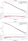 |
Fig. 1. Matter power spectrum and fractional matter power spectrum of PM simulations before and after using the HPN correction model and the theoretical halofit model for redshift z = 0.03 (upper panel) and redshift z = 0.91 (lower panel). The power spectra and ratios are represented as the means over 100 independent map realizations. The shaded regions represent the standard deviation from 100 independent DLL realizations. |
In Fig. 2 we show an example of our convergence map at z = 0.91, from pure PM simulation (first panel) and the HPN corrected simulation (second panel). The HPN model sharpens structures in the lensing field without introducing any artifacts.
 |
Fig. 2. Example of convergence maps from DLL simulations. Left panel: convergence map at source redshift z = 0.91 from DLL, PM only. Right panel: same convergence map when the HPN correction is applied. |
In the upper panel of Fig. 3, we present the angular power spectrum computed from our differentiable lensing lightcone (DLL hereafter) complemented by the HPN scheme and a conventional DLL simulation with the same resolution. Both the outputs are compared to the κTNG-Dark prediction. In the lower panel of Fig. 3 the fractional differences between the convergence power spectra from the two maps and the κTNG-Dark are shown. Both the power spectra and ratios are averaged over N = 100 realizations. We can see that the HPN model reduces the relative deviations of the angular power spectra to within 30%. We also observe a perfect match at large scales, since the κTNG-Dark and the DLL simulations have the same box size of 205 Mpc h−3.
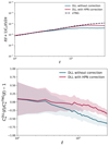 |
Fig. 3. Validation of DLL simulations against high-resolution κTNG-Dark simulations before and after using the HPN correction model. Upper panel: angular power spectra. Lower panel: fractional angular power spectra. The power spectra and ratios are means over 100 independent map realizations and the shaded regions represent the standard deviation from 100 DLL realizations. The spectra are computed for the source redshift zs = 0.91. |
4.2. IA validation
In the upper panel of Fig. 4, we present the  and
and  contributes from our DLL simulations compared to theoretical Halofit predictions (Smith et al. 2003). In the lower panel of the same figure, we show the fractional differences between the mentioned contributions. To validate the IA infusion (only for this experiment), we ran simulations while keeping the term AIA = 1. As we can see, the fractional difference for the
  term features uncertainty consistent with
  term, validating our infusion process. The signal is computed for the source redshift zs = 0.91 and is averaged over 100 realizations. The theoretical predictions are computed using the public1 Core Cosmological Library (CCL, Chisari et al. 2019).
 |
Fig. 4. Validation of the intrinsic alignment implementation in DLL simulations compared to theoretical Halofit prediction. Upper panel: |
4.3. Lensing Cℓ
To quantify the accuracy of the simulations, we aim to reproduce the summary statistics from the “dark matter only” κTNG-Dark simulations. We compare the results from the angular power spectrum for different source redshift, just by investigating how well we can recover the power spectrum for a given source plane. The results of the angular power spectrum from the sources redshift z = [0.25, 0.46, 0.65, 0.91, 1.30] are shown in the upper panel of Fig. 5, as well as the fractional differences between the κTNG-Dark and DLL maps in the lower panel. We observe that the differences for zs = 0.91 and zs = 1.30 curves are within 10% of accuracy for scales larger than ℓ = 1000, within 25% for scales 1000 < ℓ < 2000, and within 25% and 45% for scales 2000 < ℓ < 3000. For lower source redshifts, the deficit of power in our simulations becomes worse. This can be explained considering that a given value of ℓ at lower redshift corresponds to smaller scales, some of those below the resolution of our simulations. We conclude that, if for z = 0.91 and z = 1.30, we have a general agreement with κTNG-Dark; with this specific setting of the model, we cannot model cases correctly with sources redshift lower than z = 0.91.
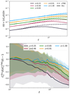 |
Fig. 5. Validation of DLL simulations for 5 source redshift against κTNG-Dark simulations. Upper panel: angular power spectra from our DLL maps compared to the κTNG-Dark predictions. Lower panel: fractional angular power spectra of DLL simulations and κTNG-Dark simulations. The power spectra mean over 100 independent map realizations and the shaded regions represent the standard deviation from 100 independent DLL realizations. |
We want to highlight that the results shown are produced keeping the resolution of the simulations extremely low, and we do not expect to get the same precision as κTNG-Dark. The purpose of these tests and the overall goal of the paper is to present a proof of concept of the DLL package and its potential. In practice, we do not work at this resolution. Nevertheless, we note that the simulations presented here already achieve a similar resolution of the MassiveNus simulations (Liu et al. 2018), despite having been generated using one single GPU.
4.4. Peak counts
We compute the starlet peak counts as wavelet coefficients with values higher than their eight neighbors. We define Jmax = 7 in Eq. (20), this starlet filter applied to our map with a pixel size of 0.29 arcmin, corresponds to a decomposition in 7 maps of resolution [0.59, 1.17, 2.34, 4.68, 9.33, 18.79, and 37.38] arcmin and a coarse map. To satisfy the survey requirement and keep the analysis centered in the range ℓ = [300, 3000], we consider only the scales corresponding to [9.33, 18.79, 37.38] arcmin. The peaks are counted for 8 linearly spaced bins within the range (κ * 𝒲) = [−0.1, 1.].
As with the power spectrum, we compare the peak counts statistic from our map to the one from the κTNG-Dark for different redshift bins. We present the results in Fig. 6. These results are shown in terms of S/N, where the signal-to-noise is defined as the ratio between the amplitude of wavelet coefficients over the noise expected for our survey choice. At a wavelet scale θ = 9.33 arcmin the differences for the zs = 0.91 curves are within the 20% up to S/N = 3; for S/N > 3 the accuracy is between the 20% and the 50%. At larger scales, θ = 18.79 arcmin the accuracy is within 20%. Finally, at θ = 37.38 arcmin the accuracy is within 15%, except for S/N < 1 where the accuracy decreases up to 28%. The results slightly improve for z = 1.30, showing an accuracy within the 35% for scale θ = 9.33 arcmin, within the 10% for θ = 18.79 arcmin and 25% for θ = 37.38 arcmin. As for the power spectrum case, we observe higher discrepancies at lower redshift; hence we can conclude that with the current setting of our simulation, we cannot correctly model such redshifts.
 |
Fig. 6. Fractional number of peaks of DLL simulations and κTNG-Dark simulations for different source redshifts. The peak counts distributions are shown for each starlet scales resolutions used: 9.34 (upper panel), 18.17 (center panel), and 37.38 arcmins (lower panel). The results mean over 100 independent map realizations and the shaded regions represent the standard deviation from 100 independent DLL realizations. |
5. Application: Fisher forecast
As an example of the application of differentiable simulations, we aim to investigate the degeneracy between the cosmological parameters in high dimensional space in cases where the systematics, such as the intrinsic alignment, is included in the analysis. Thanks to automatic differentiation, taking the derivative through the simulation with respect to the initial cosmological and nuisance parameters is now possible, thus allowing (among other things) for Fisher forecasts. In this section, we briefly introduce the Fisher forecast formalism. We also describe in detail the specific choices for the analysis we used throughout.
5.1. Forecast formalism
Fisher forecast is a widely used tool in cosmology for different purposes, for instance, to investigate the impact of systematic sources or forecast the expected constraining power of the analysis (Tegmark et al. 1997). It can be thought of as a tool to forecast error from a given experimental setup and quantify how much information we can extract from it. The Fisher matrix is defined as the expectation value of the Hessian matrix of the negative log-likelihood ℒ(C(ℓ);θ):
 (33)
(33)
where we indicate, using θ, the cosmological parameters or any systematics included in the simulation. If we assume a Gaussian likelihood and a Covariance matrix Cij independent of θ, we can calculate the Fisher matrix as
 (34)
(34)
where we use  to indicate the derivatives of the summary statistics with respect to the cosmological or nuisance parameters evaluated at the fiducial values. So, under the assumption of Gaussian likelihood, the Fisher information matrix provides a lower bound on the expected errors on cosmological parameters.
5.2. Analysis choices
To perform our study we used a single source redshift at z = 0.91. Specifically, we generated 5000 independent map realizations, to which we added Gaussian noise with mean zero and variance, as follows:
 (35)
(35)
where we set the shape noise as σe = 0.26, the pixel area as Apix = 0.086 arcmin2, and the galaxy number density as ngal = 20 arcmin−2. We assume a parameter-independent covariance matrix computed as:
 (36)
(36)
where N is the number of independent realizations,  is the value of the summary statistics in the ith bin for a given realization, r, and μ is the mean of the summary statistics over all the realization in a given bin. In addition, we adopted the estimator introduced by Hartlap et al. (2007) to take into account the loss of information caused by the finite numbers of bins and realizations, namely, we compute the inverse of the covariance matrix as:
 (37)
(37)
where C* is the covariance matrix defined in Eq. (36). As mentioned before, we want to focus on a fair comparison between the power spectrum and the peak counts method. To be sure we are considering the same scales for both statistics, we apply a wavelet pass-band filter to the maps to isolate particular scales before measuring the power spectrum. We used the same scales used for the Peak counts, namely, we decomposed the noisy convergence map in seven images, we summed up only the three maps corresponding to [9.33, 18.79, 37.38] arcmin and computed the angular Cℓ on the resulting image. An example of the Cℓ computed for each individual starlet scale image and for the summed image is depicted in Fig. 7. For each map, we computed the angular power spectrum and the peak counts by using our own differentiable code implemented in the TensorFlow framework2.
 |
Fig. 7. Example of the filtered Cℓ used for the analysis. The colored lines show the Cℓ computed on maps with a different resolution of the starlet decomposition. Specifically: the blue line (multiscale map) corresponds to Cℓ computed on the summed image; the black dashed line (Original map) corresponds to the standard Cℓ computed from a non-filtered map. |
The derivatives with respect to all parameters were evaluated at the fiducial cosmology as the mean of 1500 and 2600 independent measurements for the peak counts and Cℓ, respectively. Indeed, while the peak counts reach the convergence with ∼1500 simulations, the Cℓ proves to be more sensitive to noise and thus, requires more realizations to convergence. In Fig. B.1, we tested the stability of the Fisher contours by changing the number of simulated maps used to compute the Jacobian.
The priors used in the forecast process, are listed in Table 2 following Zhang et al. (2022). To take into account the partial coverage of the sky, we scaled the Fisher matrix by the ratio fmap/fsurvey, where fmap is the angular extend of our κmap fmap = 25 deg2 and fsurvey corresponds to the size of the convergence maps for a Stage IV-like survey fsurvey = 15 000 deg2.
Prior and fiducial values used for the forecasting.
5.3. Results
We go on to compare the relative constraining power of the two statistics described in Sect. 2.3 using the Fisher matrix formalism. As mentioned before, our interest is to investigate the sensitivity of the two weak-lensing statistics when systematics, such as the intrinsic alignment, and more cosmological parameters are included in the forecast. The results presented here are obtained from one single source redshift at z = 0.91, assuming the fiducial cosmology and survey requirement presented in Sect. 4 and Sect. 5.2. The fiducial and priors ranges of the parameters are listed in Table 2.
Figure 8 shows the 2σ contours on the full ΛCDM parameter space and intrinsic alignment term considered for the two analyses. The contours obtained by the angular Cℓ analysis are plotted in grey, and the ones for the peak counts in yellow. We find that in constraining Ωc, σ8 and AIA peak counts outperform the power spectrum, while h, ns, and Ωb parameters, within the limit of our setting, are not constrained by either and are prior dominated.
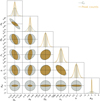 |
Fig. 8. 2σ contours derived for one single source redshift at z = 0.91 and the survey setup presented in Sect. 4. The constraints are obtained by applying the starlet Peak counts (yellow contours) computed on noisy maps filtered using a starlet kernel of [9.33, 18.70, 37.38] arcmin together and the wavelet pass-band filter for the Cℓ statistics (grey contours) as described in Sect. 4. The dashed black lines are located at the fiducial parameter values. |
This is an interesting result, confirming the higher constraining power of weak-lensing peak counts as found in Ajani et al. (2020), especially considering that the two studies differ in multiple aspects. The most important difference between these two analyses is the parameters they include. While Ajani et al. (2020) derived constraints on the sum of neutrino masses, Mν, the total matter density, Ωm, and the primordial power spectrum normalization, As, we include the five cosmological parameters of the ΛCDM model and intrinsic alignment amplitude. The constraining power of the peak count statistic keeps being higher even in high dimensional cosmological parameter space and when the intrinsic alignment is included.
The chosen angular scales differ as well. Ajani et al. (2020) considered angular scales in the range l = [300, 5000], while we focus, for both multiscale peak counts and Cℓ, on scale approximately corresponding to the range l = [300, 3000]. Despite the fact that we are neglecting scales ℓ > 3000, containing a larger amounts of non-Gaussian information, we find that for mildly nonlinear scales we are considering, the peak counts statistic still constrains the cosmological parameters the most. Finally, we find that the contours on the galaxy intrinsic alignment are significantly better constrained by the peak counts.
6. Discussion
In this section, we discuss the limitations of the methodology and results obtained in this paper, while highlighting the strategies for future extensions and applications.
In this work, we only used a single source plane in our Fisher forecast analysis, which does not allow us to evaluate the full impact that IA would have in a tomographic analysis. In particular, we do not have a contribution from the GI term. Many studies have demonstrated that the tomographic analysis can significantly improve constraints on cosmological and IA parameters (King & Schneider 2003; Heymans et al. 2004; Troxel & Ishak 2015). Although it is straightforward to generalize all the results shown in this paper to the tomographic case, this would require increasing the resolution of the simulation at lower redshifts (as illustrated by Fig. 5) in order to model correctly low redshift bins. Since the maximum number of particles we can adopt in a simulation is closely limited to the GPU memory, we are building a distributed implementation of DLL that will allow us to increase the resolutions of the simulations to the point of modeling correctly even the smaller scales at the lower redshifts. Indeed, current GPU-based simulations are capable of simulating 2563 particles on most available GPUs, and even 5123 particles on the latest h-100 NVIDIA GPUs, which come with 80 GB of memory. This capability already allows us to run realistic simulations for developing pipelines for cosmological analysis. To surpass these limitations, we are actively developing distributed implementations. It is worth noting that this has already been achieved for previous generations of simulations, such as FlowPM, which can run 20483 particles across 256 NVIDIA V100 GPUs. Additionally, we should mention that these simulations can also run on CPUs, which are less constrained by memory but lack GPU-based accelerations. A time-scaling comparison of GPU and CPU-based simulations is presented in Modi et al. (2021) and Li et al. (2022). The results clearly demonstrate the advantages of GPU-based simulations, even when not considering additional benefits such as automatic differentiation capabilities.
Another direction for further development is ray tracing methodology. In our method, we construct the weak-lensing maps assuming the Born approximation. However, Petri et al. (2017) shows that for an LSST-like survey, while the Born approximation leads to negligible parameter bias for the power spectrum, it can lead to significant parameter bias for higher order statistics. Hence, the natural next step will be to implement a ray-tracing algorithm beyond the Born approximation in our pipeline. We aim to adopt the multiple-lens-plane approximation (Blandford & Narayan 1986; Seitz et al. 1994; Jain et al. 2000; Vale & White 2003; Hilbert et al. 2009), namely, by introducing lens planes perpendicular to the line-of-sight, the deflection experienced by the light rays due to the matter inhomogeneities will be approximated through multiple deflections at the lens planes. More specifically, we will implement the memory-efficient ray-tracing scheme proposed by Hilbert et al. (2009) in the Tensorflow framework.
On the theoretical modeling side, we studied the impact of the intrinsic alignment of galaxies while assuming a linear coupling between the intrinsic galaxy shapes and the nonlinear projected tidal fields, namely, by adopting the NLA model. This physical description for the IA is only an approximation since it does not take into account the tidal torque field. In future work, we aim to extend the NLA model by implementing the extended δNLA model, described by Harnois-Déraps et al. (2022).
Finally, we have presented a tool based on only dark matter simulations. We note that this would force us to perform conservative scale cuts in the inference analysis to avoid including scales affected by baryonic effects. A future prospect is to include baryonic effects in the analysis. One possible way applicable to our methodology could be to extend the HPN ODE approach and apply more sophisticated models to learn the physics that controls the hydrodynamics simulations.
We expect that the methods illustrated in this paper will be extended to different relevant use cases. A particularly suitable example is related to the application of such algorithms as variational inference and Hamiltonian Monte Carlo, which are widely used in the Bayesian inference context and were excluded thus far due to the lack of derivatives. A further example is provided by Zeghal et al. (2022), which demonstrates that having access to the gradients of the forward model is beneficial in constraining the posterior density estimates.
7. Conclusions
In this paper, we present the Differentiable Lensing Lightcone (DLL) model, a fast lensing lightcone simulator providing access to the gradient. We extended the public FlowPM N-body code, implementing the Born approximation in the Tensorflow framework to create non-Gaussian convergence maps of weak gravitational lensing. To allow DLL to run at low resolution without affecting significantly the accuracy, we complemented the FlowPM N-body code with the HPN scheme, a new correction scheme for quasi N-body PM solver, based on neural networks implemented as a Fourier-space filter. We validate our tool by comparing the Cℓ and peak counts statistics against predictions from κTNG-Dark simulations. To do this, we ran simulations following the evolution of 1283 particles and we produced weak-lensing convergence maps for several redshift sources. We show that despite being generated at low computation costs, we recovered a good match for redshift equal to or higher than z = 0.91. To demonstrate the potential of our tool, as a first use case, we exploited the automatic differentiability of the simulations to do Fisher forecast. Thanks to back-propagation, accessing the derivative through the simulations with respect to the cosmological parameters and AIA parameter is possible at the same computational cost as the forward simulation. Assuming an LSST-like setting, we simulated weak-lensing convergence maps for a single source redshift z = 0.91 and an angular extension of 5°, based on a periodic box of comoving volume equal to 205 h−1 Mpc. We computed the constraints on the resulting convergence maps with the starlet peak counts and use a wavelet-filtered lensing power spectrum as a benchmark for the comparison. Within the limits of the analysis choices made in this study, we obtained the following results:
-
We confirm that the peak count statistics outperform the two-point statistics as found in Ajani et al. (2020), even in a high-dimensional cosmological and nuisance parameter space.
-
We find the peak counts to provide the most stringent constraints on the galaxy intrinsic alignment amplitude, AIA.
To conclude, the framework outlined here can provide many advantages in the context of cosmological parameter inference, as it marks the first step in the development of fully differentiable inference pipelines for weak lensing. Furthermore, it serves as a fast tool for further exploring the sensitivity of higher order statistics to systematics.
Code publicly available at:
https://github.com/LSSTDESC/DifferentiableHOS/tree/main/DifferentiableHOS/statistics
Acknowledgments
DESC acknowledges ongoing support from the IN2P3 (France), the STFC (United Kingdom), and the DOE, NSF, and LSST Corporation (United States). DESC uses resources of the IN2P3 Computing Center (CC-IN2P3–Lyon/Villeurbanne – France) funded by the Centre National de la Recherche Scientifique; the National Energy Research Scientific Computing Center, a DOE Office of Science User Facility supported under Contract No. DE-AC02-05CH11231; STFC DiRAC HPC Facilities, funded by UK BEIS National E-infrastructure capital grants; and the UK particle physics grid, supported by the GridPP Collaboration. This work was performed in part under DOE Contract DE-AC02-76SF00515. This work was granted access to the HPC/AI resources of IDRIS under the allocation 2022-AD011013922 made by GENCI. B.H. is supported by the AI Accelerator program of the Schmidt Futures Foundation; J.H.D. acknowledges support from an STFC Ernest Rutherford Fellowship (project reference ST/S004858/1). The presented work used computing resources provided by DESC at the National Energy Research Scientific Computing Center, a DOE Office of Science User Facility supported by the Office of Science of the US. Department of Energy under Contract No. DEAC02-05CH11231. This paper has undergone internal review in the LSST Dark Energy Science Collaboration. We thank the internal reviewers, Virginia Ajani, William Coulton, and Jia Liu for their constructive comments. Author contributions to this work are as follows: Denise Lanzieri led the analysis and the writing of the paper. François Lanusse designed the project and contributed to code and text development. Chirag Modi contributed to the PM code and text development. Benjamin Horowitz contributed to the text and made minor code developments. Joachim Harnois-Déraps contributed to the intrinsic alignment modeling, provided general advice on simulations, and contributed to the text. Jean-Luc Starck provided expertise on wavelet peak counting and higher order weak-lensing statistics.
References
- Ade, P. A., Aghanim, N., Arnaud, M., et al. 2016, A&A, 594, A13 [NASA ADS] [CrossRef] [EDP Sciences] [Google Scholar]
- Ajani, V., Peel, A., Pettorino, V., et al. 2020, Phys. Rev. D, 102, 103531 [Google Scholar]
- Ajani, V., Starck, J.-L., & Pettorino, V. 2021, A&A, 645, L11 [NASA ADS] [CrossRef] [EDP Sciences] [Google Scholar]
- Alsing, J., Wandelt, B., & Feeney, S. 2018, MNRAS, 477, 2874 [NASA ADS] [CrossRef] [Google Scholar]
- Bernardeau, F., van Waerbeke, L., & Mellier, Y. 1997, A&A, 322, 1 [NASA ADS] [Google Scholar]
- Blandford, R., & Narayan, R. 1986, ApJ, 310, 568 [Google Scholar]
- Blazek, J. A., MacCrann, N., Troxel, M. A., & Fang, X. 2019, Phys. Rev. D, 100, 103506 [NASA ADS] [CrossRef] [Google Scholar]
- Böhm, V., Feng, Y., Lee, M. E., & Dai, B. 2021, Astron. Comput., 36, 100490 [CrossRef] [Google Scholar]
- Boruah, S. S., Rozo, E., & Fiedorowicz, P. 2022, MNRAS, 516, 4111 [NASA ADS] [CrossRef] [Google Scholar]
- Boyle, A., Uhlemann, C., Friedrich, O., et al. 2021, MNRAS, 505, 2886 [NASA ADS] [CrossRef] [Google Scholar]
- Bridle, S., & King, L. 2007, New J. Phys., 9, 444 [Google Scholar]
- Brown, M., Taylor, A., Hambly, N., & Dye, S. 2002, MNRAS, 333, 501 [NASA ADS] [CrossRef] [Google Scholar]
- Campagne, J. E., Lanusse, F., Zuntz, J., et al. 2023, Open J. Astrophys., 6 [Google Scholar]
- Catelan, P., Kamionkowski, M., & Blandford, R. D. 2001, MNRAS, 320, L7 [NASA ADS] [CrossRef] [Google Scholar]
- Chen, R. T., Rubanova, Y., Bettencourt, J., & Duvenaud, D. K. 2018, Adv. Neural Inf. Process. Syst., 31 [Google Scholar]
- Cheng, S., & Ménard, B. 2021, MNRAS, 507, 1012 [NASA ADS] [CrossRef] [Google Scholar]
- Chisari, N. E., Alonso, D., Krause, E., et al. 2019, ApJS, 242, 2 [Google Scholar]
- Eisenstein, D. J., & Hu, W. 1998, ApJ, 496, 605 [Google Scholar]
- Feng, Y., Chu, M. Y., Seljak, U., & McDonald, P. 2019, Astrophysics Source Code Library [record ascl:1905.010] [Google Scholar]
- Fluri, J., Kacprzak, T., Lucchi, A., et al. 2019, Phys. Rev. D, 100, 063514 [Google Scholar]
- Fluri, J., Kacprzak, T., Refregier, A., Lucchi, A., & Hofmann, T. 2021, Phys. Rev. D, 104, 123526 [NASA ADS] [CrossRef] [Google Scholar]
- Fluri, J., Kacprzak, T., Lucchi, A., et al. 2022, Phys. Rev. D, 105, 083518 [NASA ADS] [CrossRef] [Google Scholar]
- Gatti, M., Jain, B., Chang, C., et al. 2022, Phys. Rev. D, 106, 083509 [NASA ADS] [CrossRef] [Google Scholar]
- Halder, A., Friedrich, O., Seitz, S., & Varga, T. N. 2021, MNRAS, 506, 2780 [CrossRef] [Google Scholar]
- Harnois-Déraps, J., Martinet, N., & Reischke, R. 2022, MNRAS, 509, 3868 [Google Scholar]
- Hartlap, J., Simon, P., & Schneider, P. 2007, A&A, 464, 399 [NASA ADS] [CrossRef] [EDP Sciences] [Google Scholar]
- Heymans, C., Brown, M., Heavens, A., et al. 2004, MNRAS, 347, 895 [Google Scholar]
- Hilbert, S., Hartlap, J., White, S. D. M., & Schneider, P. 2009, A&A, 499, 31 [NASA ADS] [CrossRef] [EDP Sciences] [Google Scholar]
- Hirata, C. M., & Seljak, U. 2004, Phys. Rev. D, 70, 063526 [Google Scholar]
- Hockney, R., & Eastwood, J. 1988, Computer Simulation Using Particles (USA: Taylor& Francis, Inc.) [CrossRef] [Google Scholar]
- Ivezić, Ž., Kahn, S. M., Tyson, J. A., et al. 2019, ApJ, 873, 111 [Google Scholar]
- Jain, B., & Seljak, U. 1997, ApJ, 484, 560 [Google Scholar]
- Jain, B., Seljak, U., & White, S. 2000, ApJ, 530, 547 [NASA ADS] [CrossRef] [Google Scholar]
- Jeffrey, N., Alsing, J., & Lanusse, F. 2021, MNRAS, 501, 954 [Google Scholar]
- Kacprzak, T., & Fluri, J. 2022, Phys. Rev. X, 12, 031029 [NASA ADS] [Google Scholar]
- Kacprzak, T., Kirk, D., Friedrich, O., et al. 2016, MNRAS, 463, 3653 [Google Scholar]
- Kilbinger, M. 2015, Rep. Prog. Phys., 78, 086901 [Google Scholar]
- King, L. J., & Schneider, P. 2003, A&A, 398, 23 [NASA ADS] [CrossRef] [EDP Sciences] [Google Scholar]
- Kratochvil, J. M., Lim, E. A., Wang, S., et al. 2012, Phys. Rev. D, 85, 103513 [Google Scholar]
- Lanzieri, D., Lanusse, F., & Starck, J. L. 2022, Machine Learning for Astrophysics, proceedings of the Thirty-ninth International Conference on Machine Learning (ICML 2022), July 22nd, Baltimore, MD, online at https://ml4astro.github.io/icml2022, 60 [Google Scholar]
- Laureijs, R., Amiaux, J., Arduini, S., et al. 2011, ArXiv e-prints [arXiv:1110.3193] [Google Scholar]
- Li, Y., Modi, C., Jamieson, D., et al. 2022, ArXiv e-prints [arXiv:2211.09815] [Google Scholar]
- Lin, C.-A., & Kilbinger, M. 2015, A&A, 583, A70 [NASA ADS] [CrossRef] [EDP Sciences] [Google Scholar]
- Lin, C.-A., Kilbinger, M., & Pires, S. 2016, A&A, 593, A88 [NASA ADS] [CrossRef] [EDP Sciences] [Google Scholar]
- Liu, J., & Madhavacheril, M. S. 2019, Phys. Rev. D, 99, 083508 [Google Scholar]
- Liu, J., Petri, A., Haiman, Z., et al. 2015a, Phys. Rev. D, 91, 063507 [Google Scholar]
- Liu, X., Pan, C., Li, R., et al. 2015b, MNRAS, 450, 2888 [Google Scholar]
- Liu, J., Bird, S., Matilla, J. M. Z., et al. 2018, JCAP, 2018, 049 [CrossRef] [Google Scholar]
- Makinen, T. L., Charnock, T., Alsing, J., & Wandelt, B. D. 2021, JCAP, 2021, 049 [CrossRef] [Google Scholar]
- Mandelbaum, R., Eifler, T., Hložek, R., et al. 2018, ArXiv e-prints [arXiv:1809.01669] [Google Scholar]
- Martinet, N., Schneider, P., Hildebrandt, H., et al. 2018, MNRAS, 474, 712 [Google Scholar]
- Modi, C., Lanusse, F., & Seljak, U. 2021, Astron. Comput., 37, 100505 [NASA ADS] [CrossRef] [Google Scholar]
- Osato, K., Liu, J., & Haiman, Z. 2021, MNRAS, 502, 5593 [Google Scholar]
- Peel, A., Lin, C.-A., Lanusse, F., et al. 2017, A&A, 599, A79 [NASA ADS] [CrossRef] [EDP Sciences] [Google Scholar]
- Petri, A., Haiman, Z., Hui, L., May, M., & Kratochvil, J. M. 2013, Phys. Rev. D, 88, 123002 [Google Scholar]
- Petri, A., Haiman, Z., & May, M. 2017, Phys. Rev. D, 95, 123503 [NASA ADS] [CrossRef] [Google Scholar]
- Pontryagin, L., Boltyanski, V., Gamkrelidze, R., & Mishchenko, E. 1962, The Mathematical Theory of Optimal Processes (New York: Interscience) [Google Scholar]
- Porqueres, N., Heavens, A., Mortlock, D., & Lavaux, G. 2021, MNRAS, 502, 3035 [NASA ADS] [CrossRef] [Google Scholar]
- Rizzato, M., Benabed, K., Bernardeau, F., & Lacasa, F. 2019, MNRAS, 490, 4688 [NASA ADS] [CrossRef] [Google Scholar]
- Schneider, P. 2006, Gravitational Lensing: Strong, Weak and Micro (Springer), 269 [NASA ADS] [CrossRef] [Google Scholar]
- Schneider, P., & Lombardi, M. 2003, A&A, 397, 809 [NASA ADS] [CrossRef] [EDP Sciences] [Google Scholar]
- Seitz, S., Schneider, P., & Ehlers, J. 1994, CQG, 11, 2345 [NASA ADS] [CrossRef] [Google Scholar]
- Semboloni, E., Schrabback, T., van Waerbeke, L., et al. 2011, MNRAS, 410, 143 [Google Scholar]
- Shan, H., Liu, X., Hildebrandt, H., et al. 2018, MNRAS, 474, 1116 [Google Scholar]
- Smith, R. E., Peacock, J. A., Jenkins, A., et al. 2003, MNRAS, 341, 1311 [Google Scholar]
- Spergel, D., Gehrels, N., Baltay, C., et al. 2015, ArXiv e-prints [arXiv:1503.03757] [Google Scholar]
- Springel, V. 2010, MNRAS, 401, 791 [Google Scholar]
- Starck, J.-L., Fadili, J., & Murtagh, F. 2007, IEEE Trans. Image Process., 16, 297 [Google Scholar]
- Starck, J.-L., Murtagh, F., & Fadili, J. 2010, Sparse Image and Signal Processing: Wavelets, Curvelets, Morphological Diversity (USA: Cambridge University Press) [CrossRef] [Google Scholar]
- Takada, M., & Jain, B. 2004, MNRAS, 348, 897 [Google Scholar]
- Takahashi, R., Sato, M., Nishimichi, T., Taruya, A., & Oguri, M. 2012, ApJ, 761, 152 [Google Scholar]
- Tegmark, M., Taylor, A. N., & Heavens, A. F. 1997, ApJ, 480, 22 [NASA ADS] [CrossRef] [Google Scholar]
- Troxel, M., & Ishak, M. 2015, Phys. Rep., 558, 1 [NASA ADS] [CrossRef] [Google Scholar]
- Uhlemann, C., Friedrich, O., Villaescusa-Navarro, F., Banerjee, A., & Codis, S. 2020, MNRAS, 495, 4006 [NASA ADS] [CrossRef] [Google Scholar]
- Vale, C., & White, M. 2003, ApJ, 592, 699 [CrossRef] [Google Scholar]
- van Waerbeke, L., Bernardeau, F., & Mellier, Y. 1999, A&A, 342, 15 [NASA ADS] [Google Scholar]
- Villaescusa-Navarro, F., Anglés-Alcázar, D., Genel, S., et al. 2021, ApJ, 915, 71 [NASA ADS] [CrossRef] [Google Scholar]
- Zeghal, J., Lanusse, F., Boucaud, A., Remy, B., & Aubourg, E. 2022, Machine Learning for Astrophysics, proceedings of the Thirty-ninth International Conference on Machine Learning (ICML 2022), July 22nd, Baltimore, MD, online at https://ml4astro.github.io/icml2022, 52 [Google Scholar]
- Zhang, Z., Chang, C., Larsen, P., et al. 2022, MNRAS, 514, 2181 [NASA ADS] [CrossRef] [Google Scholar]
- Zürcher, D., Fluri, J., Sgier, R., et al. 2022, MNRAS, 511, 2075 [CrossRef] [Google Scholar]
Appendix A: Validation against a theory prediction
We show the 2σ constraints obtained from our Fisher analysis of standard Cℓ (orange) and the theoretical prediction from halofit (blue contours) in Figure A.1. The dashed black contours define the prior used for the forecasting. The analysis is performed for one single source redshift at z = 0.91 and the survey setup presented in Section 4.
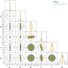 |
Fig. A.1. 2σ contours derived for one single source redshift at z = 0.91 and the survey setup presented in Section 4. We compare the Fisher matrix constraints on cosmological parameters and AIA amplitude obtained with the Cℓ from our mock maps (orange) and the theoretical Cℓ (blue) obtained from the public library https://github.com/DifferentiableUniverseInitiative/jaxcosmo (Campagne et al. 2023). In both cases, the constraints are obtained by applying the wavelet pass-band filter for the Cℓ as described in Section 4. The dashed black contours are the prior used for the forecasting. |
The constraints from the theoretical predictions are compatible with the ones obtained from the mock DLL maps for all cosmological parameters, except ns. Indeed, despite sharing the same direction of the degeneracy, the theoretical contours for ns are narrower compared to the ones obtained in our analysis. In general, this translates into an increased uncertainty in constraining ns, most likely due to the deficit in power observed for the Cℓ at small scales.
The theoretical predictions are computed using the public library jax-cosmo (Campagne et al. 2023). We want to highlight that both the theoretical Fisher matrices and the ones from our analysis are obtained by automatic differentiation.
Appendix B: Validation of the stability of the Fisher contours
To ensure that the shape of the ellipses and the direction of the degeneracies are not the results of stochasticity, we prove the stability of the Fisher analysis results by testing the convergence of the Jacobians. In Figure B.1 we present the results for Fisher constraints obtained when varying the number of independent simulations used to compute the Jacobians. As we can see, the convergence seems to be reached for the peak counts with, at least, 1500 realizations. On the other hand, the angular Cℓ proves to be more sensitive to noise and thus requires at least 2600 realizations.
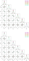 |
Fig. B.1. 1σ Fisher contours derived for one single source redshift at z = 0.91 and the survey setup presented in Section 4 for the Cℓ (upper panel) and the Peak counts (lower panel). The different colors refer to the number of independent realizations used to mean the Jacobian in the Equation 34. The dashed black lines are located at the fiducial parameter values. |
Appendix C: Validation with higher resolutions simulations
In Section 4, we presented a validation of our simulations by comparing the statistics from DLL and κTNG-Dark. In particular, we have seen a discrepancy on small scales for both the Cℓ and the peak counts. We have attributed this bias to the low resolution of the simulations. Therefore, to justify this assumption, we simulated convergence maps of higher resolution; namely, we raised the number of particles but keep the same box of 2053(h−1Mpc)3 in the simulation. In the left panel of Figure C.1, we present the angular power spectrum computed from our DLL with the original number count of particles (1283) and the power spectrum computed from higher resolutions DLL simulations (2123). The two outputs are compared to the κTNG-Dark predictions. In the right panel of Figure C.1 the fractional differences between the convergence power spectra from the two maps and the κTNG-Dark are shown. We can see that by increasing the number of particles, we can improve the accuracy of the lensing Cℓ up to 20%. In Figure C.2, we compare the peak counts statistic from our map to the one from the κTNG-Dark for different resolutions. We use the same wavelet decomposition presented in Section 4.4. As for the power spectrum, we note the same tendency to recover better accuracy when the resolution is increased.
 |
Fig. C.1. Comparison of DLL simulations with original (number count 1283) and higher resolutions (number count 2123) against high-resolution κTNG-Dark simulations. Left panel: Angular power spectra of PM simulations with original resolution (blue line) and higher resolution (red line) compared to the κTNG-Dark prediction. Right panel: fractional angular power spectrum of PM simulations with original and higher resolution and the κTNG-Dark prediction. The power spectra and ratios are means over 100 independent map realizations and the shaded regions represent the error on the mean. The spectra are computed for the source redshift zs = 0.91. |
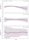 |
Fig. C.2. Fractional number of peaks of DLL simulations and κTNG-Dark simulations. The results are shown for the number counts 1283 (blue lines) and 2123 (orange lines). The peak count distributions are shown for each starlet scale resolution used: 9.34 (upper panel), 18.17 (center panel), and 37.38 arcmins (lower panel). The results show the mean over 100 independent map realizations, the shaded regions represent the error on the mean. The statistics are computed for the source redshift of zs = 0.91. |
Finally, we reproduce the results of the Fisher analysis for the intrinsic alignment parameter AIA with higher-resolution simulations in Figure C.3. We adopted the same Forecast criteria presented in Section 5. However, for this specific test, we compute the derivatives numerically using the finite differences. The step sizes used for these variations are ΔxIA = 0.15 for the Cℓ and ΔxIA = 1.2 for the peak counts. In order to check the reliability of the numerical derivatives, we investigate the stability of the Fisher forecast against different step sizes used to compute them. The derivatives are computed as the mean of 3000 independent realizations for both Cℓ and peak counts.
 |
Fig. C.3. 1σ error on AIA for one single source redshift at z = 0.91 and the survey setup presented in Section 4, from mock simulations with 2123 particles. The results are obtained by applying the starlet Peak counts (yellow contours) computed on noisy maps filtered using a starlet kernel of [9.33, 18.70, 37.38] arcmin together and the wavelet pass-band filter for the Cℓ statistics (grey contours) as described in Section 4. |
We confirmed the peak counts provide the most stringent constraints on the galaxy intrinsic alignment amplitude AIA. As for the full analysis, we tested the stability of the Fisher forecast by varying the number of simulated maps used to compute the derivatives. In Figure C.4 we present the 1σ error on AIA when varying the number of independent realizations used to compute the derivatives. It is interesting to note that even in this case, the derivatives of the Cℓ can not be considered fully converged. However, as can be noted from the stability plots of Figure C.4, the noise in the derivatives leads to tighter constraints in the Fisher forecast. Hence, the fully converged derivatives of the Cℓ would result in even broader constraints, without changing the results we found.
 |
Fig. C.4. 1σ error on AIA derived for one single source redshift at z = 0.91 for different numbers of independent realizations used to mean the Jacobian in the Equation 34. The results are shown for the Cℓ (left panel) and the peak counts (right panel). |
All Tables
All Figures
 |
Fig. 1. Matter power spectrum and fractional matter power spectrum of PM simulations before and after using the HPN correction model and the theoretical halofit model for redshift z = 0.03 (upper panel) and redshift z = 0.91 (lower panel). The power spectra and ratios are represented as the means over 100 independent map realizations. The shaded regions represent the standard deviation from 100 independent DLL realizations. |
| In the text | |
 |
Fig. 2. Example of convergence maps from DLL simulations. Left panel: convergence map at source redshift z = 0.91 from DLL, PM only. Right panel: same convergence map when the HPN correction is applied. |
| In the text | |
 |
Fig. 3. Validation of DLL simulations against high-resolution κTNG-Dark simulations before and after using the HPN correction model. Upper panel: angular power spectra. Lower panel: fractional angular power spectra. The power spectra and ratios are means over 100 independent map realizations and the shaded regions represent the standard deviation from 100 DLL realizations. The spectra are computed for the source redshift zs = 0.91. |
| In the text | |
 |
Fig. 4. Validation of the intrinsic alignment implementation in DLL simulations compared to theoretical Halofit prediction. Upper panel: |
| In the text | |
 |
Fig. 5. Validation of DLL simulations for 5 source redshift against κTNG-Dark simulations. Upper panel: angular power spectra from our DLL maps compared to the κTNG-Dark predictions. Lower panel: fractional angular power spectra of DLL simulations and κTNG-Dark simulations. The power spectra mean over 100 independent map realizations and the shaded regions represent the standard deviation from 100 independent DLL realizations. |
| In the text | |
 |
Fig. 6. Fractional number of peaks of DLL simulations and κTNG-Dark simulations for different source redshifts. The peak counts distributions are shown for each starlet scales resolutions used: 9.34 (upper panel), 18.17 (center panel), and 37.38 arcmins (lower panel). The results mean over 100 independent map realizations and the shaded regions represent the standard deviation from 100 independent DLL realizations. |
| In the text | |
 |
Fig. 7. Example of the filtered Cℓ used for the analysis. The colored lines show the Cℓ computed on maps with a different resolution of the starlet decomposition. Specifically: the blue line (multiscale map) corresponds to Cℓ computed on the summed image; the black dashed line (Original map) corresponds to the standard Cℓ computed from a non-filtered map. |
| In the text | |
 |
Fig. 8. 2σ contours derived for one single source redshift at z = 0.91 and the survey setup presented in Sect. 4. The constraints are obtained by applying the starlet Peak counts (yellow contours) computed on noisy maps filtered using a starlet kernel of [9.33, 18.70, 37.38] arcmin together and the wavelet pass-band filter for the Cℓ statistics (grey contours) as described in Sect. 4. The dashed black lines are located at the fiducial parameter values. |
| In the text | |
 |
Fig. A.1. 2σ contours derived for one single source redshift at z = 0.91 and the survey setup presented in Section 4. We compare the Fisher matrix constraints on cosmological parameters and AIA amplitude obtained with the Cℓ from our mock maps (orange) and the theoretical Cℓ (blue) obtained from the public library https://github.com/DifferentiableUniverseInitiative/jaxcosmo (Campagne et al. 2023). In both cases, the constraints are obtained by applying the wavelet pass-band filter for the Cℓ as described in Section 4. The dashed black contours are the prior used for the forecasting. |
| In the text | |
 |
Fig. B.1. 1σ Fisher contours derived for one single source redshift at z = 0.91 and the survey setup presented in Section 4 for the Cℓ (upper panel) and the Peak counts (lower panel). The different colors refer to the number of independent realizations used to mean the Jacobian in the Equation 34. The dashed black lines are located at the fiducial parameter values. |
| In the text | |
 |
Fig. C.1. Comparison of DLL simulations with original (number count 1283) and higher resolutions (number count 2123) against high-resolution κTNG-Dark simulations. Left panel: Angular power spectra of PM simulations with original resolution (blue line) and higher resolution (red line) compared to the κTNG-Dark prediction. Right panel: fractional angular power spectrum of PM simulations with original and higher resolution and the κTNG-Dark prediction. The power spectra and ratios are means over 100 independent map realizations and the shaded regions represent the error on the mean. The spectra are computed for the source redshift zs = 0.91. |
| In the text | |
 |
Fig. C.2. Fractional number of peaks of DLL simulations and κTNG-Dark simulations. The results are shown for the number counts 1283 (blue lines) and 2123 (orange lines). The peak count distributions are shown for each starlet scale resolution used: 9.34 (upper panel), 18.17 (center panel), and 37.38 arcmins (lower panel). The results show the mean over 100 independent map realizations, the shaded regions represent the error on the mean. The statistics are computed for the source redshift of zs = 0.91. |
| In the text | |
 |
Fig. C.3. 1σ error on AIA for one single source redshift at z = 0.91 and the survey setup presented in Section 4, from mock simulations with 2123 particles. The results are obtained by applying the starlet Peak counts (yellow contours) computed on noisy maps filtered using a starlet kernel of [9.33, 18.70, 37.38] arcmin together and the wavelet pass-band filter for the Cℓ statistics (grey contours) as described in Section 4. |
| In the text | |
 |
Fig. C.4. 1σ error on AIA derived for one single source redshift at z = 0.91 for different numbers of independent realizations used to mean the Jacobian in the Equation 34. The results are shown for the Cℓ (left panel) and the peak counts (right panel). |
| In the text | |
Current usage metrics show cumulative count of Article Views (full-text article views including HTML views, PDF and ePub downloads, according to the available data) and Abstracts Views on Vision4Press platform.
Data correspond to usage on the plateform after 2015. The current usage metrics is available 48-96 hours after online publication and is updated daily on week days.
Initial download of the metrics may take a while.


