| Issue |
A&A
Volume 691, November 2024
|
|
|---|---|---|
| Article Number | A219 | |
| Number of page(s) | 18 | |
| Section | Extragalactic astronomy | |
| DOI | https://doi.org/10.1051/0004-6361/202348164 | |
| Published online | 15 November 2024 | |
Spectral reconstruction for radiation hydrodynamic simulations of galaxy evolution
1
Institute of Theoretical Astrophysics, University of Oslo, PO Box 1029 Blindern, 0315 Oslo, Norway
2
Department of Physics and Astronomy, McMaster University, Hamilton L8S 4M1, Canada
⋆ Corresponding author; This email address is being protected from spambots. You need JavaScript enabled to view it.
Received:
5
October
2023
Accepted:
12
September
2024
Abstract
Radiation from stars and active galactic nuclei (AGN) plays an important role in galaxy formation and evolution, and profoundly transforms the intergalactic, circumgalactic, and interstellar medium (IGM, CGM, and ISM). On-the-fly radiative transfer (RT) has started being incorporated in cosmological simulations, but the complex evolving radiation spectra are often crudely approximated with a small number of broad bands with piece-wise constant intensity and a fixed photo-ionisation cross-section. Such a treatment is unable to capture the changes to the spectrum as light is absorbed while it propagates through a medium with non-zero opacity. This can lead to large errors in photo-ionisation and heating rates. In this work we present a novel approach of discretising the radiation field at discrete photon energies, at the edges of the typically used photo-ionising bands, in order to capture the power-law slope of the radiation field. In combination with power-law approximations for the photo-ionisation cross-sections, this model allows us to self-consistently combine radiation from sources with different spectra and accurately follow the ionisation states of primordial and metal species through time. The method is implemented in GASOLINE2 in connection with TREVR2, a fast reverse ray tracing algorithm with 𝒪(Nactive log2 N) scaling. We compare our new piece-wise power-law reconstruction to the piece-wise constant method in calculating the primordial chemistry photo-ionisation and heating rates under an evolving UV background (UVB) and stellar spectrum, and find that our method reduces errors significantly, by up to two orders of magnitude in the case of HeII ionisation. We apply our new spectral reconstruction method in RT post-processing of a cosmological zoom-in simulation, MUGS2 g1536, including radiation from stars and a live UVB, and find a significant increase in total neutral hydrogen (HI) mass in the ISM and the CGM due to shielding of the UVB and a low escape fraction of the stellar radiation. This demonstrates the importance of RT and an accurate spectral approximation in simulating the CGM-galaxy ecosystem.
Key words: radiative transfer / methods: numerical / galaxies: evolution / galaxies: formation / galaxies: ISM
© The Authors 2024
 Open Access article, published by EDP Sciences, under the terms of the Creative Commons Attribution License (https://creativecommons.org/licenses/by/4.0), which permits unrestricted use, distribution, and reproduction in any medium, provided the original work is properly cited.
This article is published in open access under the Subscribe to Open model. This email address is being protected from spambots. You need JavaScript enabled to view it. to support open access publication.
1. Introduction
Radiation from stars and active galactic nuclei (AGN) plays an important role in galaxy formation and evolution. It can transfer momentum to gas close to sources, on scales that are typically not resolved in simulations of galaxy evolution, but radiation, in particular UV and X-ray, also affects the thermo-chemistry of gas via photo-ionisation and heating over a large range of galactic and cosmological scales (e.g. Tielens 2005; Wolfire et al. 2003; Puchwein et al. 2019).
In principle, light emitted from each source (Nsrc) has to reach each receiving gas resolution element (Nrec) in the simulation volume. Each beam of light interacts with the medium along its path, which is typically resolved by  elements. In simulations of galaxy formation, the number of sources can become comparable to the number of receiving gas elements resulting in an overall operation count of such a naive approach to be
  or 𝒪(N7/3), when Nrec = Nsrc. As the interaction of light with gas (e.g. absorption or scattering) is frequency dependent, the above operation count further depends linearly on the considered spectral resolution (i.e. the number of frequency bins Nν used in the simulation). Leong et al. (2023) found that 20 to 200 frequency bins above 13.6 eV are needed to ensure an accuracy of a few percent in the frequency integration of photo-ionisation and heating rates. Such scaling would be unfavourable for full-scale radiative transfer (RT) simulations, so brute force approaches that scale as 𝒪(N7/3) are not practical and were never adopted in cosmological galaxy formation simulations. Instead, a variety of methods have been developed over the past decades to significantly improve the scaling of the RT problem, and these can be loosely classified into evolutionary and instantaneous methods.
Evolutionary methods advect radiation energy throughout the simulation. They include moment-based methods, which solve for moments of the radiation transport equations, and thus the radiation field is propagated on the grid and is solved in a similar fashion to the equations of hydrodynamic. Examples are flux-limited diffusion (Levermore & Pomraning 1981), the Optically Thin Variable Eddington Tensor (OTVET) approximation (Gnedin & Abel 2001), and the M1-closure (González et al. 2007) as applied in RAMSES-RT (Rosdahl et al. 2013) and AREPO-RT (Kannan et al. 2019). These methods scale as 𝒪(N) and are independent of the number of sources, as their emission is mapped onto the grid with N resolution elements. However, a short time-step is required (though the speed of light is often reduced to speed up the code, Rosdahl et al. 2015). Cells must be evaluated, either at every step or with an adaptive time-step that performs detailed bookkeeping to conserve photons (e.g. Kannan et al. 2019).
Instantaneous methods are typically ray tracing methods that solve the RT problem along rays cast either from the sources to the receiver (forward ray tracing) or with rays built in the opposite direction (reverse ray tracing). In ray tracing, 𝒪(N2/3) rays are sufficient to pass close to every absorber, and thus the scaling is usually no worse than 𝒪(N2). Reverse ray tracing algorithms, such as TREERAY (Wünsch et al. 2018) or TREVR/TREVR2 (Grond et al. 2019; Wadsley et al. 2024) approximate distant sources by combining them within tree nodes, reducing the effective number of sources to log2(Nsrc). This gives an overall 𝒪(N log2(N)) scaling. In principle, the radiation field can be calculated instantaneously when needed, rather than stored.
In order to further reduce the computation time of RT calculations, the source spectrum is often approximated by a few radiation bands. RT simulations of galaxy formation need to approximate the ionising source spectrum. For photon energies above 13.6 eV, this commonly requires at least three radiation bands, namely the HI (13.6−24.6 eV), HeI (24.6−54.4 eV), and HeII (54.4–∞)1 ionising bands (e.g. Pawlik et al. 2013; Rosdahl et al. 2015; Kannan et al. 2022). A common approach is to represent each band using a constant effective photon energy with a fixed photo-ionisation cross-section. Throughout this work we refer to this spectral approximation as the piece-wise constant (PWC) approximation. The number of bands and the band boundaries are not necessarily the same between individual simulations. For example, in RAMSES-RTZ (Katz 2022), the HI ionising band is split into two bands at 15.2 eV, to separate the photo-ionisation of H2 and HI. Pallottini et al. (2022) used three narrower bands in the typical HI ionising band (13.6−24.6 eV), but only assumed collisional ionisation for He.
A low-resolution representation of the source spectrum, in combination with a fixed representative photon energy per band, can be problematic for varied sources (e.g. in age or type) and for different absorbing columns which further modify the spectra. Spectra of different shapes result in different typical photon energies, affecting both heating and the photo-ionisation cross-sections. In principle, the effective cross-section, and thus the heating and ionisation rates, need to be calculated for each gas particle based on the spectral shape it receives. In practice, it is often assumed that the source spectrum can be represented by the spectrum of a star-forming galaxy that has experienced continuous star formation over a few million years (e.g. Rosdahl et al. 2015; Pallottini et al. 2022; Kannan et al. 2022). Rosdahl et al. (2018) argued that even though radiation spectral shapes change significantly (e.g. with stellar age and metallicity), key parameters such as cross-section change in a more limited way.
This approach is likely sufficient when modelling the UV ionising radiation in the interstellar medium (ISM) of star-forming galaxies, as it is dominated by young stellar populations. However, in RT simulations with a large population of galaxies and AGN, a fixed-shape spectrum of a star-forming galaxy does not accurately represent radiation from AGN, or quiescent galaxies with older stellar populations. Moreover, as radiation propagates through a optically thick medium, frequency dependent cross-sections result in stronger absorption at lower photon energies within each radiation band (spectral hardening). It is challenging for the PWC approximation to follow spectral hardening within a radiation band. In particular, a single cross-section cannot be accurate across a range of optical depths.
These issues are important when modelling the cosmological UV background (UVB) in full radiative transfer simulations. For RT simulations of large cosmological volumes to study the epoch of reionisation (e.g. Aubert & Teyssier 2010; Shapiro et al. 2012; Gnedin 2014; Rosdahl et al. 2018; Kannan et al. 2022; Lewis et al. 2022), the ionisation background radiation is computed directly from the light emitted by stars and AGN within the simulation volume, through the use of periodic boundary conditions. If sources with different spectral shapes are included in a simulation the photo-ionisation cross-sections are often calculated assuming a fixed spectrum (e.g. Jeon et al. 2014; Kannan et al. 2022). For zoom-in simulations that focus on the ISM of the simulated galaxy, it is common that the UVB is not included (e.g. Pawlik et al. 2013; Kimm et al. 2017; Garcia et al. 2023) or included in a simplified fashion (e.g. Pallottini et al. 2019, 2022; Agertz et al. 2020; Blaizot et al. 2023), similar to what is used in simulations without RT.
A more accurate approach to tackle the multi-frequency RT problem is the two-field ansatz first developed in Gnedin & Abel (2001), in which the total radiation field is split into a mean intensity field (the UVB or diffuse sources) and a local perturbation (radiation from nearby stars). In this case, the two fields can have different spectral shapes, but the shapes are assumed independent of location and time. This makes it easy to pre-calculate the ionisation and heating rates before performing the RT and hydro steps. The assumption of fixed shapes can be further improved by taking the absorbing column into account as an extra dimension for the table. This approach is used in Gnedin (2014) and also in several zoom-in simulations (e.g. Ricotti et al. 2002; Zemp et al. 2012; Muratov et al. 2013).
An accurate multi-frequency treatment of the UVB is needed for studies of the circumgalactic medium (CGM) and galaxy co-evolution. Firstly, the CGM is highly multiphase with a wide range of densities, ionisation states, and metallicities (e.g. Tumlinson et al. 2017; Fielding et al. 2020; Decataldo et al. 2024). As such, radiation transport, both for stellar/AGN radiation outwards and for background radiation inwards, is likely to be complex. Moreover, metals in the CGM are crucial for gas cooling and subsequently impact gas dynamics and galaxy formation. However, the ionisation states of metal ions strongly depend on the radiation field, not only the intensity, but also the spectral shape. For example, one of the major coolants is the fifth ionised oxygen (OVI), which is observed to be abundant in the CGM of star-forming galaxies (e.g. Tumlinson et al. 2013; Werk et al. 2016). The ionisation potential of OVI is much higher than that of neutral hydrogen, and therefore hard photons from both the UVB and the stellar/AGN radiation are essential (e.g. Oppenheimer et al. 2018). We note that the ISM is generally more transparent to higher energy photons, and the contribution from internal radiation in the CGM closer to galaxies can be significant. While it is common for non-RT (and even RT) simulations to include tabulated metal cooling rates as a function of redshift to capture the evolving uniform UVB (e.g. Wiersma et al. 2009; Shen et al. 2010; Smith et al. 2017), such an approach fails to take into account internal radiation from galaxies and the changing spectral shape. Last but not least, observations of the CGM, both in absorption and emission, rely on certain ion tracers (e.g. Lyα, CII, CIV, OVI, MgII). An accurate modelling of the radiation field is fundamental for the interpretation of observational data.
In this work we focus on the challenges of modelling the variation of spectra from multiple radiation sources and present a novel approach to discretise the source spectra, which allows us to self-consistently combine arbitrary spectral shapes and simultaneously follow spectral hardening within the typical radiation bands naturally. The paper is structured as follows. In Sect. 2 we present our new approach to reconstruct the spectrum of the incident radiation field during hydrodynamic simulations of galaxy evolution employing on-the-fly RT. In Sect. 3 we compare our new treatment of the radiation field to commonly used simplifications based on theoretical calculations of photo-ionisation, heating rates, and simple test problems, and discuss their impact on simulations of galaxies. We show the results obtained by RT post-processing of a cosmological zoom-in simulation of galaxy evolution with our new spectral reconstruction method in Sect. 4. A final discussion is provided in Sect. 5.
2. Spectral reconstruction
The primary goal of any simulation employing far-UV radiative transfer is to self-consistently account for the interplay of matter with these high-energy photons. Among those effects are photo-electric heating of dust, photo-dissociation of molecular hydrogen, photo-ionisation, and heating of H and He. The photo-ionisation rate of a specific ion, i can be calculated by
 (1)
(1)
where Jν is the radiation field in erg cm−2 s−1 Hz−1 sr−1, h is Planck’s constant, and σi(ν) is the frequency dependent ionisation cross-section of species i. The photo-heating rate is given by
 (2)
(2)
where h ν0, i is the ionisation potential of species i. In the most general case the spectral shape of the incident radiation field Jν has a complex dependency on space, time, type of emitting sources and the intervening matter between the emitting source and receiving gas. If the spectral shape of the incident radiation and gas optical depths have strong spatial and temporal variations, naively Eqs. (1) and (2) need to be integrated numerically on-the-fly. However, in practice assumptions are often made regarding the spectral shape and spatial and/or time variability so that the ionisation and heating rates can be calculated with sufficient accuracy. For example, the source spectra can be parametrised in terms of a linear combination of a set of pre-defined spectra and the intervening absorbing column (Gnedin & Abel 2001), which allows the photo-ionisation rates to be pre-tabulated.
The spectral reconstruction method presented here seeks to simultaneously allow for the combination of different types of radiative sources with varying spectra, calculate spatially varying opacities for the radiation bands, follow spectral hardening within the classic broad ionisation bands, and be analytically integrable so that photo-ionisation and heating rates can be calculated self-consistently on-the-fly in RT simulations. It thus has similar goals to the tabulation approach, especially in terms of avoiding run-time costs. In the following section we describe our new discretisation scheme of the photo-ionisation cross-sections and the radiation field, to which we refer to as piece-wise power-law (PWPL) approximation.
2.1. Photo-ionisation cross-sections
For the PWC approximation, it is commonly assumed that the source spectrum can be represented by a unique and often time independent spectrum. Considering only the total number of photons in these bands and assuming all sources follow the same spectral shape allows for the pre-calculation of effective photo-ionisation cross-sections ( ) for each species i per ionisation band j as
 (3)
(3)
where the integration is performed over the energy limits of the considered band. The effective cross-section is then incorporating the shape information of the source spectrum. The PWC approach allows Eq. (1) to be greatly simplified, for a species i, which can be expressed as
 (4)
(4)
where  is the photon flux in photons cm−2 s−1 in the ionising band j. An analogous expression can be found for the photo-heating rates (Eq. 2).
In order to avoid encoding of the spectral shape in effective photo-ionisation cross-sections we are seeking for a functional representation of the frequency dependent cross-section. Such fitting functions for the photo-ionisation cross-sections σ of atoms are readily available, from Verner et al. (1996), among others. However, these fitting functions do not necessarily have an easy to integrate functional form, and may require numerical integration during the calculation of the photo-ionisation and heating rates.
In order to derive an analytically integrable expression for σ, we fit truncated power-law series to the fitting functions of Verner et al. (1996) for each of the broad radiation bands:
 (5)
(5)
Here βi, j, Si, j, and Ti, j are the fitting parameters for species i in the broad energy band j, and are given in Table 1. Figure 1 shows a comparison of the Verner et al. (1996) fitting function for the ionisation cross-sections, a piece-wise power law and a piece-wise power-law series fit, as well as their associated relative errors for the HI, HeI and HeII photo-ionisation cross-section. As it can be seen form the relative errors, the piece-wise power-law series fit provides significantly lower errors compared to a single power law. Thereby the relative error generally stays below 1% for the most important frequency ranges, and only exceeds this level at the highest energies of some bands, with a maximum error of ∼10% for σHeI at 500 eV, where there are very few photons.
Piece-wise power-law series fit parameters (βi, j, Si, j, and Ti, j) for the approximated photo-ionisation cross-sections σ in cm2 for HI, HeI, and HeII ionisation in the considered energy bands.
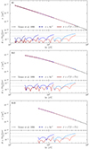 |
Fig. 1. Piece-wise power-law fits to the HI, HeI, and HeII photo-ionisation cross-section (top panels) and the associated relative error (lower panels). The black dotted line shows the cross-sections from Verner et al. (1996), the blue dashed lines a simple power-law fit, and the red solid lines a power-law series (Eq. 5). The horizontal dotted lines in the lower panels indicate relative errors of 1% and 10%. |
2.2. Discretising the source spectra
Observing typical source spectra such as the combined spectrum of multiple stars or the UVB, as shown in Fig. 2 for a simple stellar population (SSP) and Fig. 3 for the Haardt & Madau (2012) UVB, two main common features of their shapes becomes obvious. The first is the presence of jumps in intensity across the ionisation edges of H and He, and the second is the relatively constant slopes between these ionisation edges at a given time.
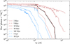 |
Fig. 2. Synthetic stellar population spectra between 1 and 200 eV for different population ages. The spectra are calculated with STARBURST99 (Leitherer et al. 2014) using the Padova AGB evolution tracks with solar metallicity and Kroupa (2001) IMF. The black line shows the PWPL reconstructed spectrum for a population age of 10 Myr. |
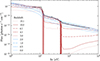 |
Fig. 3. Haardt & Madau (2012) UV background spectrum between 1 and 1000 eV for various redshifts ranging from z = 15.1 to 0.0. The black line shows the PWPL reconstructed spectrum at z = 3. |
In order to capture potential jumps across the ionisation edges we represent the spectrum at these energies with two distinct photon energies, one approaching the ionisation energy from the low-energy side and one from the high-energy side. For the HI ionisation energy of 13.6 eV these energies are denoted as 13.6− and 13.6+ eV, where the superscript + and − indicate the direction of approach. We further assume that the spectral shape within an ionising band can be described as power law. The slope of the individual power-law pieces is calculated on-the-fly for each receiving resolution element. In practise, we first add the attenuated photon fluxes at each considered photon energy, and calculate the spectral slope based on the combined intensities. This approach naturally follows spectral hardening within the typical ionisation bands, as the fluxes at every photon energy are attenuated according to their respective opacity. In contrast, in the PWC approximation the intensity within one ionising band is calculated based on a single effective opacity and thus is not able to capture any changes in the shape of the radiation filed due to frequency dependent absorption.
This representation of the spectrum leads to 6 considered photon energies in the range of 13.6 to 136 eV. We chose 136 eV as upper energy limit for the HeII ionising band (HeII-high), as this is the typical upper energy limit of popular stellar spectral synthesis codes, such as STARBURST99 (Leitherer et al. 2014) or SLUG (da Silva et al. 2012). An upper energy limit of 136 eV for the source spectra is insufficient to accurately capture the photo-ionisation and heating rates of helium, in particular HeII. This is especially true in cases were the high-energy spectral slope is positive, such as for the Haardt & Madau (2012) UVB at z ≳ 4, or in cases of strong spectral hardening. In order to improve the accuracy of the calculated HeII photo-ionisation rates, we additional consider high-energy photons at 500 eV (XUV). We additionally include one FUV band (5.6 − 11.2 eV) and two Lyman-Werner bands for photo-electric heating and for future inclusion of H2 chemistry, resulting in a total of ten photon energies. The black lines in Figs. 2 and 3 show the PWPL approximation of the spectrum of a SSP with a population age of 10 Myr and the UVB at z = 3, respectively. A comprehensive list of the considered photon energies is provided in Table 2.
Photon energies used in the PWPL approximation and their intended use cases.
2.3. Calculating photo-ionisation and heating rates
Combining our power-law approximations for the radiation field and ionisation cross-sections allows us to simplify Eqs. (1) and (2) into
 (6)
(6)
and
![Mathematical equation: $$ \begin{aligned} \mathcal{H} _{i} = \sum _j \int _{\nu _{\mathrm{min} ,j}}^{\nu _{\mathrm{max} ,j}}{F_j\, \nu ^{\alpha _j}\, {h}\left(\nu -\nu _{0,i}\right)\,\left[ {S\!}_{i,j}\,\nu ^{\beta _{i,j}} + T_{i,j}\,\nu ^{\beta _{i,j}+1}\right]\,\mathrm{d}\nu }, \end{aligned} $$](/articles/aa/full_html/2024/11/aa48164-23/aa48164-23-eq11.gif) (7)
(7)
where the integral is split into a sum over the broad ionising bands j, νmin, j and νmax, j are the lower and upper frequency bound of ionising band j as indicated in column one of Table 1, Fj is the photon flux in photons cm−2 s−1 Hz−1 and αj is the slope of the power-law spectrum within the broad band j, Si, j, Ti, j and βi, j are the fitting parameters of the power-law photo-ionisation cross-sections, given in Table 1, and ν0, i is the ionisation potential of species i. These expressions can be evaluated analytically for each broad band, leading to
![Mathematical equation: $$ \begin{aligned} \begin{aligned} \Gamma _{i} =&\sum _{j} F_j \\&\times \left\{ {S\!}_{i,j} \left[\frac{\nu _{\mathrm{max},j}^{\alpha _j+\beta _{i,j}+1} - \nu _{\mathrm{min},j}^{\alpha _j+\beta _{i,j}+1}}{\alpha _j+\beta _{i,j}+1}\right] + T_{i,j} \left[\frac{\nu _{\mathrm{max},j}^{\alpha _j+\beta _{i,j}+2} - \nu _{\mathrm{min},j}^{\alpha _j+\beta _{i,j}+2}}{\alpha _j+\beta _{i,j}+2}\right] \right\} \end{aligned} \end{aligned} $$](/articles/aa/full_html/2024/11/aa48164-23/aa48164-23-eq12.gif) (8)
(8)
and
![Mathematical equation: $$ \begin{aligned} \begin{aligned} \mathcal{H} _{i} =&\sum _{j}\, F_j\,{h} \times \left\{ T_{i,j}\left[ \frac{\nu _{\mathrm{max},j}^{\alpha _j+\beta _{i,j}+3}- \nu _{\mathrm{min},j}^{\alpha _j+\beta _{i,j}+3}}{\alpha _j+\beta _{i,j}+3} \right]\right. \\&+ \left({S\!}_{i,j} - T_{i,j}\nu _{0,i} \right) \left[\frac{\nu _{\mathrm{max},j}^{\alpha _j+\beta _{i,j}+2}- \nu _{\mathrm{min},j}^{\alpha _j+\beta _{i,j}+2}}{\alpha _j+\beta _{i,j}+2} \right] \\&\left.- {S\!}_{i,j}\,\nu _{0,i}\, \left[ \frac{\nu _{\mathrm{max},j}^{\alpha _j+\beta _{i,j}+1} - \nu _{\mathrm{min},j}^{\alpha _j+\beta _{i,j}+1}}{\alpha _j+\beta _{i,j}+1} \right] \right\} . \end{aligned} \end{aligned} $$](/articles/aa/full_html/2024/11/aa48164-23/aa48164-23-eq13.gif) (9)
(9)
The approximations Eqs. (8) and (9) are considerably faster to evaluate than Eqs. (1) and (2) as the integral does not need to be numerically evaluated on a high-frequency resolution grid.
Unlike to the PWC approximation, with the PWPL spectral reconstruction it is possible to calculate the intensity of the radiation field at any frequency between the band edges. This enables us to calculate precise ionisation rates of for metal lines.
3. Model validation
3.1. Instantaneous ionisation and heating rates
In order to validate the PWPL approximation we computed the instantaneous photo-ionisation and heating rates for HI, HeI, and HeII according to Eqs. (8) and (9) and compared the results to the numerical integral of Eqs. (1) and (2) in the energy range 13.6 ≤ hν/eV ≤ 500 and to the PWC approximation. We performed this test for two typical source types with time depended spectra, namely the UVB and a 106 M⊙ star cluster at a distance of 100 pc. For the first case we used the Haardt & Madau (2012) UVB spectrum over the full published redshift range from z = 15 to 0. For the second case we calculated the intensities of the stellar sources in each bin based on synthetic spectra of a SSP derived with STARBURST99 (Leitherer et al. 2014) using the Padova AGB stellar evolution tracks for solar metallicity. We assumed the population follows the Kroupa (2001) IMF with a lower and upper mass limit of 0.1 and 100 M⊙, respectively, and ages between 1 Myr and 13 Gyr.
Due to absorption and emission features in the source spectra, as well as the fact that the source spectra do not actually follow piece-wise power laws, the integrated intensity within one ionising band based on a power law between the edges of the ionising band is not equal to the intensity of the source spectrum over the same energy interval. Typically, this leads to an underestimation of the intensity within the PWPL approximation. To correct for the mismatch in photon number, we scaled the number of photons in the PWPL input spectrum, so that the actual number of photons in an ionising band of the source spectrum is equal to the number of photons in the power-law reconstruction while keeping the power-law slope constant. This also ensures that the integrated number of photons in each ionising band emitted from the source are identical in the PWPL and PWC calculations. For the PWC calculations, we used 3 ionising bands with their boundaries at 13.6, 24.6, 54.4 and 500 eV and the same effective photo-ionisation cross-sections weighted by photon number as used in Kannan et al. (2022).
We compared the photo-ionisation (top panels) and heating (bottom panel) rates for the Haardt & Madau (2012) UVB (left) and the SSP (right) calculated with the PWPL (red lines), PWC (blue lines) to the numerical integral of Eqs. (1) and (2) (black lines) in Fig. 4. For both test cases the PWPL follows the shape of the numerical integral closely, while the PWC approximation has the tendency to produce higher ionisation and heating rates.
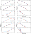 |
Fig. 4. Photo-ionisation rate (top) and photo-heating rate (bottom), for a redshift dependent uniform Haardt & Madau (2012) UVB spectrum (left) and an aging SSP with Mcl = 106 M⊙ at a distance of 100 pc (right). The blue line shows the ionisation and heating rate for the common PWC approximation of the radiation field in combination with a constant σeff. The red line corresponds to our new PWPL approximation for the radiation field in combination with the power-law photo-ionisation cross-section (Eq. 6). |
The PWPL approximation simultaneously predicts the photo-ionisation and heating rates accurately in the UVB case, with mean errors of 0.005, 0.11 and 0.04 dex for HI, HeI and HeII ionisation rates, respectively, and 0.004, 0.03 and 0.08 dex for the heating rates. As apparent from the left panels of Fig. 4, the PWC approximation fails to predict photo heating rates in this test, with mean errors of 0.44, 0.66 and 2.32 dex for HI, HeI and HeII photo heating rates, respectively. The mean errors for the photo-ionisation rates of the three species are 0.08, 0.02 and 1.15 dex. We show the distribution of relative errors for the PWC (blue lines) and PWPL (red lines) approximations relative to the numerical integral of Eqs. (1) and (2), for the ionisation (top panel) and heating (bottom panel) rates of HI (solid), HeI (dashed) and HeII (dot-dashed) for the redshift dependent UVB case in the left panel of Fig. 5. We define the relative error as
 (10)
(10)
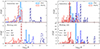 |
Fig. 5. Relative error distribution for the ionisation (top) and heating (bottom) rates, for the PWPL (reds) and PWC (blues) approximation. The left panel corresponds to the redshift dependent UVB spectrum and the right panel to the age dependent SSP spectrum for population ages below 8 Myr. Different line styles show the error distribution for HI (solid), HeI (dashed), and HeII (dot-dashed). The errors are calculated relative to the numerical integration of Eqs. (1) and (2). |
where X is either the photo-ionisation or heating rate, we assume the numerically integrated values represent the true rates.
As the SSP ages, its spectral shape changes, which cannot be captured by the pre-calculated cross-section in the PWC case. This results in a varying accuracy, where the deviation from the expected rates increases with population age, for the chosen pre-calculated cross-sections. The calculated photo-ionisation and heating rates of the PWPL approximation closely follow the expected values (Fig. 4 right). Whereas the PWC approximation overestimates both by several orders of magnitude. The spectral shape changes during the evolution of the SSP cannot be captured by the pre-calculated cross-sections in the PWC case. This results in a population age dependent accuracy, where the deviation from the expected rates increases with population age, for the chosen pre-calculated cross-sections. As the population ages, the number of emitted high-energy photon decreases, starting at the highest energies and successively progressing to lower energies (see Fig. 2). Due to the discretisation of the source spectrum, for both the PWC and PWPL methods, the highest energy bands still hold photons, including at energies where the original sources emit little to no photons. As the heating rate is governed by the excess energy per ionisation, the term h(ν − ν0, i) in Eq. (2), even a small number of high-energy photons can significantly increase the photo-heating rate. Similar behaviour is to be expected for any approximation of the radiation field, which relies on a limited number of radiation bands. This causes huge nominal errors, but the effect is negligible as at this point the heating rates are already ∼10 orders of magnitude lower compared to a young stellar population. This effect is particularly apparent in the HeII ionisation rates for population ages ≳8 Myr (bottom right panel of Fig. 4). For this reason we only show the error distribution of SSP ages below 8 Myr in the right panel of Fig. 5.
We note that the behaviour of the PWC approximation could be improved by carefully evaluating  for each of the different spectral shapes in the test. This approach is not practical in full-scale RT simulations, even in this limited test with combined 160 different spectra the time needed to calculate all 960 cross-sections by far exceeds the time needed to calculate the ionisation and heating rates.
3.2. Expanding HII-region
The expansion of an HII-region in pure hydrogen is a typical test case used to assess the performance of radiative transfer codes (e.g. Gnedin & Abel 2001; Iliev et al. 2006, 2009; Rosdahl et al. 2013; Grond et al. 2019; Kannan et al. 2019). Thereby, the density is assumed to be constant, the radiation field is represented by a single ionising band and recombination is limited to case B. In the classic Strömgren sphere test the temperature is kept constant, although usually a second test with varying temperature is performed as well.
We implemented our new PWPL spectral reconstruction method for the radiation field into an early test version of TREVR2 (Wadsley et al. 2024), the new radiative transfer method of the Tree-SPH code GASOLINE2 (Wadsley et al. 2017). TREVR2 is a fast reverse ray tracing algorithm with 𝒪(Nactive log2 N) computational cost, here Nactive is the number of currently active receiving particles and N = Nstar + Ngas is the total number of star and gas particles. It performs the ray tracing from the receiver to the sources along HEALPix (Górski et al. 2005) cones.
We performed a multi-band version of the expanding HII-region test with variable temperature, dropping the restriction of only having one radiation band and did not restrict recombination to case B. Additional to the pure hydrogen case, we also present results for a primordial gas mixture of hydrogen and helium, with a helium mass fraction of 23.6%. A single source of photons was placed in the centre of the simulation box with a side length of 16 kpc. We used 643 gas particles to model the constant density medium with nH = 10−3 cm−3 and an initial gas temperature of T = 100 K. For the primordial mixture case we kept nH = 10−3 cm−3 and added mass to the particles so that the helium mass fractions reached the aforementioned 23.6%, resulting in nH + He ≈ 1.07 × 10⁻³ cm−3. Following Katz (2022), we used a black body with TBB = 104.759 K and a luminosity of LBB = 104.324 L⊙ as source, which resembles a 15 M⊙ main-sequence star (Schaerer 2002). As for the previous tests, we scaled the number of photons at the PWPL energies so that the total number of photons in the ionising bands equals the integrated number of photons in the same energy interval within the PWPL approximation, while keeping the power-law slope constant.
We compared our PWPL results to the PWC approximation and comparison runs from CLOUDY (version 17.02, Ferland et al. 2017). For the PWC runs we calculated  according to Eq. (3) for the considered black-body spectrum. For the CLOUDY calculations we deactivated molecular chemistry and dust physics as both are not considered with in the chemical network of GASOLINE2.
We illustrate how the PWPL spectral reconstruction method follows the change in spectral shape of the initial black-body source as it is absorbed by the surrounding medium in Fig. 6. We compare the reconstructed spectrum of the PWPL approximation with the expected spectrum according to CLOUDY and the three-band PWC approximation at column densities NHI = 1017, 1018, and 5 × 1018 cm−2 corresponding to an optical depth at 13.6 eV of τ13.6 ≈ 0.64, 6.4 and 31.8, from the source, for the pure H (top) and primoridal H and He mixture (bottom) case. At low column density the medium is fully ionised resulting in an optically thin medium and the reconstructed spectrum agrees well with the expected spectrum. As radiation propagates further from the source it is absorbed more at the low-energy end of an ionising band and the flux maximum within one broad band shifts from the low-energy side towards the high-energy end. In the PWPL approximation the fluxes are calculated at the ends of the ionising bands, this allows the PWPL spectral reconstruction to follow the changing slope of the spectrum within the classical ionising bands. In case the maximum of the radiation field lies between the bounding energies of an ionising band the number of photons in the reconstructed spectrum will be lower compared to the expected number in the band, this leads to an underestimation of the ionisation rate and thus a higher neutral fraction. This process accumulates with distance from the source and is particularly visible between 24.6 and 54.4 eV (HeI ionising band) in the right panels of Fig. 6.
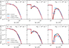 |
Fig. 6. Reconstructed radiation field after t = 1500 Myr, at column densities of NHI = 1017, 1018, and 5 × 1018 cm−2 (from left to right) from the source, for the pure hydrogen (top) and primordial hydrogen and helium mixture (bottom) case. The black line denotes the CLOUDY reference runs, the red lines show the reconstructed spectrum using the PWPL approximation and the blue line represents the classic three-band PWC approach. For illustrative purposes, we represent the spectral shape of the three-band PWC case as scaled intervals of the initial black-body spectrum, while in practice it is treated as a delta function at the effective frequency of each band. |
In the PWC approximation the spectral shape is encoded in the effective photo-ionisation cross-section, which is representative for an effective photon energy in a given ionisation band. We illustrate this by representing the PWC spectrum (blue lines) in Fig. 6 as scaled down intervals of the original black-body spectrum for which  was calculated. In practice, the PWC approximation uses a single intensity value at the effective photon energy. The black-body pieces in Fig. 6 are scaled such that the integrated flux within one ionising band is conserved. It becomes obvious that the PWC effective spectral shape does not agree with the expected spectrum once absorption becomes important in shaping the spectrum of the incident radiation field. The effective PWC spectrum in this test favours photons at the low-energy edge of one band, these photons are more likely to ionise the gas as the cross-sections at lower energies are larger. This leads to a greater spatial extend of the ionised bubble compared to the PWPL case, as can be seen in Figs. 7 and 8.
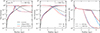 |
Fig. 7. Expanding HII region in a pure hydrogen environment with nH = 10−3 cm−3 and an initial temperature of 100 K. The hydrogen ion fractions (HI solid and HII dashed lines) after t = 100 (1500) Myr is shown in the left (middle) panel. Red lines show the results using the ten-band PWPL, blue lines using the three-band PWC approximation, and the black lines represent the CLOUDY equilibrium solution. The thin dashed line represents an ion fraction of 50%. The right panel shows the temperature profile of the HII region after t = 100 and 1500 Myr as dashed and solid lines, respectively. |
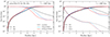 |
Fig. 8. Expanding HII region in a primodial mixture of hydrogen and helium environment with nH = 10−3 cm−3 and an initial temperature of 100 K. The hydrogen ion fractions (HI solid and HII dashed lines) after t = 1500 Myr is shown in the left panel. The right panel shows the helium ion fractions (HeI solid, HeII dashed, and HeIII dotted lines) after t = 1500 Myr. The thin dashed line represents an ion fraction of 50%. |
In Fig. 7 we show the resulting hydrogen ion fractions for the pure H case during the rapid expansion phase of the HII region, after t = 100 Myr (left) and after t = 1500 Myr when the final equilibrium has been reached. The right panel shows the temperature profile of the HII region at the same times. It closely follows the CLOUDY comparison run until the knee of the temperature profile, where the photo-heated region transitions to the initially cold surrounding medium. This difference in the temperature profile at large distances beyond approximately 5 kpc from the central source is a result of inherently different approaches to the chemistry solver. GASOLINE2 uses a non-equilibrium chemical network to heat the initially cold (100 K) gas, while CLOUDY directly calculates the equilibrium state. In Fig. 8 we show equilibrium hydrogen (left) and helium (right) ion fraction, of the primordial H and He case.
We note that we did not attempt to fully reproduce CLOUDY results. This would require to adjust the cross-sections and reaction rates to those used in CLOUDY, as attempted in Katz (2022). Even then we would potentially be limited by the different approaches of the chemical network, the geometry of the problem (1D in CLOUDY versus 3D in GASOLINE2), the spatial resolution or the spectral range and resolution. Therefore, we merely use the CLOUDY calculations as qualitative guide to interpret our test results. It is further worth pointing out that there even exist quantitative differences between various PDR codes (e.g. Röllig et al. 2007). We investigated the impact of resolution in Appendix A, and show that our results are well converged.
3.3. Uniform background in an homogeneous box
This test is designed to show case how we treat background radiation for cosmological zoom-in simulations and the implications for the simulation box size. As in the original version of TREVR (Grond et al. 2019), we use virtual background sources distributed along a spiral on a sphere centred on the centre of the simulation box with its radius equal to the half of the box width as sources of the UVB. This distribution of background sources is intended to mimic a spherical shell emitting light towards its centre. The flux received from the shell at any position within this shell can be calculated by
 (11)
(11)
where L is the luminosity of the emitting shell, R is the shell radius and r the distance from the shell’s centre. Although the background sources are treated identical to Grond et al. (2019) it is worth illustrating how the background radiation field is modelled, as a realistic treatment of the UVB has a severe impact on cosmological zoom-in simulations as discussed in Sect. 4.
We used a low-resolution (323 dark matter and gas particles) cosmological volume of 100 comoving Mpc per side, with H0 = 67.8 km s−1 Mpc−1, Ωm = 0.3086, ΩΛ = 0.6814 and Ωb = 0.048 cosmology. As this test only considers optically thin radiative transfer and no force calculations, the number of particles, their mass and actual position are not relevant, the gas particles merely serve as tracers of the radiation field at their respective location. In the optically thin case the behaviour is independent of photon energy, therefore we choose to only show the results at 13.6+ eV (HI-low). For this test we used 128 background sources, which emit light according to the UVB spectrum of Haardt & Madau (2012).
In the left panel of Fig. 9 the distribution of background sources within the simulation volume is illustrated for 128 emitters, with the point size corresponding to the distance from the viewer. The right panel of Fig. 9 shows the resulting radiation field at 13.6+ eV (HI-low) in a thin slice through the centre of the simulation volume. The brighter areas indicate the positions of the background sources. The red circles indicate the regions within which the flux is below 1.5 (dotted), 1.25 (dot-dashed) and 1.1 (dashed) times the central flux, corresponding to r = [0.43, 0.36, 0.26]×Lbox, respectively. In cosmological zoom-in simulations, the relatively small high-resolution region of interest is typically located at the centre of the simulation volume, where the radiation field is only marginally deviating from the expected background intensity and exhibits little scatter.
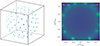 |
Fig. 9. Uniform background test. Left: Illustration of the distribution of background sources within the simulation box for 128 background emitters. The virtual background emitters are distributed along a spiral on a sphere centred on the centre of the simulation box; the point size corresponds to the distance from the viewer. Right: Incident radiation field at 13.6+ eV (HI-low) as experienced by gas particles in the uniform background test in a thin slice through the centre of the simulation box for the Haardt & Madau (2012) UVB at redshift 0 and 128 background sources. The dashed, dot-dashed, and dotted circles indicate where the radiation field is within 10%, 25%, and 50% of the expected central flux, respectively. The corresponding radii are, from the centre out, [0.26, 0.36, 0.43]×Lbox. |
4. Post-processing MUGS2 g1536
Here we present the results of post-processing seven snapshots of the zoom-in galaxy g1536 form the McMaster Unbiased Galaxy Simulations 2 (MUGS2, Keller et al. 2016). The simulation was originally run with the tree-SPH code GASOLINE2 (Wadsley et al. 2017) using a WMAP3 ΛCDM cosmology with H0 = 73 km s−1 Mpc−1, Ωm = 0.24, ΩΛ = 0.76, Ωb = 0.04 and σ8 = 0.76 (Spergel et al. 2007). In the high-resolution zoom region the particle masses are 1.1 × 10⁶ M⊙ and 2.2 × 10⁵ M⊙ for dark matter and gas, respectively, and the gravitational softening length was set to 312.5 pc. These simulations include a non-equilibrium chemical network for H and He, and equilibrium metal line cooling under the influence of a uniform and redshift dependent UVB as described in Shen et al. (2010). Stars are formed stochastically once a gas particles has become sufficiently cold (T < 1.5 × 10⁴ K) and dense (n > 9.3 cm−3) at a rate proportional to the local free-fall time
 (12)
(12)
where an efficiency parameter c⋆ = 0.1 is used. Supernova (SN) feedback is treated according to the superbubble model (Keller et al. 2014). In this scheme, gas particles affected by SN feedback temporarily become two phase particles, where one phase represents the SN heated portion of the particle while the other phase is the cold ISM. The transition between the hot and cold phase is governed by thermal conduction. Both phases have their individual mass, density and specific energy. This allows separate cooling in each phase, eliminating the need for a cooling shut-off as is often used in single phase feedback models to prevent over-cooling.
At z = 0 MUGS2 g1536 resembles an almost bulgeless disk galaxy with a total mass of 7 × 10¹¹ M⊙ of which 5.1 × 10¹⁰ M⊙ are attributed to gas and 6.0 × 10¹⁰ M⊙ to stars, resulting in a baryon fraction fb = 15.9%. This galaxy was used in Keller et al. (2015) to demonstrate the differences and impact of the superbubble feedback description compared to the blastwave model from Stinson et al. (2006), which was used in the original MUGS simulations (Stinson et al. 2010).
We post-processed seven snapshots between z = 6.0 and 0.0, with their basic properties listed in Table 3, using GASOLINE2 and the new ray tracing module TREVR2 with our PWPL approximation for the radiation field. In order to study the impact of radiation on the gas phase of g1536 we deactivated gravity, hydrodynamics, star formation and stellar feedback in the post-processing runs. Excluding these physical processes disables significant heating processes, such as shock heating and the energy deposition by SN into the ISM. To counteract the potentially fast cooling of feedback and shock heated gas, we kept the temperature for particles with T ≥ 2 × 10⁴ K constant but evaluated their ionisation states under the influence of the radiation field. We evolved the simulation for 1000 steps, equivalent to ∼13 Myr, in order to reach a steady ionisation state. We considered stars and a homogeneous UVB as sources of radiation, with their spectra as described in Sect. 3.1. The UVB was represented with 128 virtual sources for which we kept the redshift constant at the value of the respective snapshot. The luminosity of each star particle was calculated individually based on the age of stellar population, which we kept fixed throughout the post-processing runs.
Properties of the most massive progenitor of MUGS2 g1536 at various redshifts.
In Fig. 10 we compare the phase-space distribution of gas particles of the most massive progenitor of g1536 before (left) and after post-processing (right) at redshift 6, 2 and 0.1 (from top to bottom). At early times (z = 6) the UVB ionises and heats all of the gas to T ≈ 104 K in the initial run, due to its uniform treatment. Simultaneously small burst of star formation create a small amount of SN heated gas with T > 104 K. During post-processing the radiation emitted by the UVB has to propagate through the IGM and CGM, where large portion of the UVB photons get absorbed before reaching the inner CGM or the ISM. This results in a large portion of the ISM remaining cold (T < 100 K) and neutral, as it is shielded against the UVB. After post-processing the total neutral mass fraction (MHI + MHeI)/Mgas within the halo of g1536 is 56% whereas initially it was only 8%.
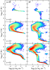 |
Fig. 10. Density-temperature phase-space of the most massive progenitor of g1536 at redshift 6, 2, and 0.1 (from top to bottom). The left panels show the original distribution (i.e. the initial condition for the post-processing run and the right panels show the distribution after the post-processing). The horizontal segregation at T = 2 × 10⁴ K, is artificial due to disabling of cooling for high temperature gas (see text for details). |
At z = 2, the UVB reaches its maximum strength, keeping the majority of gas ionised in the initial run, while simultaneously the amount of SN heated gas increased. Shortly after this snapshot, g1536 experiences a star burst. First indications of this event can be seen in the formation of a thin extension of the distribution towards high gas densities. Although the UVB is at its strongest, the ISM remains well shielded after post-processing. At temperatures between 7 × 10³ and 3 × 10⁴ K and densities above 1 cm−3 a population of locally ionised HII regions, with fHII > 80%, is established around young star clusters. At z = 0.1 g1536 is in a phase of ongoing star formation, reflected in the cool (T < 104 K) and dense (n > 10 cm−3) gas, which will be converted into stars during the following time steps. In the RT run recent and ongoing star formation is further reflected in the increased amount of particles in the HII region phase. In Fig. 11 we illustrate the spatial alignment of locally ionised gas with fHI > 80%, populating this distinct region in the phase-space (ρ ≥ 1 cm−3 and 7 × 10³ ≤ T/K ≤ 3 × 10⁴), with the location of young stars. The red contours show the locations of highly ionised gas particles at z = 0.1, overlain onto a mock composite image of stars, where brighter blue regions are indicative of young stellar populations. The horizontal segregation at T = 2 × 10⁴ K in the right panels of Fig. 10 is an artefact caused by disabling cooling of high temperature gas.
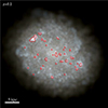 |
Fig. 11. Location of photo-ionised gas in g1536 at z = 0.1 overlaid onto a mock i-, v-, and b-band composite image of the stellar component, viewed face on. The luminosity of the stars are calculated using Marigo et al. (2008) stellar populations, the effect of dust extinction is not included. Particles constituting the illustrated HII regions have fHII > 80%, ρ ≥ 1 cm−3 and 7 × 10³ ≤ T/K ≤ 3 × 10⁴. |
The persistent existence of cold gas (T ≲ 100 K) points to a possibly significantly altered star formation history of g1536 in a fully self-consistent cosmological RT simulation. In the original run from Keller et al. (2015) star formation happens in short (< 7 Myr) bursts with rates up 10 M⊙ yr−1 and typically below 5 M⊙ yr−1. The phase diagram after post-processing gives rise to the possibility of more continuous SF at higher rates, due to the available amount of cold and dense gas. However, it is difficult to predict how the increased amount of cold gas impact the SFH without self-consistent RT simulations. More cold gas can lead to stronger bursts of star formation, but in turn stellar feedback is also stronger, which could ultimately be more destructive.
As already seen in the phase-space diagrams, the amount of cold, and neutral gas, increases significantly after RT post-processing. We investigated the change in ion mass for hydrogen and helium relative to the initial ion mass before post-processing in Fig. 12. At z = 2, the increase of neutral hydrogen mass is at its maximum with seven times more neutral hydrogen after post-processing. In contrast to the strong change in the mass of neutral ions, the mass of HeIII remains almost unchanged, as the high-energy photons required to fully ionise helium have a long mean free path, and are able to penetrate deep into the ISM of g1536. The ion masses of hydrogen and helium before and after post-processing are provided in Table 4. The redshift evolution of the increase of neutral and decrease of ionised mass follows the intensity of the UVB, indicating that most of the change is related to the treatment of the UVB. In the original MUGS2 run all but the densest and coldest gas in the ISM is ionised by the uniform UVB, whereas in the RT post-processing run gas with n ≳ 10−2 cm−3 is shielded against the UVB, as can be seen in Fig. 10 and was found in previous studies (e.g. Gnedin 2010; Rahmati et al. 2013). Stars in the post-processing run ionise parts of the ISM, which have previously been ionised by the uniform UVB, but are not able to entirely compensate for the reduced intensity of the UVB. The assumption of a spatial uniform and instantaneous UVB without a correction for self-shielding, as used in the original MUGS2 run, underestimates the amount of neutral gas in and around a galaxy.
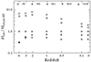 |
Fig. 12. Ion mass relative to the initial ion mass before RT post-processing, for the considered species of the chemical network, of the most massive progenitor of g1536 at various redshifts. |
Neutral and ionised H and He mass of the most massive progenitor of MUGS2 g1536 at various redshifts before and after RT post-processing.
Figure 13 shows that most of the additionally formed HI gas is located in the CGM of g1536 at z = 2. This holds true at all examined redshifts. In the RT post-processing run the UVB light has to propagate inwards from the edge of the simulation box, thereby it is partially absorbed, reducing its ability to penetrate deep into the halo of g1536. Further, RT post-processing revealed a large reservoir of neutral gas in a small companion and its associated long (up to ∼40 kpc) ram pressure stripped tail with NHI > 1020 cm−2. Although visible in total gas surface density (see Fig. 14), with Σgas ≈ 10 M⊙ pc−2, this feature remains hidden in the original MUGS2 run, as the instantaneous and uniform treatment of the UVB ionises and heats all but the densest gas.
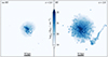 |
Fig. 13. Face-on projection of the neutral hydrogen density (NHI) in a region with 100 kpc per side centred on the most massive progenitor of g1536 at z = 2 before (left) and after (right) RT post-processing. |
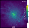 |
Fig. 14. Face-on projected total gas density (Σgas) in a region with 100 kpc per side centred on the most massive progenitor of g1536 at z = 2. |
We investigate the impact of tree-based RT with cell averaged quantities on the amount of neutral and ionised gas in Appendix B.
5. Discussion
In this work we presented a new method to reconstruct the spectral shape of the incident radiation field in RT simulations to accurately calculate photo-ionisation and heating rates. Thereby, we represent the intensity of the source spectrum at the ionisation energies of H and He with two distinct energies, one approaching the ionisation energy from the low and one from the high-energy side and assume that the spectra follow a power law between these characteristic energies. Using two frequencies at each ionisation edge allows to track jumps in intensity across these edges as illustrated in Fig. 6. We represent the photo-ionisation cross-sections as piece-wise power laws, instead of using a single value at an effective frequency. These two assumptions enable us to analytically evaluate photo-ionisation and heating rates for any combination of source spectra, and is therefore well suited for hydrodynamic simulations with on-the-fly radiative transfer. It does not only allow to self-consistently combine radiation from different sources, each with its individual spectrum, but also follows spectral hardening within the typical ionising bands naturally. Furthermore, it is possible to calculate the intensity of the radiation field at any frequency, which is crucial for accurate predictions of the ionisation state of metals. We explore the impact of the radiation field approximation on the abundance of various metal ions in the CGM in an upcoming work.
The PWPL spectral reconstruction method is applicable in any RT code. We choose to use TREVR2 for our tests due to its Nactive log2(N) scaling and the low additional cost of performing multi-band RT. Using ten bands only increased the time required for RT by a factor of ∼1.3 compared to a single band.
We validate the PWPL spectral reconstruction method by calculating instantaneous photo-ionisation and heating rates for the Haardt & Madau (2012) UVB and an aging SSP. Thereby, we find excellent agreement between the PWPL method and the full frequency dependent integral over the entire redshift range of the UVB spectrum and considered species, with typical errors bellow 10%. For the aging SSP we find typical deviations from the frequency dependent integral of the photo-ionisation rate below 0.1 dex, within the first 8 Myr of stellar evolution. As the population ages, the error increases to 0.5 dex over a range of ∼20 dex in photo-ionisation rates, at this point the ionisation rates have already decreased by more than 5 dex from their initial values. Qualitatively the results are similar for the heating rates, where strong deviations arise after about 8, 15, 100 Myr for the HeII, HeI and H heating rates, respectively. This is attributed to the discretisation of the stellar spectra into a finite number of bins, regardless of the number of considered bands. As the population ages the intensity of high-energy photons gradually decreases starting at the highest energies (see Fig. 2). If the source spectrum only partially reaches into an ionising band, for example if the HeII band (54.4 − 136 eV) is truncated at 100 eV, the photons get artificially distributed throughout the whole band. In the PWC approximation the photons would be smeared out over the full energy range of the HeII band, while in the PWPL reconstruction the spectral slope would be calculated between the HeII-low energy (54.4+ eV) and the zero-intensity in the HeII-high energy (136 eV). Therefore, both approximations consider more higher energy photons than are actually present in the input spectrum, resulting in an overestimation of the photo-heating rates. We have chosen to conserve the number of photons per broad band of the input spectrum, amplifying this effect. If we would have chosen to conserve the total energy per band the errors in the photo-heating rates would be smaller, but at the cost of increasing the errors in the photo-ionisation rates. However, in applications we do not expect these larger errors in the heating rates to have a significant impact, as the errors are nominally large but at heating rates which are orders of magnitude below the zero-age rates.
We illustrate how the spectrum changes its shape as light travels through the medium of an HII-region, illuminated by a single source (see Fig. 6). For optical depths τ ≲ 10 the spectral shape can be recovered well. As the optical depth rises further the PWPL reconstruction underestimates the number of ionising photons, as the transmitted spectrum is no longer well represented by simple piece-wise power laws. Adding additional energies between the ionisation edges and/or using a higher order reconstruction are possible ways to minimise this effect, we leave such improvements for future exploration. We expect this effect to be less prominent in situations with multiple source with different spectral shapes.
By post-processing MUGS2 g1536, an almost bulgeless, star forming galaxy with Mvir = 7.5 × 10¹¹ M⊙ at z = 0, we show the importance of radiative transfer for future (zoom-in) simulations of galaxy evolution. The inclusion of radiation leads to a realistic multi-phase structure of the ISM, consisting of a cold (T < 100 K), a hot (T > 104 K) and a warm (T ≈ 104 K) phase. The warm phase is co-spatial with recently formed stars which heat and ionise their surrounding gas with their intense UV radiation. Further, we find large differences in the distribution of neutral gas in the CGM of g1536. In the comparison run from Keller et al. (2016), which utilises spatially uniform photo-ionisation and heating rates for the UVB, only the densest and coldest gas, with recombination rates exceeding the photo-ionisation rates of the UVB, are able to remain neutral. This leads to an almost completely ionised CGM, with only a small amount of neutral gas extending beyond the ISM. As the radiation emitted by the UVB sources has to propagate through the halo of the galaxy, whereby it is partly absorbed by the intervening matter, a much larger circumgalactic reservoir of neutral gas is present. This neutral gas reservoir extends far beyond the stellar disk, as commonly observed in galaxies (e.g. Tumlinson et al. 2013; Wang et al. 2016) or around z = 2 quasars (e.g. Prochaska et al. 2013). Additionally, we find large neutral fractions in a ram pressure stripped tail of an in-falling dwarf galaxies at z = 2. The tail is visible in the total gas surface density in the original run (see Fig. 14), but is completely ionised by the UVB. Furthermore, we find that a series of small satellite halos can retain neutral gas until redshifts below 2. These changes in the structure and distribution of neutral gas in the CGM show the importance of radiation and a proper treatment of the UVB for studies of galaxy evolution in general, and in particular for studies of the CGM.
We note that the highlighted differences before and after RT post-processing are only to be considered illustrative for the potential changes in galaxy simulations if RT is included and the UVB is treated appropriately. All the presented changes in the structure of the galaxy and its CGM indicate a significantly altered star formation history. In preliminary tests we saw star formation rates increased by a factor of 5 to 10 compared to the original run without RT. This in turn effects the stellar feedback and radiation field, and thus the dynamics of the whole system.
These changes and their impact on the gas properties of MUGS2 g1536 show the need for fully self-consistent cosmological (zoom-in) RT simulations in order to further develop our understanding of galaxy evolution. Thereby the RT code and the used approximations made for the radiation field and related quantities must allow for the combination of sources with different spectra and include a realistic treatment of UVB – as it is possible with our new PWPL spectral reconstruction method. In upcoming works, we will present such cosmological zoom-in simulations of galaxy evolution with on-the-fly RT, including a realistic treatment of the UVB, employing our PWPL spectral reconstruction method.
An upper limit of ∞ eV for the HeII band is often used to indicate that this band includes all radiation until the highest considered photon energies, while in reality the upper limit is usually around 136 eV, which is the maximum photon energy considered by stellar population synthesis codes.
Acknowledgments
We thank the referee Nick Gnedin for valuable comments which helped us to improve the presentation of the paper. BB and SS acknowledge support from the Research Council of Norway through NFR Young Research Talents Grant 276043. SS also acknowledge support from the European High Performance Computing Joint Undertaking (EuroHPC JU) and the Research Council of Norway through the funding of the SPACE Centre of Excellence (grant agreement N0 101093441). JW is supported by a Discovery Grant from NSERC of Canada. Parts of the computations were performed on resources provided by Sigma2 – the National Infrastructure for High Performance Computing and Data Storage in Norway and on the Niagara supercomputer at the SciNet HPC Consortium. SciNet is funded by: the Canada Foundation for Innovation; the Government of Ontario; Ontario Research Fund – Research Excellence; and the University of Toronto.
References
- Agertz, O., Pontzen, A., Read, J. I., et al. 2020, MNRAS, 491, 1656 [Google Scholar]
- Aubert, D., & Teyssier, R. 2010, ApJ, 724, 244 [NASA ADS] [CrossRef] [Google Scholar]
- Blaizot, J., Garel, T., Verhamme, A., et al. 2023, MNRAS, 523, 3749 [NASA ADS] [CrossRef] [Google Scholar]
- da Silva, R. L., Fumagalli, M., & Krumholz, M. 2012, ApJ, 745, 145 [CrossRef] [Google Scholar]
- Decataldo, D., Shen, S., Mayer, L., Baumschlager, B., & Madau, P. 2024, A&A, 685, A8 [NASA ADS] [CrossRef] [EDP Sciences] [Google Scholar]
- Ferland, G. J., Chatzikos, M., Guzmán, F., et al. 2017, Rev. Mex. Astron. Astrofis., 53, 385 [NASA ADS] [Google Scholar]
- Fielding, D. B., Tonnesen, S., DeFelippis, D., et al. 2020, ApJ, 903, 32 [NASA ADS] [CrossRef] [Google Scholar]
- Garcia, F. A. B., Ricotti, M., Sugimura, K., & Park, J. 2023, MNRAS, 522, 2495 [NASA ADS] [CrossRef] [Google Scholar]
- Gnedin, N. Y. 2010, ApJ, 721, L79 [NASA ADS] [CrossRef] [Google Scholar]
- Gnedin, N. Y. 2014, ApJ, 793, 29 [CrossRef] [Google Scholar]
- Gnedin, N. Y., & Abel, T. 2001, New Astron., 6, 437 [NASA ADS] [CrossRef] [Google Scholar]
- González, M., Audit, E., & Huynh, P. 2007, A&A, 464, 429 [Google Scholar]
- Górski, K. M., Hivon, E., Banday, A. J., et al. 2005, ApJ, 622, 759 [Google Scholar]
- Grond, J. J., Woods, R. M., Wadsley, J. W., & Couchman, H. M. P. 2019, MNRAS, 485, 3681 [NASA ADS] [CrossRef] [Google Scholar]
- Haardt, F., & Madau, P. 2012, ApJ, 746, 125 [Google Scholar]
- Iliev, I. T., Ciardi, B., Alvarez, M. A., et al. 2006, MNRAS, 371, 1057 [NASA ADS] [CrossRef] [Google Scholar]
- Iliev, I. T., Whalen, D., Mellema, G., et al. 2009, MNRAS, 400, 1283 [NASA ADS] [CrossRef] [Google Scholar]
- Jeon, M., Pawlik, A. H., Bromm, V., & Milosavljević, M. 2014, MNRAS, 440, 3778 [NASA ADS] [CrossRef] [Google Scholar]
- Kannan, R., Vogelsberger, M., Marinacci, F., et al. 2019, MNRAS, 485, 117 [CrossRef] [Google Scholar]
- Kannan, R., Garaldi, E., Smith, A., et al. 2022, MNRAS, 511, 4005 [NASA ADS] [CrossRef] [Google Scholar]
- Katz, H. 2022, MNRAS, 512, 348 [NASA ADS] [CrossRef] [Google Scholar]
- Keller, B. W., Wadsley, J., Benincasa, S. M., & Couchman, H. M. P. 2014, MNRAS, 442, 3013 [NASA ADS] [CrossRef] [Google Scholar]
- Keller, B. W., Wadsley, J., & Couchman, H. M. P. 2015, MNRAS, 453, 3499 [Google Scholar]
- Keller, B. W., Wadsley, J., & Couchman, H. M. P. 2016, MNRAS, 463, 1431 [Google Scholar]
- Kimm, T., Katz, H., Haehnelt, M., et al. 2017, MNRAS, 466, 4826 [NASA ADS] [Google Scholar]
- Kroupa, P. 2001, MNRAS, 322, 231 [NASA ADS] [CrossRef] [Google Scholar]
- Leitherer, C., Ekström, S., Meynet, G., et al. 2014, ApJS, 212, 14 [Google Scholar]
- Leong, K.-H., Meiksin, A., Lai, A., & To, K. H. 2023, MNRAS, 519, 5743 [CrossRef] [Google Scholar]
- Levermore, C. D., & Pomraning, G. C. 1981, ApJ, 248, 321 [NASA ADS] [CrossRef] [Google Scholar]
- Lewis, J. S. W., Ocvirk, P., Sorce, J. G., et al. 2022, MNRAS, 516, 3389 [NASA ADS] [CrossRef] [Google Scholar]
- Marigo, P., Girardi, L., Bressan, A., et al. 2008, A&A, 482, 883 [NASA ADS] [CrossRef] [EDP Sciences] [Google Scholar]
- Muratov, A. L., Gnedin, O. Y., Gnedin, N. Y., & Zemp, M. 2013, ApJ, 772, 106 [NASA ADS] [CrossRef] [Google Scholar]
- Oppenheimer, B. D., Segers, M., Schaye, J., Richings, A. J., & Crain, R. A. 2018, MNRAS, 474, 4740 [NASA ADS] [CrossRef] [Google Scholar]
- Pallottini, A., Ferrara, A., Decataldo, D., et al. 2019, MNRAS, 487, 1689 [Google Scholar]
- Pallottini, A., Ferrara, A., Gallerani, S., et al. 2022, MNRAS, 513, 5621 [NASA ADS] [Google Scholar]
- Pawlik, A. H., Milosavljević, M., & Bromm, V. 2013, ApJ, 767, 59 [NASA ADS] [CrossRef] [Google Scholar]
- Prochaska, J. X., Hennawi, J. F., & Simcoe, R. A. 2013, ApJ, 762, L19 [NASA ADS] [CrossRef] [Google Scholar]
- Puchwein, E., Haardt, F., Haehnelt, M. G., & Madau, P. 2019, MNRAS, 485, 47 [NASA ADS] [CrossRef] [Google Scholar]
- Rahmati, A., Pawlik, A. H., Raičević, M., & Schaye, J. 2013, MNRAS, 430, 2427 [NASA ADS] [CrossRef] [Google Scholar]
- Ricotti, M., Gnedin, N. Y., & Shull, J. M. 2002, ApJ, 575, 33 [NASA ADS] [CrossRef] [Google Scholar]
- Röllig, M., Abel, N. P., Bell, T., et al. 2007, A&A, 467, 187 [Google Scholar]
- Rosdahl, J., Blaizot, J., Aubert, D., Stranex, T., & Teyssier, R. 2013, MNRAS, 436, 2188 [Google Scholar]
- Rosdahl, J., Schaye, J., Teyssier, R., & Agertz, O. 2015, MNRAS, 451, 34 [CrossRef] [Google Scholar]
- Rosdahl, J., Katz, H., Blaizot, J., et al. 2018, MNRAS, 479, 994 [NASA ADS] [Google Scholar]
- Schaerer, D. 2002, A&A, 382, 28 [NASA ADS] [CrossRef] [EDP Sciences] [Google Scholar]
- Shapiro, P. R., Iliev, I. T., Mellema, G., et al. 2012, AIP Conf. Ser., 1480, 248 [NASA ADS] [Google Scholar]
- Shen, S., Wadsley, J., & Stinson, G. 2010, MNRAS, 407, 1581 [NASA ADS] [CrossRef] [Google Scholar]
- Smith, B. D., Bryan, G. L., Glover, S. C. O., et al. 2017, MNRAS, 466, 2217 [NASA ADS] [CrossRef] [Google Scholar]
- Spergel, D. N., Bean, R., Doré, O., et al. 2007, ApJS, 170, 377 [NASA ADS] [CrossRef] [Google Scholar]
- Stinson, G., Seth, A., Katz, N., et al. 2006, MNRAS, 373, 1074 [NASA ADS] [CrossRef] [Google Scholar]
- Stinson, G. S., Bailin, J., Couchman, H., et al. 2010, MNRAS, 408, 812 [CrossRef] [Google Scholar]
- Tielens, A. G. G. M. 2005, The Physics and Chemistry of the Interstellar Medium (Cambridge: Cambridge University Press) [Google Scholar]
- Tumlinson, J., Thom, C., Werk, J. K., et al. 2013, ApJ, 777, 59 [NASA ADS] [CrossRef] [Google Scholar]
- Tumlinson, J., Peeples, M. S., & Werk, J. K. 2017, ARA&A, 55, 389 [Google Scholar]
- Verner, D. A., Ferland, G. J., Korista, K. T., & Yakovlev, D. G. 1996, ApJ, 465, 487 [Google Scholar]
- Wadsley, J. W., Keller, B. W., & Quinn, T. R. 2017, MNRAS, 471, 2357 [NASA ADS] [CrossRef] [Google Scholar]
- Wadsley, J. W., Baumschlager, B., & Shen, S. 2024, MNRAS, 528, 3767 [NASA ADS] [CrossRef] [Google Scholar]
- Wang, J., Koribalski, B. S., Serra, P., et al. 2016, MNRAS, 460, 2143 [Google Scholar]
- Werk, J. K., Prochaska, J. X., Cantalupo, S., et al. 2016, ApJ, 833, 54 [NASA ADS] [CrossRef] [Google Scholar]
- Wiersma, R. P. C., Schaye, J., & Smith, B. D. 2009, MNRAS, 393, 99 [NASA ADS] [CrossRef] [Google Scholar]
- Wolfire, M. G., McKee, C. F., Hollenbach, D., & Tielens, A. G. G. M. 2003, ApJ, 587, 278 [Google Scholar]
- Wünsch, R., Walch, S., Dinnbier, F., & Whitworth, A. 2018, MNRAS, 475, 3393 [CrossRef] [Google Scholar]
- Zemp, M., Gnedin, O. Y., Gnedin, N. Y., & Kravtsov, A. V. 2012, ApJ, 748, 54 [NASA ADS] [CrossRef] [Google Scholar]
Appendix A: Convergence test
In a similar test of an expanding HII-region the original version of TREVR (Grond et al. 2019) showed a dependency on the particle resolution, where the size of the ionised region was larger for lower resolutions, due to the lack of correction for optically thick elements (Wadsley et al. 2024). We repeated the pure hydrogen case of the test described in Sect. 3.2 with 1283 and 2563 particles and compared them to our fiducial case with 643 particles in Fig. A.1. As in Fig. 7 we show the neutral and ionised hydrogen after 100 and 1500 Myr (left and middle panels, respectively) and the temperature profile of the ionised region at these times (right panel). We find that our model is well converged and does not show a dependency on the spatial resolution.
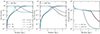 |
Fig. A.1. Expanding HII region in a pure hydrogen medium for 643 (red), 1283 (green), and 2563 (blue) gas particles. The three panels show the ion fractions at t = 100 Myr (left), t = 1500 Myr (middle) and the temperature after 100 and 1500 Myr (dashed and solid line, respectively). |
Appendix B: The impact of cell-averaged tree-based RT
Wadsley et al. (2024) showed, in idealised tests, how linearly averaging absorption in tree cells can lead to significant errors, especially when these are vastly different, as is typical for a clumpy medium. A small amount of highly opaque material can lead to an unrepresentative high opacity in a tree cell.
Neutral and ionised mass and fraction of H and He within the simulation box of MUGS2 g1536 at redshift 2.0.
Neutral and ionised mass and fraction of H and He of the most massive progenitor of MUGS2 g1536 at redshift 2.0.
In order to assess the impact of tree-based RT with cell averaged transmission in an astrophysically interesting case we performed two additional post-processing runs of MUGS2 g1536 at z = 2.0 using the original version of TREVR (Grond et al. 2019). The first run TREVR_noRef used default settings and no refinement. The second run TREVR_ref1 enforces refinement of tree cells once their optical depth exceeds a set threshold of τref = 1.0. We refer to Grond et al. (2019) for details of the refinement process in TREVR. We consider the results of the TREVR_ref1 as the most accurate and thus as reference run for this comparison.
To quantify the impact of the different methods we choose to compare the mass of ionised H and He after 300 RT post-processing steps, due to the high computational costs of TREVR with refinement. At this stage the neutral and ionised H and He masses have converged to within 10% of the final equilibrium value. Table B.1 and B.2 list the neutral and ionised H and He mass and their fraction within the whole simulation box and the most massive progenitor halo of MUGS2 g1536, respectively.
Overall the three runs are in excellent agreement with each other. On the simulation box scale the total mass of the neutral and ionised species only differ by a few percent between the three runs, considering the mass fraction the maximal difference is only 0.3%. Within the most massive progenitor halo the neutral and ionised fractions of H are within ≈1% of the reference run (TREVR_ref1), while the He fractions are with ≈0.1% of each other. Despite on a low level, there is a trend observable in these data, TREVR_noRef produces the least amount of neutral gas and TREVR2 has consistently the highest neutral fraction. We illustrate the similarities between the reference run TREVR_ref1 and TREVR2 in Fig. B.1, where we show neutral hydrogen column density (NHI).
This behaviour shows how well suited TREVR2 with transmission averaging is for zoom-in simulations of galaxies, it produces near identical ionised and neutral masses while being up to 100 times faster than TREVR with refinement.
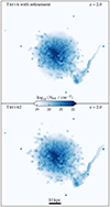 |
Fig. B.1. Face-on projected hydrogen density (NHI) of the reference run TREVR_ref1 (top) and TREVR2 with default settings (bottom) after 300 RT steps. |
All Tables
Piece-wise power-law series fit parameters (βi, j, Si, j, and Ti, j) for the approximated photo-ionisation cross-sections σ in cm2 for HI, HeI, and HeII ionisation in the considered energy bands.
Neutral and ionised H and He mass of the most massive progenitor of MUGS2 g1536 at various redshifts before and after RT post-processing.
Neutral and ionised mass and fraction of H and He within the simulation box of MUGS2 g1536 at redshift 2.0.
Neutral and ionised mass and fraction of H and He of the most massive progenitor of MUGS2 g1536 at redshift 2.0.
All Figures
|
Fig. 1. Piece-wise power-law fits to the HI, HeI, and HeII photo-ionisation cross-section (top panels) and the associated relative error (lower panels). The black dotted line shows the cross-sections from Verner et al. (1996), the blue dashed lines a simple power-law fit, and the red solid lines a power-law series (Eq. 5). The horizontal dotted lines in the lower panels indicate relative errors of 1% and 10%. |
| In the text | |
|
Fig. 2. Synthetic stellar population spectra between 1 and 200 eV for different population ages. The spectra are calculated with STARBURST99 (Leitherer et al. 2014) using the Padova AGB evolution tracks with solar metallicity and Kroupa (2001) IMF. The black line shows the PWPL reconstructed spectrum for a population age of 10 Myr. |
| In the text | |
|
Fig. 3. Haardt & Madau (2012) UV background spectrum between 1 and 1000 eV for various redshifts ranging from z = 15.1 to 0.0. The black line shows the PWPL reconstructed spectrum at z = 3. |
| In the text | |
|
Fig. 4. Photo-ionisation rate (top) and photo-heating rate (bottom), for a redshift dependent uniform Haardt & Madau (2012) UVB spectrum (left) and an aging SSP with Mcl = 106 M⊙ at a distance of 100 pc (right). The blue line shows the ionisation and heating rate for the common PWC approximation of the radiation field in combination with a constant σeff. The red line corresponds to our new PWPL approximation for the radiation field in combination with the power-law photo-ionisation cross-section (Eq. 6). |
| In the text | |
|
Fig. 5. Relative error distribution for the ionisation (top) and heating (bottom) rates, for the PWPL (reds) and PWC (blues) approximation. The left panel corresponds to the redshift dependent UVB spectrum and the right panel to the age dependent SSP spectrum for population ages below 8 Myr. Different line styles show the error distribution for HI (solid), HeI (dashed), and HeII (dot-dashed). The errors are calculated relative to the numerical integration of Eqs. (1) and (2). |
| In the text | |
|
Fig. 6. Reconstructed radiation field after t = 1500 Myr, at column densities of NHI = 1017, 1018, and 5 × 1018 cm−2 (from left to right) from the source, for the pure hydrogen (top) and primordial hydrogen and helium mixture (bottom) case. The black line denotes the CLOUDY reference runs, the red lines show the reconstructed spectrum using the PWPL approximation and the blue line represents the classic three-band PWC approach. For illustrative purposes, we represent the spectral shape of the three-band PWC case as scaled intervals of the initial black-body spectrum, while in practice it is treated as a delta function at the effective frequency of each band. |
| In the text | |
|
Fig. 7. Expanding HII region in a pure hydrogen environment with nH = 10−3 cm−3 and an initial temperature of 100 K. The hydrogen ion fractions (HI solid and HII dashed lines) after t = 100 (1500) Myr is shown in the left (middle) panel. Red lines show the results using the ten-band PWPL, blue lines using the three-band PWC approximation, and the black lines represent the CLOUDY equilibrium solution. The thin dashed line represents an ion fraction of 50%. The right panel shows the temperature profile of the HII region after t = 100 and 1500 Myr as dashed and solid lines, respectively. |
| In the text | |
|
Fig. 8. Expanding HII region in a primodial mixture of hydrogen and helium environment with nH = 10−3 cm−3 and an initial temperature of 100 K. The hydrogen ion fractions (HI solid and HII dashed lines) after t = 1500 Myr is shown in the left panel. The right panel shows the helium ion fractions (HeI solid, HeII dashed, and HeIII dotted lines) after t = 1500 Myr. The thin dashed line represents an ion fraction of 50%. |
| In the text | |
|
Fig. 9. Uniform background test. Left: Illustration of the distribution of background sources within the simulation box for 128 background emitters. The virtual background emitters are distributed along a spiral on a sphere centred on the centre of the simulation box; the point size corresponds to the distance from the viewer. Right: Incident radiation field at 13.6+ eV (HI-low) as experienced by gas particles in the uniform background test in a thin slice through the centre of the simulation box for the Haardt & Madau (2012) UVB at redshift 0 and 128 background sources. The dashed, dot-dashed, and dotted circles indicate where the radiation field is within 10%, 25%, and 50% of the expected central flux, respectively. The corresponding radii are, from the centre out, [0.26, 0.36, 0.43]×Lbox. |
| In the text | |
|
Fig. 10. Density-temperature phase-space of the most massive progenitor of g1536 at redshift 6, 2, and 0.1 (from top to bottom). The left panels show the original distribution (i.e. the initial condition for the post-processing run and the right panels show the distribution after the post-processing). The horizontal segregation at T = 2 × 10⁴ K, is artificial due to disabling of cooling for high temperature gas (see text for details). |
| In the text | |
|
Fig. 11. Location of photo-ionised gas in g1536 at z = 0.1 overlaid onto a mock i-, v-, and b-band composite image of the stellar component, viewed face on. The luminosity of the stars are calculated using Marigo et al. (2008) stellar populations, the effect of dust extinction is not included. Particles constituting the illustrated HII regions have fHII > 80%, ρ ≥ 1 cm−3 and 7 × 10³ ≤ T/K ≤ 3 × 10⁴. |
| In the text | |
|
Fig. 12. Ion mass relative to the initial ion mass before RT post-processing, for the considered species of the chemical network, of the most massive progenitor of g1536 at various redshifts. |
| In the text | |
|
Fig. 13. Face-on projection of the neutral hydrogen density (NHI) in a region with 100 kpc per side centred on the most massive progenitor of g1536 at z = 2 before (left) and after (right) RT post-processing. |
| In the text | |
|
Fig. 14. Face-on projected total gas density (Σgas) in a region with 100 kpc per side centred on the most massive progenitor of g1536 at z = 2. |
| In the text | |
|
Fig. A.1. Expanding HII region in a pure hydrogen medium for 643 (red), 1283 (green), and 2563 (blue) gas particles. The three panels show the ion fractions at t = 100 Myr (left), t = 1500 Myr (middle) and the temperature after 100 and 1500 Myr (dashed and solid line, respectively). |
| In the text | |
|
Fig. B.1. Face-on projected hydrogen density (NHI) of the reference run TREVR_ref1 (top) and TREVR2 with default settings (bottom) after 300 RT steps. |
| In the text | |
Current usage metrics show cumulative count of Article Views (full-text article views including HTML views, PDF and ePub downloads, according to the available data) and Abstracts Views on Vision4Press platform.
Data correspond to usage on the plateform after 2015. The current usage metrics is available 48-96 hours after online publication and is updated daily on week days.
Initial download of the metrics may take a while.