| Issue |
A&A
Volume 690, October 2024
|
|
|---|---|---|
| Article Number | A225 | |
| Number of page(s) | 19 | |
| Section | Interstellar and circumstellar matter | |
| DOI | https://doi.org/10.1051/0004-6361/202451065 | |
| Published online | 10 October 2024 | |
Evidence for magnetic boundary layer accretion in RU Lup
A spectrophotometric analysis★
1
Institut für Astronomie und Astrophysik, Eberhard Karls Universität Tübingen,
Sand 1,
72076
Tübingen,
Germany
2
INAF – Osservatorio Astrofisico di Catania,
via S. Sofia 78,
95123
Catania,
Italy
3
European Southern Observatory,
Karl-Schwarzschild-Strasse 2,
85748
Garching bei München,
Germany
4
Department of Physics & Astronomy, Stony Brook University,
Stony Brook,
NY,
11794-3800,
USA
5
INAF – Osservatorio Astronomico di Capodimonte,
via Moiariello 16,
80131
Napoli,
Italy
6
Hamburger Sternwarte,
Gojenbergsweg 112,
21029
Hamburg,
Germany
7
SUPA, School of Science and Engineering, University of Dundee, Nethergate,
DD1 4HN,
Dundee,
UK
8
Instituto de Astrofísica e Ciências do Espaço, Universidade do Porto, CAUP, Rua das Estrelas,
4150-762
Porto,
Portugal
9
Departamento de Física e Astronomia, Faculdade de Ciências, Universidade do Porto,
Rua do Campo Alegre 687,
4169-007
Porto,
Portugal
10
INAF – Osservatorio Astronomico di Roma,
via Frascati 33,
00078
Monte Porzio Catone,
Italy
11
ASI, Italian Space Agency, via del Politecnico snc,
00133
Rome,
Italy
★★ Corresponding author; This email address is being protected from spambots. You need JavaScript enabled to view it.
Received:
11
June
2024
Accepted:
9
August
2024
Abstract
Context. It is well established that classical T Tauri stars accrete material from a circumstellar disk through magnetic fields. However, the physics regulating the processes in the inner (0.1 AU) disk is still not well understood.
Aims. Our aim is to characterize the accretion process of the classical T Tauri Star RU Lup.
Methods. Optical high-resolution spectroscopic observations with CHIRON and ESPRESSO were obtained simultaneously with photometric data from AAVSO and TESS.
Results. We detected a periodic modulation in the narrow component of the He I 5876 line with a period that is compatible with the stellar rotation period, indicating the presence of a compact region on the stellar surface that we identified as the footprint of the accretion shock. We show that this region is responsible for the veiling spectrum, which is made up of a continuum component plus narrow line emission that fills in the photospheric lines. An analysis of the high-cadence TESS light curve reveals quasi-periodic oscillations on timescales shorter than the stellar rotation period, suggesting that the accretion disk in RU Lup extends inward of the corotation radius, with a truncation radius at ~2 R*. This is compatible with predictions from three-dimensional magnetohydrodynamic models of accretion through a magnetic boundary layer (MBL). In this scenario, the photometric variability of RU Lup is produced by a nonsta-tionary hot spot on the stellar surface that rotates with the Keplerian period at the truncation radius. We also qualitatively discuss how more complex hot spot shapes may generate the same variability pattern. The analysis of the broad components of selected emission lines reveals the existence of a non-axisymmetric, temperature-stratified flow around the star, in which the gas leaves the accretion disk at the truncation radius and accretes onto the star channeled by the magnetic field lines. The unusually rich metallic emission line spectrum of RU Lup might be characteristic of the MBL regime of accretion.
Conclusions. Our extensive multiwavelength database of RU Lup reveals many similarities to predictions from the scenario of accretion through a magnetic boundary layer. Alternative explanations would require the existence of a hot spot with a complex shape, perhaps made of two brighter knots, or a warped structure in the inner disk.
Key words: accretion, accretion disks / stars: individual: RU Lup / stars: pre-main sequence / stars: variables: T Tauri, Herbig Ae/Be
Based on observations collected at the European Southern Observatory under ESO programs 106.20Z8.003 and 106.20Z8.007.
© The Authors 2024
 Open Access article, published by EDP Sciences, under the terms of the Creative Commons Attribution License (https://creativecommons.org/licenses/by/4.0), which permits unrestricted use, distribution, and reproduction in any medium, provided the original work is properly cited.
This article is published in open access under the Subscribe to Open model. This email address is being protected from spambots. You need JavaScript enabled to view it. to support open access publication.
1 Introduction
Classical T Tauri stars (CTTSs) are young (~1–10 Myr), low-mass (<2 M⊙) objects that accrete material from a circumstellar disk (Hartmann et al. 2016). Their strong magnetic fields truncate the disk at a few stellar radii (typically 5 R*, Hartmann et al. 2016). The current paradigm for the interaction between the disk and the star is magnetospheric accretion (Bouvier et al. 2007b), in which the material free-falls onto the star following the magnetic field lines.
The rich emission line spectrum is one of the defining characteristics of these systems (Joy 1945; Herbig 1962). The optical spectrum of CTTSs displays strong and broad (with a full width at zero intensity ≳200 km s−1) permitted emission lines, such as the Balmer, He I, and Ca II H & K lines. Sometimes other metallic species such as Na I, Mg I, Ca I, Ca II, Fe I, and Fe II are observed in emission, especially during epochs of an increased accretion rate (e.g., Sicilia-Aguilar et al. 2012; Armeni et al. 2023). Permitted lines are thought to be formed in different structures around the star. The observed supersonic velocities, roughly consistent with free-fall velocities, suggest that the broad component (BC) of permitted emission lines is formed in the magnetospheric accretion flow (Hartmann et al. 2016). Many studies have shown that the Balmer and other emission line profiles and variability are compatible with this scenario (e.g., Muzerolle et al. 1998; Alencar et al. 2012; Bouvier et al. 2007a) and that their luminosity is related to the accretion rate of the system (Alcalá et al. 2017). The helium and metallic lines are also useful tracers of the dynamics of the accretion flow (Beristain et al. 1998, 2001). These lines typically show a narrow component (NC) superposed on the BC. The NC is formed in the footprint of the magnetic field on the stellar surface – that is, the post-shock region – and it is rotationally modulated with the stellar rotation period (Sicilia-Aguilar et al. 2015; Campbell-White et al. 2021). The different behavior between the BC of the He I and metallic lines and their different excitation conditions suggest the presence of temperature and density gradients in the accretion flow (Armeni et al. 2023). In particular, the He I lines require high-energy conditions that can be achieved in the preshock region, which is irradiated by the X-rays from the shock (Hartmann et al. 2016). Under such conditions, species such as Na, Ca, and Fe are expected to be highly ionized. For this reason, the low-ionized metallic lines are thought to originate closer to the disk (Sicilia-Aguilar et al. 2012, 2023; Armeni et al. 2023), where the dilution factor of the radiation from the shock is lower (Azevedo et al. 2006).
Another observational feature in the optical spectrum of CTTSs is the presence of a continuum excess flux relative to the photospheric spectrum, which results from the accretion shock at the stellar surface (Calvet & Gullbring 1998). This excess makes the photospheric absorption lines appear less deep in normalized spectra, an effect known as veiling (Hartigan et al. 1989). The veiling fraction (VF) is defined as the ratio of the excess flux, Facc, due to accretion relative to the photo-spheric flux, Fphot; that is, VFλ = Facc(λ)/Fphot(λ). Gahm et al. (2008) showed that for extremely veiled (VF ≳ 2) CTTSs another component contributes to the veiling: line filling emission in the absorption lines, which dilutes the photospheric spectrum without any changes in the continuum emission from shocked regions.
Three-dimensional (3D) magnetohydrodynamic (MHD) simulations showed that the interaction between the star and the disk is complex (Romanova & Owocki 2015). It has been shown that CTTSs may accrete in either a stable or an unstable regime (Romanova et al. 2003, 2004; Kulkarni & Romanova 2008; Pantolmos et al. 2020). In the stable regime, the disk matter is channeled in funnel streams by the magnetic fields, forming polar hot spots on the stellar surface. In the Rayleigh-Taylor (RT) unstable regime, the matter penetrates through the magnetosphere in tongues. This leads to the formation of several chaotic hot spots close to the stellar equator. The light curves are expected to be periodic with the stellar rotation period (P*) in the stable regime and stochastic in the unstable regime.
According to the simulations, the transition between the stable and unstable regimes depends on the ratio between the magnetospheric truncation radius, RT, and the corotation radius, Rco. The corotation radius is the radius at which the Keplerian angular velocity of the disk matches the angular velocity of the star. The truncation radius is defined as the radius where the magnetic field pressure is equal to the ram pressure in the disk. By fitting the results of a series of 3D MHD simulations, Kulkarni & Romanova (2013) showed that
![Mathematical equation: $\[\frac{R_{\mathrm{T}}}{R_{\star}}=1.06\left(\frac{B_{\star}^4 R_{\star}^5}{\dot{M}_{\mathrm{acc}}^2 G M_{\star}}\right)^{1 / 10},\]$](/articles/aa/full_html/2024/10/aa51065-24/aa51065-24-eq1.png) (1)
(1)
where R* is the stellar radius, B* is the strength of the stellar dipolar magnetic field at the stellar surface, ![Mathematical equation: $\[\dot{M}_{\mathrm{acc}}\]$](/articles/aa/full_html/2024/10/aa51065-24/aa51065-24-eq2.png) is the mass accretion rate from the disk, G is the gravitational constant, and M* is the stellar mass. All parameters are in cgs units. Accretion is unstable if RT/Rco ≲ 0.71 and stable otherwise (Blinova et al. 2016).
is the mass accretion rate from the disk, G is the gravitational constant, and M* is the stellar mass. All parameters are in cgs units. Accretion is unstable if RT/Rco ≲ 0.71 and stable otherwise (Blinova et al. 2016).
Romanova & Kulkarni (2009) showed that in systems with small magnetospheres, unstable accretion proceeds through a magnetic boundary layer (MBL). In this regime, two ordered streams are formed. These tongues of matter and the resulting hot spots rotate with the Keplerian period, PT, at the truncation radius. This leads to the observation of quasi-periodic oscillations (QPOs) at PT in the light curves. In their simulations, the authors observed a correlation between the size of the magnetosphere and the period of the QPOs. When the magnetosphere is smaller, the detected period decreases. Blinova et al. (2016) further investigated the conditions for the development of this regime, showing that it occurs for systems with RT ≲ 4.2 R* when RT/Rco ≲ 0.59.
This work focuses on RU Lup (Sz 83), a young K7 star (Alcalá et al. 2017) located in the Lupus cloud at a distance of 158.9 ± 0.7 pc (Gaia Collaboration 2021). RU Lup is a monitoring target within the Hubble UV Legacy Library of Young Stars as Essential Standards, (ULLYSES, Roman-Duval et al. 2020; Espaillat et al. 2022) survey for CTTSs. Manara et al. (2023) reported a value of ![Mathematical equation: $\[\dot{M}_{\mathrm{acc}}\]$](/articles/aa/full_html/2024/10/aa51065-24/aa51065-24-eq3.png) = 10−7 M⊙ yr−1 for RU Lup, making it the strongest accretor in Lupus. This star is also very active, with an accretion rate that can vary up to a factor of 2 on a timescale of weeks (Stock et al. 2022). Wendeborn et al. (2024a) show that the accretion rate reached median values of 1.7 × 10⁻⁷ M⊙ yr−1 in 2021, and it dropped considerably one year later, with a median of 6 ×10⁻⁸ M⊙ yr−1. Stempels et al. (2007) derived P* = 3.71 d by analyzing the radial velocity of the photospheric absorption lines. Many works have focused on the photometric variability of RU Lup, but failed to recover any stable periodicity (Percy et al. 2010; Siwak et al. 2016; Wendeborn et al. 2024b).
= 10−7 M⊙ yr−1 for RU Lup, making it the strongest accretor in Lupus. This star is also very active, with an accretion rate that can vary up to a factor of 2 on a timescale of weeks (Stock et al. 2022). Wendeborn et al. (2024a) show that the accretion rate reached median values of 1.7 × 10⁻⁷ M⊙ yr−1 in 2021, and it dropped considerably one year later, with a median of 6 ×10⁻⁸ M⊙ yr−1. Stempels et al. (2007) derived P* = 3.71 d by analyzing the radial velocity of the photospheric absorption lines. Many works have focused on the photometric variability of RU Lup, but failed to recover any stable periodicity (Percy et al. 2010; Siwak et al. 2016; Wendeborn et al. 2024b).
Herczeg et al. (2005) estimated Av ~ 0.07 mag for RU Lup. This value is compatible with its pole-on orientation, obtained from both spectroscopy (Stempels et al. 2007) and interferometry (GRAVITY Collaboration 2021). This allows us to study the accretion process and its variability without the contribution of variable extinction due to circumstellar dust in our line of sight. The optical spectrum of RU Lup comprises a plethora of emission lines from metallic species.
These characteristics make RU Lup suitable for studying the magnetospheric accretion process in a likely RT-unstable regime (given its high ![Mathematical equation: $\[\dot{M}_{\mathrm{acc}}\]$](/articles/aa/full_html/2024/10/aa51065-24/aa51065-24-eq4.png) , Stock et al. 2022) by comparing photometric observations with 3D MHD simulations. The spectroscopic data allows instead to study the star-disk interaction and the physics regulating the processes in the inner, gaseous disk.
, Stock et al. 2022) by comparing photometric observations with 3D MHD simulations. The spectroscopic data allows instead to study the star-disk interaction and the physics regulating the processes in the inner, gaseous disk.
This paper is organized as follows. In Sect. 2, we present the observations. We update the stellar parameters of RU Lup in Sec. 3. We present the analysis of the NCs and the veiling spectrum in Sec. 4, the analysis of the BC of the metallic lines in Sec. 5, and the analysis of the TESS light curve in Sec. 6. We discuss the results in Sec. 7 and outline our conclusions in Sec. 8.
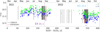 |
Fig. 1 AAVSO B (blue) and V (green) photometry contemporaneous to the spectroscopic observations in 2021 and 2022. The vertical dashed lines mark the epochs of the CHIRON (black) and ESPRESSO (red) observations. The ES 21.1 and ES 22.5 spectra shown in Fig. 2 are marked in violet and light blue. Here, MJD0 ≡ 59264.336. |
2 Observations
In this section, we describe the data that we used to study RU Lup.
2.1 Spectroscopy
The spectroscopic data were obtained with two different instruments. Medium-resolution optical (4080–8900 Å) spectra were obtained with CHIRON (Tokovinin et al. 2013), an echelle spectrograph mounted on a 1.5 m telescope that is part of the Small and Moderate Aperture Research Telescope System (SMARTS) at Cerro Tololo Inter-American Observatory. A total of 58 spectra were taken in three different epochs: 19 spectra in 2021, 27 spectra in 2022, and 12 spectra in 2023. Except for three observations taken at a resolving power of R = 78 000 in 2021, the rest of the CHIRON observations have R = 27 800. The spectra were reduced and flux-calibrated in the manner described by Walter (2018)1.
High-resolution (R = 140 000) optical (3800–7880 Å) spectra were obtained with the Echelle SPectrograph for Rocky Exoplanets and Stable Spectroscopic Observations (ESPRESSO, Pepe et al. 2021) in the framework of the PENELLOPE program (Manara et al. 2021). Two spectra were obtained in 2021 in Pr. ID 106.20Z8.003 and five in 2022 in Pr. ID 106.20Z8.007 (PI Manara). The ESPRESSO spectra were reduced by the PENELLOPE team, as is described in Manara et al. (2021). Telluric correction was performed using the molecfit tool (Smette et al. 2015).
For clarity, throughout this article each spectrum is labeled as “ID yy.j” where ID is either CH or ES for a CHIRON or ESPRESSO observation, respectively, yy are the last two digits of the year, and j is the jth observation from that spectrograph in that year. For example, the third ESPRESSO observation from 2022 is called ES 22.3. The log of the spectroscopic observations is reported in Table A.1.
2.2 Photometry
RU Lup was observed with the Transiting Exoplanet Survey Satellite (TESS, Ricker et al. 2014). TESS produces short-cadence, about one-month-long light curves with a spectral response that covers the red/infrared wavelength range (~0.6–1.1 μm). The observation is a 200 seconds cadence light curve from Sector 65 (2023). We downloaded the light curve, extracted and reduced by the TESS Science Processing Operations Center (SPOC), from the MAST archive2. The TESS Sector 65 light curve is contemporaneous to nine CHIRON observations from 2023.
To supplement the spectroscopic observations with multiband photometry, we downloaded data from the American Association of Variable Star Observers (AAVSO) International Database3. This data set is composed of BVRcIc photometry taken in 2021 and 2022. For spectroscopic data that were taken close in time to a set of photometric observations, we used the B, V, Rc photometry to flux-calibrate the spectra, following the procedure outlined by Armeni et al. (2023). We set an upper limit of 0.25 days (6 hours) on the temporal distance between the spectrum and the photometry, based on the photometric variability of the system inferred from TESS (Sec. 6). Figure 1 shows the AAVSO B and V photometry, together with the spectroscopic observations from 2021 and 2022.
In summary, we have three different epochs of spectroscopic observations: 2021, 2022, and 2023. The first two are supplemented by the AAVSO photometry, while the last one by the TESS Sector 65 light curve.
3 Stellar parameters with ESPRESSO
The photospheric parameters of RU Lup were previously estimated by Frasca et al. (2017) by fitting a medium-resolution (R ~ 17400) X-Shooter (Vernet et al. 2011) spectrum with the ROTFIT routine (Frasca et al. 2015). Here, we take advantage of the higher resolution of the ESPRESSO spectra to improve these measurements.
Fitting a spectrum of a highly accreting CTTS such as RU Lup is not an easy task. In some epochs, the spectrum is dominated by broad emission lines that make it difficult to identify the continuum. In addition, the photospheric lines are weaker because of veiling. An example of such an extreme veiling state is the ES 21.1 observation, shown in Fig. 2 in violet. The region between 5770 and 5805 Å shows the effect of line-filling emission of the photospheric lines. The multi-epoch monitoring of RU Lup with ESPRESSO allowed us to observe the system in a state of lower veiling with a signal-to-noise ratio (S/N) of ~40. This observation (ES 22.5) is shown in Fig. 2 in light blue. We focused on this spectrum to determine the stellar parameters.
We applied ROTFIT to different portions of the spectrum, masking emission lines where necessary. We used as templates a library of High Accuracy Radial velocity Planet Searcher (HARPS, Mayor et al. 2003) spectra of real stars retrieved from the ESO Archive (see Manara et al. 2021). This library is mostly composed of main-sequence stars, with the exception of the early-K spectral type for which subgiant stars are also included. We avoided including weak-lined T Tauri stars because for most of them the projected rotational velocities are too high for the fitting purposes. Moreover, some of their lines are contaminated by strong chromospheric emission. Since the templates are more evolved than our targets, the values of log g determined with these templates can be overestimated. For this reason we do not report here the log g measured for RU Lup. The stellar parameters obtained from the ROTFIT analysis of the ESPRESSO spectra are reported in Table 1, together with the other properties of RU Lup adopted from the literature. Thanks to the high resolution of ESPRESSO, we improved the measurement of the projected stellar rotational velocity (v sin i), reducing the uncertainty by a factor of ~3.5 relative to the uncertainty given by Frasca et al. (2017).
Using the stellar luminosity (L*) obtained by Manara et al. (2023), we computed the stellar radius by inverting the Stefan-Boltzmann law ![Mathematical equation: $\[L_{\star}=4 \pi R_{\star}^2 \sigma T_{\text {eff }}^4\]$](/articles/aa/full_html/2024/10/aa51065-24/aa51065-24-eq6.png) . The estimate of the stellar mass (M*) from Manara et al. (2023), together with P* (Stempels et al. 2007) results in Rco = 8.26 ± 0.65 R⊙ = 3.64 ± 0.88 R*.
. The estimate of the stellar mass (M*) from Manara et al. (2023), together with P* (Stempels et al. 2007) results in Rco = 8.26 ± 0.65 R⊙ = 3.64 ± 0.88 R*.
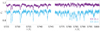 |
Fig. 2 ES 21.1 and ES 22.5 spectra in two regions where the photospheric absorption lines are observed. The region between 5770 and 5805 Å shows the effect of line-filling emission. |
Stellar parameters of RU Lup.
4 Hot spot revealed by narrow component variability
The magnetospheric accretion scenario predicts the presence of hot spots on the stellar surface. The hot spots produce an excess continuum flux (Calvet & Gullbring 1998), that can be observed photometrically (e.g., Espaillat et al. 2021), and NCs in emission lines of species such as He I, He II, Fe I, Fe II, Ca II, etc. (Dodin & Lamzin 2012) that can be traced spectroscopically (McGinnis et al. 2020). Since they are formed close to the stellar surface, the NCs are expected to be rotationally modulated with P*. The radial velocity of the NC describes a sinusoidal curve as the star rotates
![Mathematical equation: $\[v_{\mathrm{rad}}(\phi)=v_0+v \sin i \cdot \cos \theta_{\mathrm{S}} \cdot \sin \left[2 \pi\left(\phi-\phi_{\mathrm{S}}\right)\right]\]$](/articles/aa/full_html/2024/10/aa51065-24/aa51065-24-eq7.png) (2)
(2)
(e.g., Sicilia-Aguilar et al. 2015; McGinnis et al. 2020). Here, v0 is an offset velocity that includes the stellar systemic velocity and any other velocities due to additional motions of the emitting material (such as infall), ϕ and ϕS are phase angles (0 ≤ ϕ, ϕS < 1), and θS is the latitude of the spot; that is, the angle between the position of the spot and the stellar equator. The amplitude A = v sin i · cos θS of the modulation is, thus, a fraction of v sin i and the closer the spot is to the pole, the smaller the modulation.
The study of the NC variability in EX Lup and TW Hya (Campbell-White et al. 2021; Sicilia-Aguilar et al. 2023) showed how lines from different species exhibit different amplitudes and phases, and hence trace material at different positions on the stellar surface. These studies also revealed that these line-emitting regions are surprisingly stable over several years, even when the accretion rate increases (e.g., during the bursts of EX Lup, Sicilia-Aguilar et al. 2023). In our case, the study of the NCs is limited by the spectral resolution of the observations. The NC of the metallic lines is typically narrower than, for instance, the NC of the He I lines, making it difficult to detect in the lower resolution CHIRON spectra. Moreover, strong line blends (e.g., between the He I 5016 and Fe II 5018 lines) and contamination by photospheric absorption lines (e.g., in the He II 4686 line) complicate the fit of the NC. For these reasons, we focused on the He I 5876 line, the NC of which can always be discerned in our spectra.
4.1 Modulation of the He I 5876 narrow component
The usual approach is to fit the line profile with two Gaussian functions, one for the BC and one for the NC (e.g., Campbell-White et al. 2021). However, the He I 5876 line profiles of RU Lup are more complex and we had to modify the fit function (see Appendix B). We used three Gaussian functions, two accounting for the BC and one for the NC. In addition, we allowed the Gaussian for the NC to be asymmetric, with two different widths (parameterized by the standard deviation, σ), one for the red wing (σr) and the other for the blue wing (σb). Figure 3 displays the best fit of the He I 5876 line for the ES 21.1 spectrum with two different models, one using three symmetric Gaussian functions (3S) and one using the asymmetric Gaussian for the NC (2S+1A). The 2S+1A best fit demonstrates that the NC red wing is more extended than the blue wing, with σr = 32.9 ± 0.5 km s−1 and σb = 14.9 ± 0.4 km s−1. This is in agreement with formation in an infalling region. The comparison between the chi-square (χ2) of the two models indicates that the 2S+1A model better reproduces the line profile.
We fit our observations with the 2S+1A model and obtained the radial velocity of the NC (vNC), defined as in Eq. (B.1), as a function of time. Then, we computed the Lomb-Scargle Periodogram (LSP, Lomb 1976; Scargle 1982) of these radial velocity measurements. The result is shown in Fig. 4. We detected a signal with a false alarm probabilty (FAP) of 0.2% at a period of 3.63 days, that differs by ~2 h from the stellar rotation period presented by Stempels et al. (2007). The discrepancy with the Stempels et al. (2007) period can be attributed to the intrinsic variability of the region that is traced by the NC.
Figure 5 shows the radial velocity curve, phase-folded using the detected period and MJD0 ≡ 59264.336 as reference date for ϕ = 0. Although there is a ~1 km s−1 variability between different epochs and some outliers (e.g, at ϕ ≈ 0.6) the modulation is overall sinusoidal. The best fit of the radial velocity curve with a sinusoidal function (Eq. (2)) gives information about the position of the emitting region on the stellar surface (Sicilia-Aguilar et al. 2015). We obtained v0 = 1.46 ± 0.09 km s−1, A = 2.53 ± 0.13 km s−1, and ϕS = 0.75 ± 0.01. Using v sin i = 8.6 ± 1.4 km s−1 (Sec. 3), we derived θS = 73 ± 3 °. The magnetic obliquity Θ = 90° – θS, that is, the angle between the stellar rotation axis and the position of the NC-emitting region (McGinnis et al. 2020), is ~20°, indicating that the magnetic field axis is misaligned with respect to the stellar rotation axis. The footprint of the magnetic field is close to the stellar pole, similar to what is observed for EX Lup and TW Hya (Sicilia-Aguilar et al. 2023).
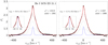 |
Fig. 3 Best fit of the He I 5876 line in ES 21.1 with two different models. Both models use three Gaussian functions. In the left panel, the Gaussian for the NC is symmetric, while in the right panel it has two different σ. See Appendix B for details on the model. The single components are marked with dashed lines, with the blue one indicating the Gaussian for the NC. The insets are a zoom on the NC. |
 |
Fig. 4 Lomb Scargle Periodogram of the radial velocity of the He I 5876 NC. |
4.2 Narrow component of the helium and metallic lines
Although the resolution and the S/N of the CHIRON spectra did not allow us to study the modulation of the NC of the metallic lines, these components can be discerned in the ESPRESSO spectra with high S/N. We selected six emission lines that show a NC in ES 22.5, namely the He I 5876, He II 4686, Mg I 5184, Si II 6347, Fe I 5447, and Fe II 5317 lines. The profile of some of these lines is severely contaminated by the underlying photospheric absorption. Therefore, we used our best fit non-accreting template to remove the stellar contribution. For each line, we adjusted the veiling to match the depth of the photospheric lines. This procedure worked for all but the Fe II 5317 line, for which the photospheric HARPS template has a gap. However, the line is strong enough that its profile can be fit even without removing the photospheric spectrum.
We fit the photospheric subtracted spectra with the multiple Gaussian model introduced in Sec. 4.1, with the aim of deriving the parameters of the NC. For all lines, an asymmetric Gaussian was used to fit the NC. The results are illustrated in Fig. 6. The red asymmetry already observed in the He I 5876 NC appears to be a common feature of the NCs of the metallic lines, with the higher-excitation lines (i.e., Si II and Fe II) being more asymmetric. Conversely, the He II line appears to be symmetric. The NCs of the helium lines are substantially broader than those of the metallic lines, suggesting that these two sets of NCs are formed in different regions of the hot spot structure. This is in agreement with the energy requirements for the formation of the helium lines. Since the upper level of the He II 4686 line has Ej = 51.01 eV, this line must be formed in a region that is irradiated by the X-rays from the accretion shock. Under such conditions, magnesium and iron are expected to be ionized at least once.
4.3 Anti-phase radial velocity variations
We calculated the photospheric velocity relative to the ES 22.5 spectrum, vphot, by cross-correlating the latter with the other ESPRESSO spectra in the region between 5725 and 5745 Å. Figure 7 shows how vphot is in anti-phase with vNC. This effect was already observed for RW Aur (Petrov et al. 2001), DR Tau (Petrov et al. 2011), and EX Lup (Sicilia-Aguilar et al. 2015), and can be explained with the rotation of a hot spot that emits in narrow emission lines and distorts the photospheric absorption lines. This feature is offset relative to the stellar rotation axis, producing a rotational modulation of the centroids of both emission and absorption lines, which are in anti-phase (e.g., Petrov et al. 2011; Rei et al. 2018). Therefore, the anti-phase radial velocity variations of the He I 5876 NC and the photospheric lines confirms the hypothesis that the NCs are produced in a hot spot on the stellar surface in RU Lup.
4.4 Veiling spectrum: Continuum and line emission
We focused on the high-resolution ESPRESSO spectra to study the veiling spectrum. Figure 2 shows how the photospheric lines are not only veiled by an excess continuum, but also by narrow line-filling emission likely coming from the hot spot (Sec. 4.3).
Since the ESPRESSO spectra are absolutely flux-calibrated, it is possible to disentangle the continuum and the line emission contribution to the veiling. To do this, we subtracted ES 22.5 from the other ESPRESSO observations, after correcting for shifts in radial velocity by cross-correlating the spectra. This procedure is a flux-calibrated version of the one employed by Herczeg et al. (2023) to measure the veiling in TW Hya. The result is illustrated in Fig. 8 for the region around 5800 Å.
Under the assumption that the ES 22.5 observation represents the photospheric spectrum plus a featureless continuum with a VF of VFT = 1.57 (Sec. 3), the subtraction removes the photospheric spectrum and reveals the veiling spectrum, which consists of two components: continuum and line emission. The continuum veiling fraction relative to ES 22.5 (VFC) can be directly calculated as the ratio between the average fluxes of the subtracted spectrum and the ES 22.5 spectrum in the region between 5800 and 5803 Å, where the spectra are free of absorption lines. This means that in the subtracted spectra, that region represents the excess continuum relative to ES 22.5.
In Appendix C, we calculated the relative veiling, VFrel, between any given spectrum and the template ES 22.5 by finding the value that best fits the normalized spectrum assuming that the photospheric lines are weakened only by an excess continuum. This value is much higher than the value of VFc that we find above for the same wavelength region. As an example, we calculated VFrel = 2.91 ± 0.11 and VFC = 0.52 ± 0.03 for the ES 21.1 observation. The values of VFC and VFrel are different because of the effect of line-filling emission, which reduces the depth of the photospheric lines in normalized spectra in the same way as a diluting continuum (see, e.g., Fig. C.1). This result highlights the importance of the contribution of the line-filling emission to the veiling in highly veiled CTTSs, as already discussed by Gahm et al. (2008), Petrov et al. (2011), and Rei et al. (2018).
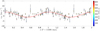 |
Fig. 5 Phase-folded radial velocity curve of the He I 5876 NC. The red line is the best fit with a sinusoidal function. |
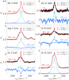 |
Fig. 6 Selection of emission lines that have a NC. The light blue spectrum is ES 22.5. The dark blue spectra are the template that best fits the stellar spectrum (Sec. 3), veiled to match the depth of the photo-spheric lines. The photospheric subtracted spectra are shown in black, with Gaussian best fits superposed in red. The red label specifies the multiple Gaussian model used (Appendix B). |
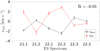 |
Fig. 7 Anti-phase radial velocity variations of the He I 5876 NC (red) and the photospheric lines (black) in the ESPRESSO spectra. R is the Pearson correlation coefficient between vphot and vNC. |
5 Spectroscopic variability of the metallic lines
The two spectra in Fig. 2 represent two different states of veiling of RU Lup. We estimated the veiling of the ES 21.1 observation, as is explained in Appendix C, obtaining VF = 5.6 ± 0.9. For the ES 22.5 spectrum, we derived VF = 1.6 ± 0.3 (Sec. 3). Figure 9 shows the differences in the emission line spectrum between these two observations. Emission lines from Fe II (e.g, Fe II 5363 and 5535) are present in both spectra, but they are stronger relative to the continuum in ES 21.1. The emission line spectrum is richer in ES 21.1, with a large number of transitions, mostly from neutral species such as Fe I and Ti I, appearing in emission. These metallic lines have a BC with a full width at half maximum (FWHM) of ~150 km s−1. In Fig. 9 we marked in red the Fe I 5447, Si II 6347, and Ca I 6122 lines, which are not blended with other lines and are clear examples of how the line strength increases relative to the continuum in the spectrum with higher veiling. The Ca I doublet (λλ 6103, 6122) has the most striking variability between the two observations, being strongly in absorption in ES 22.5 but completely filled in with emission in ES 21.1. The comparison between the ES 21.1 and 22.5 spectra indicates that the strength of these lines can be used as proxy of states of the accretion state.
Several studies (e.g., Petrov et al. 2001; Sicilia-Aguilar et al. 2012, 2023) showed that the BC of the metallic lines is formed in the circumstellar environment of the star. However, these lines must be formed in a different region with respect to, for instance, the He I lines. Iron and calcium are expected to be ionized in the high temperature conditions required for the formation of the He I lines (Armeni et al. 2023).
To understand the difference between the region of formation of these species, we selected four emission lines to analyze their BC. These lines are the He I 6678, Fe I 5447, Fe II 5317, and Si II 6347 lines. The λ5447 and λ5317 lines are among the few iron lines that are isolated and not blended with other emission lines. We chose the λ6678 line instead of the λ5876 line for He I because it is less optically thick, hence a better tracer of the gas dynamics. The Si II 6347 line was selected because its profile is not contaminated by photospheric absorption, given the high energy of its lower level (Ei = 8.12 eV). The lines are plotted in absolute flux in Fig. 10.
The comparison between the Fe II 5317 line profiles in the ESPRESSO spectra shows the existence of a component with a variable radial velocity. This is illustrated in Fig. 11, where three sets of two consecutive ESPRESSO observations are subtracted from each other in the Fe II 5317 line. Before subtracting, we rescaled the line profiles so that the wings matched. The subtraction reveals that the component has velocity centroids ranging between ~-90 and ~+35 km s−1 and it is responsible for the variations in the shape of the line.
The variability of the asymmetry of the BC suggests the presence of a non-axisymmetric structure rotating around the star. To further explore this scenario, we fit the other three selected lines with Gaussian functions. For all three lines, we used an asymmetric Gaussian to fit the BC. The NC of the He I 6678 line can be always discerned in our observations. Therefore, we fit the He I line profiles with a 1S+1A model. Conversely, the NC of the Fe I and Si II lines is sometimes absent or it cannot be discerned in observations with lower S/N. For this reason, we masked the profiles of these lines between −15 and +15 km s−1 and fit the remaining line profile with a 1A model. The fit parameters for the BCs are the strength of the component relative to the continuum (CBC), its velocity (vBC), and the widths of the blue and red wings (σb and σr). From the widths, we derived the FWHM and the line asymmetry to the blue (LA) as ![Mathematical equation: $\[\mathrm{FWHM}=\sqrt{2 \ln 2} \cdot\left(\sigma_{\mathrm{b}}+\sigma_{\mathrm{r}}\right)\]$](/articles/aa/full_html/2024/10/aa51065-24/aa51065-24-eq8.png) and LA = σb/(σb + σr). When the line was weak relative to the continuum, the fit did not converge. For this reason, we excluded fits with CBC < 0.2 for Fe I 5447 and CBC < 0.1 for Si II 6347. The results of the best fits are displayed in Fig. 12 in the form of the relation between vBC and LA for each emission line. There is a high (Pearson R > 0.70) positive correlation between these two parameters for each line, that is, the higher LA, the more the line center is redshifted. The He I 6678 BC is less influenced by line shifts, it is most of the times asymmetric to the blue (LA > 0.5) and redshifted. Also the Fe I 5547 BC is redshifted in 42 out of 53 observations, and it is sometimes highly blue-skewed (with LA ≳ 0.7). The Si II 6347 BC is the only one with significant asymmetry to the red (LA < 0. 5). All the lines have vBC between −30 and +60 km s−1.
and LA = σb/(σb + σr). When the line was weak relative to the continuum, the fit did not converge. For this reason, we excluded fits with CBC < 0.2 for Fe I 5447 and CBC < 0.1 for Si II 6347. The results of the best fits are displayed in Fig. 12 in the form of the relation between vBC and LA for each emission line. There is a high (Pearson R > 0.70) positive correlation between these two parameters for each line, that is, the higher LA, the more the line center is redshifted. The He I 6678 BC is less influenced by line shifts, it is most of the times asymmetric to the blue (LA > 0.5) and redshifted. Also the Fe I 5547 BC is redshifted in 42 out of 53 observations, and it is sometimes highly blue-skewed (with LA ≳ 0.7). The Si II 6347 BC is the only one with significant asymmetry to the red (LA < 0. 5). All the lines have vBC between −30 and +60 km s−1.
A selection of four observations that highlight the variability of the line asymmetry is shown in Fig. 13. In CH 21.10 and CH 22.7 the Si II BC is blue-skewed, while in CH 22.27 and CH 23.1 it is red-skewed. The change from red to blue asymmetry is in agreement with what is observed in the Fe II 5317 line and further supports the hypothesis of a non-axysimmetric flow rotating around the star. Different transitions have different line asymmetries in the same observation, suggesting that although these emission lines are produced in the accretion flow, they trace different regions of it. This is confirmed by the different FWHM of the lines, which is on average ~250, 190, and 173 km s−1, for the He I, Si II, and Fe I lines, respectively. These values are compatible with a formation in a stratified flow, as observed for HM Lup (Armeni et al. 2023). The He I 6678 line has the most extreme excitation conditions among the three lines, since its upper level has E = 23.07 eV. Therefore, it must be formed closer to the star, where the gas is likely irradiated by the X-ray radiation from the shock and has higher velocity, than the Si II and Fe I lines.
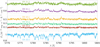 |
Fig. 8 Flux-subtraction of the ES 22.5 spectrum from the other ESPRESSO spectra. The top panel shows the five subtracted spectra median filtered to three points. ES 22.5 is shown in the bottom panel for reference. |
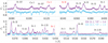 |
Fig. 9 Comparison between the ES 21.1 and ES 22.5 spectra in regions dominated by metallic emission lines. Species producing line emission are marked. The Fe I 5447, Si II 6347, and Ca I 6122 lines used in Sec. 6.1 are marked in red. |
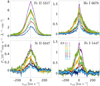 |
Fig. 10 Continuum subtracted profiles of the Fe II 5317, He I 6678, Si II 6347, and Fe I 5447 lines in the ESPRESSO spectra. |
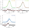 |
Fig. 11 Subtraction between consecutive Fe II 5317 ESPRESSO spectra. The color code is the same as in Fig. 10. The profiles were rescaled by a constant (upper right corner). The bottom panels show the subtracted profiles, with Gaussian fits superposed. |
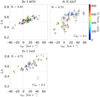 |
Fig. 12 Relation between vBC and LA for the He I 6678, Si II 6347, and Fe I 5447 lines. R is the Pearson correlation coefficient. |
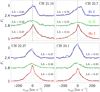 |
Fig. 13 Selected observations showing the variability of the asymmetry of the He I 6678, Si II 6347, and Fe I 5447 lines. Here, LA is the line asymmetry to the blue. |
6 TESS light curve
The TESS Sector 65 light curve of RU Lup is displayed in Fig. 14. We converted the TESS pre-search data conditioning simple aperture photometry (PDCSAP) flux (F) into TESS magnitudes T using the relation T = −2.5 log10 F + ZP, where ZP = 20.44 is the TESS Zero Point magnitude (Vanderspek et al. 2018). The time t is computed relative to the MJD of the beginning of the observation (MJDbeg = 60068.25).
If the hot spot has a photometric signature, we expect its maximum contribution at phase ϕS (Sec. 4), marked with dashed blue lines in Fig. 14. This phase is a quarter of period after the maximum blueshift and a quarter of period before the maximum redshift of the hot spot, hence it is the position where the spot area projected along the line of sight is maximum. For most cycles this phase does not coincide with a maximum in the TESS light curve. This suggests that either the hot spot does not contribute significantly to the photometry or the period detected from the analysis of the NC is not the actual rotation period of the spot. We further discuss this issue in Sec. 7.
The light curve displays two epochs of quasi-periodic bursts superposed on a base level of ~10.2 mag. In the first epoch the system reaches 9.5 mag as maximum brightness. In the second epoch this value is reduced to 9.8 mag. The transition between these two regimes is at t ≈ 9.15 days. A visual inspection of the light curve suggests that the typical timescale of the variability is smaller than P*. This can be seen, for example, between ϕ = 1.7 and ϕ = 2.7, where we observe three maxima instead of one.
We used the continuous wavelet analysis to determine the frequency content of the light curve as a function of time. In the analysis of the QPOs, we used the quality factor as a measure of the coherence of the oscillations. It is defined as Q = P0/ΔP, where P0 is the detected period and ΔP is the FWHM of the peak. The continuous wavelet transform (CWT) of the light curve (Fig. 15) reveals how these two segments have a different frequency content. To refine the estimate of the timescales, we computed a separate Lomb-Scargle Periodogram (LSP) for each segment of the light curve. For both segments, we detected a double-peaked structure in the LSP. There is power around P* but the peak is broad, that is, the oscillations are not coherent. For t ≲ 9.15 days, we obtained P = 1.31 ± 0.06 days with Q ≈ 9.1 and P = 2.15 ± 0.14 days with Q ≈ 6.5. For t ≳ 9.15 days, we found instead P = 1.66 ± 0.07 days with Q ≈ 10.1 and P = 2.08 ± 0.10 days with Q ≈ 8.7. The 1σ uncertainties were obtained from the quality factor by converting the FWHM to the standard deviation of a Gaussian ![Mathematical equation: $\[(\mathrm{FWHM}=2 \sqrt{2 \ln 2} \sigma)\]$](/articles/aa/full_html/2024/10/aa51065-24/aa51065-24-eq9.png) . A similar multiple-peak structure of the LSP is observed in 3D MHD simulations (e.g., Kulkarni & Romanova 2009) and indicates that the oscillations are not purely sinusoidal (Romanova & Kulkarni 2009).
. A similar multiple-peak structure of the LSP is observed in 3D MHD simulations (e.g., Kulkarni & Romanova 2009) and indicates that the oscillations are not purely sinusoidal (Romanova & Kulkarni 2009).
For both time segments, the shorter period has the higher quality factor, and we propose that this period is the actual timescale of the oscillations. We show this by superposing a sinusoidal oscillation with that period on the relative portion of the light curve. The sine function is parameterized as mag(t) = C + A sin[2π(t − t0)/P]. We adjusted the free parameters of the sine function (i.e., C, A, and t0) in order to visually reproduce the behavior of the QPOs. To do this, we further split the second segment in two parts, with separation at t ≈ 15.75 days. This is the time where the light curve returns to the base level, after which the oscillations seem to be delayed by ~0.5 days. Figure 15 shows the results of this procedure. Most of the maxima in the sinusoids match a peak in the TESS light curve. The cycle-to-cycle variability indicates that the environment traced by TESS changes on dynamical (1–2 days) timescales. We conclude that P1 = 1.31 days and P2 = 1.66 days are the typical timescales of the variability, while the higher period peaks in the LSPs are due to the non-sinusoidal nature of the oscillations. In the RT-unstable accretion scenario, these periods are interpreted as the Keplerian periods at the truncation radius RT.
6.1 Contemporaneous CHIRON spectroscopy
The maximum magnitude level reached in the two segments of the TESS Sector 65 light curve differs by ~0.3 mag, that is, a factor ~30% in flux. The system attains the higher flux in the first segment, where the detected period is lower. 3D MHD simulations of accretion through a MBL showed how an increase in ![Mathematical equation: $\[\dot{M}_{\mathrm{acc}}\]$](/articles/aa/full_html/2024/10/aa51065-24/aa51065-24-eq10.png) leads to a decrease in the detected period (Romanova & Kulkarni 2009). If the flux increase is caused by an increase in
leads to a decrease in the detected period (Romanova & Kulkarni 2009). If the flux increase is caused by an increase in ![Mathematical equation: $\[\dot{M}_{\mathrm{acc}}\]$](/articles/aa/full_html/2024/10/aa51065-24/aa51065-24-eq11.png) , the change of the QPO period within the TESS Sector 65 light curve is an observational signature of RT moving toward the star. The spectroscopic data from CHIRON confirm this hypothesis. Table A.1 shows that among the CHIRON observations from 2023 the first three spectra, which are taken in the epoch of highest flux, have the highest veiling. Figure 16 shows the Fe I 5447, Si II 6347, and Ca I 6122 lines in the 9 CHIRON observations that are simultaneous to the TESS Sector 65 light curve. The first three spectra are the ones with the higher EW of these lines, indicating that the system is in a state of higher accretion rate in the first portion of the light curve (see the discussion in Sec. 5). Assuming a constant B* during the TESS observing run, the ratio P1/P2 can be converted to a ratio between accretion rates. Since
, the change of the QPO period within the TESS Sector 65 light curve is an observational signature of RT moving toward the star. The spectroscopic data from CHIRON confirm this hypothesis. Table A.1 shows that among the CHIRON observations from 2023 the first three spectra, which are taken in the epoch of highest flux, have the highest veiling. Figure 16 shows the Fe I 5447, Si II 6347, and Ca I 6122 lines in the 9 CHIRON observations that are simultaneous to the TESS Sector 65 light curve. The first three spectra are the ones with the higher EW of these lines, indicating that the system is in a state of higher accretion rate in the first portion of the light curve (see the discussion in Sec. 5). Assuming a constant B* during the TESS observing run, the ratio P1/P2 can be converted to a ratio between accretion rates. Since ![Mathematical equation: $\[P_{\mathrm{T}} \propto R_{\mathrm{T}}^{3 / 2}\]$](/articles/aa/full_html/2024/10/aa51065-24/aa51065-24-eq12.png) and
and ![Mathematical equation: $\[R_{\mathrm{T}} \propto\left(B_{\star}^2 / \dot{M}_{\mathrm{acc}}\right)^{2 / 10}\]$](/articles/aa/full_html/2024/10/aa51065-24/aa51065-24-eq13.png) (Eq. (1)), we find
(Eq. (1)), we find ![Mathematical equation: $\[\dot{M}_{\mathrm{acc}, 1} / \dot{M}_{\mathrm{acc}, 2}=\left(P_1 / P_2\right)^{-10 / 3} \approx 2.2\]$](/articles/aa/full_html/2024/10/aa51065-24/aa51065-24-eq14.png) .
.
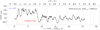 |
Fig. 14 TESS light curve of RU Lup from Sector 65 (2023). The light curve is plotted as a function of the time t from the beginning of the observation (MJDbeg = 60068.25). The top axis show the phase ϕ computed with P = 3.63 days (i.e., the spot period, Sec. 4.1). The reference date for ϕ = 0 is MJD0 ≡ 59264.336. The blue lines mark the phase ϕS (from Sec. 4.1), where the maximum contribution from the hot spot is expected. The red lines mark the epochs of the CHIRON spectroscopic observations. |
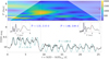 |
Fig. 15 Continuous wavelet analysis of the TESS Sector 65 light curve. The top panel shows the CWT. The bottom panel displays the light curve. The insets show the LSP for the two portions of the light curve. The blue and red lines mark the detected period and P*, respectively. Sinusoidal oscillations are superposed to the TESS observation in green, with the period of the oscillations in each portion reported with the same color. |
6.2 Oscillations from a nonstationary hot spot
All timescales observed in the TESS light curve are shorter than the stellar rotation period. There are two regions that can produce variability at such timescales: a non-axisymmetric portion of the disk that extends inward of Rco and rotates around the star (Sicilia-Aguilar et al. 2023), or a nonstationary hot spot on the surface of the star (Romanova & Kulkarni 2009).
A simple, planar portion of the disk which revolves around the star such as the one proposed by Sicilia-Aguilar et al. (2023) cannot account for the quasi-periodic variability observed in RU Lup. The reason is that the angle between the surface of the disk and the line of sight is constant, since the disk lies on a plane. If the structure is located in the disk, it must have a more complicated configuration, such that its projected surface changes as it revolves around the star.
On the other hand, a moving hot spot on the surface of the star can reproduce the observed variability, since its projected area varies with the azimuthal position as the spot rotates. The amplitude and zero point of the oscillations observed with TESS can be reproduced with an analytical model, assuming a spot with temperature T and filling factor f, located at a latitude θS on the stellar surface (Appendix D). We analyzed the two portions of the light curve with different maximum fluxes separately. We obtained θS1 = 61° and θS2 = 65° for the latitude of the spot in the two segments (Eq. (D.7)). Figure 17 shows the degenerate relation between the filling factor and the temperature of the spot that best fits the modulations in the light curve (Eq. (D.8)). The analytical model indicates that the spot is either more extended or hotter, or both, during the epoch of increased accretion (t ≤ 9.15 days in Fig. 17).
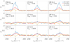 |
Fig. 16 Normalized profiles of the Fe I 5447, Si II 6347, and Ca I 6122 lines in the 9 CHIRON spectra that are contemporaneous to the TESS Sector 65 light curve. Tmag is the TESS magnitude at these epochs. |
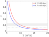 |
Fig. 17 Relation between the filling factor (f) and the temperature (T) (Appendix D), for a spot that reproduces the modulations observed in the TESS Sector 65 light curve. The gray area marks 0.18 ≤ f ≤ 0.26 (Wendeborn et al. 2024a), while the dashed line marks f = 0.12 (Dodin & Lamzin 2012). |
7 Discussion
There are two main results of this work. First, the narrow component of the He I 5876 line is modulated with a period of 3.63 days, close to P* = 3.71 days derived by Stempels et al. (2007) from the radial velocity changes in the absorption lines of RU Lup. The fact that vNC is in anti-phase with vphot indicates that the photospheric lines are distorted by narrow emission components produced in a hot spot (Sec. 4.3) and not by a cold spot as suggested by Stempels et al. (2007).
Second, the timescales detected in the TESS light curve of RU Lup are shorter than P*, and they can be interpreted as evidence of accretion from inward of Rco. The photometric variability can be produced by either a complex warped structure in the disk or spot(s) on the stellar surface. In addition, we observed a change in the period throughout the TESS light curve that appears to be related to variations in ![Mathematical equation: $\[\dot{M}_{\mathrm{acc}}\]$](/articles/aa/full_html/2024/10/aa51065-24/aa51065-24-eq15.png) . In the rest of the section, we discuss scenarios that might explain the discrepancy between the timescales detected in spectroscopy and photometry. We conclude the discussion with the analysis of the accretion flow inferred from the emission lines.
. In the rest of the section, we discuss scenarios that might explain the discrepancy between the timescales detected in spectroscopy and photometry. We conclude the discussion with the analysis of the accretion flow inferred from the emission lines.
7.1 TESS light curve and regime of accretion
The study of the frequency spectrum of the TESS light curve allows us to obtain an indirect measure of the position of the truncation radius RT. Interpreting P1 = 1.31 days and P2 = 1.66 days (Sec. 6) as the Keplerian rotation at the truncation radius RT, we convert these measures to positions of RT using RT/Rco = (PT/P*)2/3. We obtain RT = 0.5 Rco for the first epoch and RT = 0.59 Rco for the second epoch. The derived RT/Rco ratios indicate that RU Lup accretes in a RT-unstable regime (Blinova et al. 2016; Pantolmos et al. 2020), in agreement with the result by Stock et al. (2022). Together with the estimate of Rco (Table 1), we find that RT is approximately 2 R* (~1.82 R* and ~2.15 R* for the first and second epoch, respectively).
The position of the truncation radius can be estimated independently, knowing ![Mathematical equation: $\[\dot{M}_{\mathrm{acc}}\]$](/articles/aa/full_html/2024/10/aa51065-24/aa51065-24-eq16.png) and B* (Eq. (1)). We obtained an estimate of
and B* (Eq. (1)). We obtained an estimate of ![Mathematical equation: $\[\dot{M}_{\mathrm{acc}}\]$](/articles/aa/full_html/2024/10/aa51065-24/aa51065-24-eq17.png) for the CH 23.4 spectrum4 using the He I 5876 line as follows. We calculated the line luminosity from the integrated flux of the line using the Gaia DR3 distance (Table 1) and converted it to an accretion luminosity (Lacc) using the relation calibrated by Alcalá et al. (2017). Then, assuming that the free-fall starts at Rco (i.e., RT = Rco), we derived
for the CH 23.4 spectrum4 using the He I 5876 line as follows. We calculated the line luminosity from the integrated flux of the line using the Gaia DR3 distance (Table 1) and converted it to an accretion luminosity (Lacc) using the relation calibrated by Alcalá et al. (2017). Then, assuming that the free-fall starts at Rco (i.e., RT = Rco), we derived ![Mathematical equation: $\[\dot{M}_{\mathrm{acc}}\]$](/articles/aa/full_html/2024/10/aa51065-24/aa51065-24-eq18.png) by inverting the relation
by inverting the relation
![Mathematical equation: $\[L_{\mathrm{acc}}=\frac{G M_{\star} \dot{M}_{\mathrm{acc}}}{R_{\star}}\left(1-\frac{R_{\star}}{R_{\mathrm{T}}}\right)\]$](/articles/aa/full_html/2024/10/aa51065-24/aa51065-24-eq19.png) (3)
(3)
(Hartmann et al. 2016). We obtained ![Mathematical equation: $\[\dot{M}_{\mathrm{acc}}\]$](/articles/aa/full_html/2024/10/aa51065-24/aa51065-24-eq20.png) = 1.48 × 10⁻⁷ M⊙ yr−1. Using the upper limit of ~0.5 kG derived by Johnstone & Penston (1986) for the dipolar magnetic field of RU Lup, we find an upper limit of 2.1 R* for RT, in good agreement with the values inferred photometrically5.
= 1.48 × 10⁻⁷ M⊙ yr−1. Using the upper limit of ~0.5 kG derived by Johnstone & Penston (1986) for the dipolar magnetic field of RU Lup, we find an upper limit of 2.1 R* for RT, in good agreement with the values inferred photometrically5.
Blinova et al. (2016) showed that the unstable regime can be divided in two sub-regimes; namely, the chaotic regime and the ordered (or MBL, Romanova & Kulkarni 2009) regime. The difference between the two regimes is in the stability of the QPOs. In the chaotic regime, short-lived hot spots, which last for only a few rotations around the star, produce short-duration QPOs (Kulkarni & Romanova 2009). In the MBL regime, the QPOs are more stable (Romanova & Kulkarni 2009). The clear QPOs observed throughout the TESS Sector 65 light curve are more compatible with the latter regime of accretion. The values of RT/Rco that we derived above are in agreement with the results of 3D MHD simulations of accretion in the MBL regime (RT/Rco ≲ 0.59, Blinova et al. 2016). In this scenario, accretion proceeds in two ordered tongues controlled by the RT instability, which produce hot spots on the surface of the star.
7.2 Properties of the hot spot inferred from spectroscopy
The radial velocity amplitude of the He I 5876 NC modulation is smaller than v sin i, indicating that the NC-emitting region is located on the stellar surface, at high latitude. The NC emission in high energy lines (e.g., He I and He II) identify this region as the post-shock region.
The red asymmetry observed in the NC of the He I line, with emission up to ~+100 km s−1 (i.e., ~3σr for He I, Fig. 6) is compatible with formation in the post-shock region, where the gas decelerates to 1/4 of the pre-shock velocity (Hartmann et al. 2016). The blue wing of the line might be indicative of the broadening mechanism, with either thermal or turbulent motions that broaden the emission line. Using σ = (2kBT/Amp)1/2, where kB is the Boltzmann constant, mp is the proton mass, and A = 4 is the atomic number of helium, we get an upper limit of ~50000 K for the temperature of the post-shock region from σb, = 14 km s−1 (Fig. 6). The post-shock region cools in X-rays (Lamzin 1999; Sacco et al. 2008) and high energy ultraviolet lines (Ardila et al. 2013). Therefore, we do not expect it to directly contribute in the TESS bandpass. In that wavelength range, most of the contribution comes from the heated photosphere below the shock (Calvet & Gullbring 1998). This region is heated from above by 3/4 of the shock energy, reaching temperatures up to ~8000 K (Hartmann et al. 2016).
Dodin & Lamzin (2012) showed that the heated photosphere not only emits in the continuum, but is also responsible for the emission in the NC of the metallic species. The NCs are formed in a layer with a temperature inversion (i.e., a chromospheric-like structure) above the continuum-emitting region. Our analysis of the NCs possibly highlights the vertical stratification of this layer. The more energetic lines (Fe II and Si II) are indeed more asymmetric to the red than the less energetic ones (Fe I and Mg I), suggesting that the former could originate in the upper part of this structure (at higher T) and still have a residual infall velocity, as sketched in Fig. 18.
In Sect. 4.4, we showed how the veiling spectrum of RU Lup at 5800 Å is composed of a continuum plus line emission that fills in the photospheric absorption lines. The anticorrelation between vNC of the He I 5876 line and vphot (Sec. 4.3) imply that the veiling spectrum is formed in a confined region on the stellar surface, in other words, a spot. This spot, which we identify as the heated photosphere below the post-shock region, must also contribute to the emission in the TESS bandpass, which extends from 5800 to 11 200 Å.
7.3 Properties of the hot spot inferred from photometry
By using the analytical model of Appendix D, we were able to infer the properties of the photometric spot, assuming that it is nonstationary on the surface of the star. The degeneracy between the filling factor and the temperature of the spot can be removed by considering values of f from the literature. Using a typical value of f ≈ 0.05 for CTTSs (Calvet & Gullbring 1998; Calvet et al. 2004), we get a temperature of ~20000 K for the spot. However, specific works on RU Lup showed how the filling factor of the spot is higher than the usual values for CTTSs. In Fig. 17 we report the values obtained by Wendeborn et al. (2024a) from a best fit of the 2021 ultraviolet spectra of RU Lup with a shock model (0.18 ≤ f ≤ 0.26) and the value derived by Dodin & Lamzin (2012) by fitting the veiling spectrum of RU Lup (f = 0.12). In these cases, we obtain a colder spot with T ~ 8000 − 12000 K, more compatible with the typical values for CTTSs (Hartmann et al. 2016).
Assuming a spherical cap geometry for the spot (Appendix E), and a filling factor between 0.1 and 0.2 as mentioned in the previous literature of RU Lup, the half-opening angle of the spot is between 37° and 57°. If the hot spot is as extended as that, then the spot model from Appendix D is too simplistic and the derived θS must be regarded as an average latitude of the continuum-emitting region.
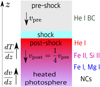 |
Fig. 18 Sketch of the possible vertical stratification of the hot spot inferred from the analysis of the NCs. vpre and vpost are the pre-shock and post-shock velocities. |
7.4 Comparison between spectroscopy, photometry, and magnetohydrodynamic simulations of the spot
The spectroscopic results on the hot spot seem to disagree with what is derived from the analysis of the TESS light curve and with the results of 3D MHD simulations of a system accreting in the MBL regime, due to the latitude/extension of the spots and the detected timescales. We propose that the spectroscopic and photometric spot are part of the same structure, which we identify as the region in which the accreting gas impacts the stellar surface. The He I NC – that is, the tracer of the spectroscopic spot – originates in the post-shock region. The continuum emission in the TESS bandpass, associated with the photometric spot, is formed instead in the heated photosphere below the shock. This region emits also in the NC of the metallic species and it is responsible for the line-filling component of the veiling (Dodin & Lamzin 2012).
Considering the typical extension of the spot in RU Lup (f ≈ 0.1–0.2), we might expect a discrepancy between the latitude derived from spectroscopy and photometry. The region traced by the He I NC (i.e., the post-shock region) must be somewhat less extended than the heated photosphere traced by TESS. Otherwise, considering the low inclination of the system and the intrinsic variability of this region as a consequence of the accretion process, it would be impossible to detect a rotational modulation (Sicilia-Aguilar et al. 2023).
A possible explanation of the inconsistency in the detected periods lies in the variability of the mass accretion rate. The 3.63 day period was derived in Sec. 4.1 using data from epochs that have different ![Mathematical equation: $\[\dot{M}_{\mathrm{acc}}\]$](/articles/aa/full_html/2024/10/aa51065-24/aa51065-24-eq21.png) . In Sec. 6 we discussed how variations in the accretion rate lead to variations in the detected period. Stock et al. (2022) showed that the accretion rate of RU Lup varies by a factor of ~2 on a timescale of weeks. Since
. In Sec. 6 we discussed how variations in the accretion rate lead to variations in the detected period. Stock et al. (2022) showed that the accretion rate of RU Lup varies by a factor of ~2 on a timescale of weeks. Since ![Mathematical equation: $\[P_{\mathrm{T}} \propto \dot{M}_{\mathrm{acc}}^{-3 / 10}\]$](/articles/aa/full_html/2024/10/aa51065-24/aa51065-24-eq22.png) (Eq. (1)), this means that the period of a nonstationary hot spot would vary by a factor of 23/10 ≈ 1.23 on such timescales. If the He I 5876 NC traces a nonstationary hot spot on the stellar surface produced by tongues originating at RT, it is plausible that its radial velocity is modulated with both P* and the inner disk period (PT). In this situation, if one were to look for periodicity combining observations that represent different accretion states, the power at P* would be enhanced in the periodogram because of the stability of this period among different epochs.
(Eq. (1)), this means that the period of a nonstationary hot spot would vary by a factor of 23/10 ≈ 1.23 on such timescales. If the He I 5876 NC traces a nonstationary hot spot on the stellar surface produced by tongues originating at RT, it is plausible that its radial velocity is modulated with both P* and the inner disk period (PT). In this situation, if one were to look for periodicity combining observations that represent different accretion states, the power at P* would be enhanced in the periodogram because of the stability of this period among different epochs.
These complications are illustrated in Fig. 19, where we recomputed the LSP of the He I 5876 NC using only the data from 2022. The periodogram has maximum power at P = 1.38 days, but the FAP of this signal is >30%; that is, it is not statistically significant. The second highest peak is close to P*. The period with maximum power is similar to the periods derived from TESS. This suggests that the apparent lack of continuum emission from the spot (Sec. 6) could be actually caused by an incorrect phase-folding of the radial velocity of the He I 5876 NC. If the period of the hot spot is not correct, then the phase ϕS where we expect its maximum contribution is different from what we derived, and might be in agreement with maxima in the TESS light curve.
Therefore, we conclude that in the MBL picture the disagreement between the period detected from spectroscopy (P*) and the period inferred from photometry (<P*) might be attributed to an observational problem, namely, the difficulty of tracing a hot spot that rotates with the inner disk period, with the latter being sensitive to variations in ![Mathematical equation: $\[\dot{M}_{\mathrm{acc}}\]$](/articles/aa/full_html/2024/10/aa51065-24/aa51065-24-eq23.png) .
.
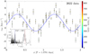 |
Fig. 19 Radial velocity curve of the He I 5876 NC for the 2022 observations only. The inset shows the LSP, with the detected P and P* marked with dashed blue and red lines, respectively. |
7.5 Alternative explanations: sub-structure of the spot and inner disk warp
Although accretion in the MBL regime can explain the photometric behavior of RU Lup, the detected periods are close to P*/2. Hence, the photometric behavior could also be explained with a modulation at a period close to P* but with a brightness distribution on the visible hemisphere more closely resembling two hot spots; that is, a single, extended hot spot that has a non-homogeneous surface brightness, such that we see two brighter features. The brightness distribution of this region could vary on dynamical timescales and the detected periods could be aliases produced by the complex structure of this region. Similarly, the change in the quasi-period between the two epochs of the TESS light curve could be due to an intrinsic variability in the shape and brightness of this extended spot. Since the velocity modulation of emission lines mainly traces the average brightness distribution, a large non-homogeneous spot would lead to a modulation at ~P* in the radial velocity of the NCs, as we observe for the He I 5876 line.
Periods close to P* would be compatible with a scenario in which RU Lup is in a stable accretion regime. However, 3D MHD simulations of accretion in the stable regime showed how the spots are formed close to the magnetic pole and are antipodal (e.g., Romanova et al. 2003, 2004) so that it is unlikely to see two distinct, antipodal spots given the low inclination (i* = 16 ± 6 °) of the stellar rotation axis in RU Lup. Rather, the brightness modulation would require sub-structure of a single spot. MHD simulations of accretion in the stable regime predict the hot spots to be bow-shaped around the magnetic axis (Romanova et al. 2004) with a temperature gradient from the center to the edges (Kulkarni & Romanova 2013); that is, a structure that is different from the requirements of period aliasing. Hence, the structure of the hot spot must be somewhat different from what is predicted by 3D MHD simulations if accretion in RU Lup proceeds in the stable regime. Moreover, independent of the true variability, the TESS light curve shows that the dominant periodicity changes, with the shorter period pertaining to epochs with higher (optical) luminosity, in agreement with MHD models of accretion in the unstable regime (Kulkarni & Romanova 2009). Therefore, we think that the MBL scenario fits the observations better than the hypothesis of accretion in a stable regime.
A third explanation is motivated by the high values of the filling factor that we derived for RU Lup. Such a high (0.1–0.2) filling factor could be achieved if the part of the continuum-emitting region lies in the disk. In Sec. 6.2 we discussed how a structure located in the disk must have a complex geometry in order to produce a quasi-periodic modulation. A warp in the inner disk inward of Rco might satisfy this condition, and would naturally explain the observed timescales. In this scenario, the continuum emitting region would be spatially separated from the region emitting in the NCs, because the latter is unequivocally associated with shocked gas on the stellar surface. Such a structure could be characteristic of systems accreting through a compact magnetosphere, and it might be a non-axisymmetric version of the classical boundary layer. To our knowledge, no models of quasi periodic oscillations from a warped structure in the disk have been studied.
7.6 Inner disk dynamics
7.6.1 Structure of the flow
The width of the metallic lines points toward an origin in the circumstellar matter. Their velocity centroids (vBC) are between −30 and +60 km s−1 (Fig. 12), compatible with the projected velocities of flows within the inner disk. For a Keplerian disk seen at an inclination i, the radial velocity is
![Mathematical equation: $\[v_{\mathrm{rad}}\left(r, \phi_{\mathrm{D}}\right)=\sqrt{\frac{G M_{\star}}{r}} \sin i \sin \phi_{\mathrm{D}}\]$](/articles/aa/full_html/2024/10/aa51065-24/aa51065-24-eq24.png) (4)
(4)
where r is the distance from the star and ϕD is the azimuth relative to the observer (e.g., Horne & Marsh 1986). For i = 16° (Table 1), we get a maximum vrad of ~50, 45, 40, and 30 km s−1 for r = 0.4, 0.5, 0.6, and 1 Rco. Hence, the observed vBC values are compatible with the position of the truncation radius derived from TESS data, suggesting that the lines are formed in a disk-like structure that revolves around the star.
To reproduce the variability of the line asymmetry, this structure must be non-axisymmetric, and it might look like a portion of a Keplerian disk, as proposed by Sicilia-Aguilar et al. (2023) to model the BC variability of the Ca II lines in EX Lup. However, the lines are much broader than the maximum vrad that can be observed from a Keplerian disk, that is, (GM*/R*)1/2 sin i ≈ 60 km s−1 for RU Lup. Therefore, they are either broadened by turbulent motions in the Keplerian portion of the disk, as proposed by Sicilia-Aguilar et al. (2023), or formed in a flow with higher velocities.
In the case of RU Lup, the analysis of the Fe II 5317 line (Fig. 11) reveals how a turbulent portion of a Keplerian disk cannot completely account for the line velocities. The discrete emission components detected with the subtraction of consecutive spectra have centroids – bulk velocities >(GM*/R*)1/2 sin i – indicating that part of the line emission is produced by macroscopic flows in non-Keplerian motion.
Radial velocities of the order of 100–150 km s−1 are compatible with free fall along dipolar magnetic field lines. The free fall velocity starting from rest at RT is
![Mathematical equation: $\[v_{\mathrm{ff}}(r)=\sqrt{G M_{\star}\left(\frac{1}{r}-\frac{1}{R_{\mathrm{T}}}\right)}.\]$](/articles/aa/full_html/2024/10/aa51065-24/aa51065-24-eq25.png) (5)
(5)
For RT = 2 R* (Sec. 6) we get vff(R*) ≈ 205 km s−1. The observed velocity is significantly lower for a pole-on system, because the velocity vector of the gas moving along the magnetic field lines is almost transverse to the line of sight. The observed radial velocity is reduced by a factor
![Mathematical equation: $\[\frac{(3 / 2) \sin 2 \theta \cos \phi \sin i+\left(2-3 \cos ^2 \theta\right) \cos i}{\sqrt{4-3 \cos ^2 \theta}}\]$](/articles/aa/full_html/2024/10/aa51065-24/aa51065-24-eq26.png) (6)
(6)
(Calvet & Hartmann 1992; Wilson et al. 2022). Here, θ is the latitude, ϕ is the azimuth relative to the observer, and the gas is assumed to be moving along a dipolar streamline with equation r = RT cos2 θ. The maximum redshifted and blueshifted radial velocities that can be observed are obtained for ϕ = 0 and π and are +110 and −60 km s−1, respectively, assuming RT = 2 R*. The fact that the maximum negative vrad is lower than maximum positive vrad is a projection effect. This red-blue asymmetry is similar to the variation in vBC for RU Lup throughout our observations. This argues in favor of line formation in a magnetospheric accretion column and against formation in a structure that is confined to a plane, such as a Keplerian disk or equatorial accretion tongues. In that case, the redshifted and blueshifted line shifts would be the same.
7.6.2 Temperature stratification
The different line widths, which correlate with the excitation energy of the analyzed emission lines (Sec. 5), indicate the existence of a stratification in the accretion flow of RU Lup. The He I lines must be formed close to the shock in high temperature conditions, and their higher FWHM relative to the Fe I and Si II lines indicate a formation in a flow with higher velocities. Conversely, neutral species like Fe I and Ca I are formed closer to the disk, where the material starts to accrete onto the star in accretion tongues. This region must be non-axisymmetric in order to explain the line variability, and it might be similar to the azimuthally-limited Keplerian disk proposed by Sicilia-Aguilar et al. (2023). The singly ionized species such as Fe II and Si II have velocities that are not consistent with Keplerian flows, and require higher temperature conditions than what can be achieved in an irradiated disk. The extreme line asymmetry to the red that is sometimes observed in the Si II 6347 line (see Fig. 13) suggests that these species are partly formed in the flow along the magnetic field lines. The different line asymmetry observed for emission lines from the same observation support the stratification hypothesis, since lines tracing different regions of the accretion flow might be asymmetric at different times.
In conclusion, the variability of the He I and metallic lines can be explained with the lines being formed in a temperature stratified structure which is a combination of a non-axisymmetric Keplerian disk and an inflow along magnetic field lines. This structure is sensitive to variations in the accretion rate.
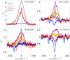 |
Fig. 20 A selection of metallic lines in the spectra of RU Lup, HM Lup, and Sz 98. |
7.7 Formation of the metallic lines
Analogous to the case of the H I, He I, and Ca II lines (Alcalá et al. 2017), one would expect the strength of the metallic lines to be dependent on ![Mathematical equation: $\[\dot{M}_{\mathrm{acc}}\]$](/articles/aa/full_html/2024/10/aa51065-24/aa51065-24-eq27.png) . Figure 20 compares RU Lup with two other CTTSs; namely HM Lup, which shows prominent metallic emission, and Sz 98, which has the same stellar parameters of RU Lup (Manara et al. 2023). We show the second ESPRESSO observation analyzed by Armeni et al. (2023) for HM Lup, and an Ultraviolet and Visual Echelle Spectrograph (UVES, Dekker et al. 2000) spectrum taken on 10/05/2022 as part of the PENELLOPE survey for Sz 98. The accretion rates for HM Lup and Sz 98, taken from the literature, are 0.95 × 10⁻⁸ M⊙ yr−1 (Armeni et al. 2023) and 3.6 × 10⁻⁸ M⊙ yr−1 (Manara et al. 2023), respectively.
. Figure 20 compares RU Lup with two other CTTSs; namely HM Lup, which shows prominent metallic emission, and Sz 98, which has the same stellar parameters of RU Lup (Manara et al. 2023). We show the second ESPRESSO observation analyzed by Armeni et al. (2023) for HM Lup, and an Ultraviolet and Visual Echelle Spectrograph (UVES, Dekker et al. 2000) spectrum taken on 10/05/2022 as part of the PENELLOPE survey for Sz 98. The accretion rates for HM Lup and Sz 98, taken from the literature, are 0.95 × 10⁻⁸ M⊙ yr−1 (Armeni et al. 2023) and 3.6 × 10⁻⁸ M⊙ yr−1 (Manara et al. 2023), respectively.
The comparison between the spectrum of HM Lup and the ES 22.5 spectrum of RU Lup shows that despite ![Mathematical equation: $\[\dot{M}_{\mathrm{acc}}\]$](/articles/aa/full_html/2024/10/aa51065-24/aa51065-24-eq28.png) being one order of magnitude lower for HM Lup, the emission line profiles are very similar. The only strong emission line is Fe II 5317. The Fe I 5447 and Si II 6347 lines are weak, while the Ca I 6122 is in absorption in both spectra. Although Sz 98 has
being one order of magnitude lower for HM Lup, the emission line profiles are very similar. The only strong emission line is Fe II 5317. The Fe I 5447 and Si II 6347 lines are weak, while the Ca I 6122 is in absorption in both spectra. Although Sz 98 has ![Mathematical equation: $\[\dot{M}_{\mathrm{acc}}\]$](/articles/aa/full_html/2024/10/aa51065-24/aa51065-24-eq29.png) between HM Lup and RU Lup, Fig. 20 shows how the metallic lines are very weak in its spectrum. The only detectable emission is in Fe II 5317, with the line being slightly above the continuum. This suggests that the strength of these transitions relative to the continuum is not directly related to
between HM Lup and RU Lup, Fig. 20 shows how the metallic lines are very weak in its spectrum. The only detectable emission is in Fe II 5317, with the line being slightly above the continuum. This suggests that the strength of these transitions relative to the continuum is not directly related to ![Mathematical equation: $\[\dot{M}_{\mathrm{acc}}\]$](/articles/aa/full_html/2024/10/aa51065-24/aa51065-24-eq30.png) . We propose that the actual parameter that controls the strength of the metallic lines is the ratio RT/Rco. The smaller this ratio is, the stronger the emission lines are. Different species appear at different RT/Rco ratios, with the Fe II lines being the first ones that show up, followed by the Fe I and Si II lines, and, finally, from the Ca I λλ 6103, 6122 doublet. This transition is visually illustrated by the ES 22.5, ES 22.2 and ES 21.1 spectra in Fig 20.
. We propose that the actual parameter that controls the strength of the metallic lines is the ratio RT/Rco. The smaller this ratio is, the stronger the emission lines are. Different species appear at different RT/Rco ratios, with the Fe II lines being the first ones that show up, followed by the Fe I and Si II lines, and, finally, from the Ca I λλ 6103, 6122 doublet. This transition is visually illustrated by the ES 22.5, ES 22.2 and ES 21.1 spectra in Fig 20.
If related to RT/Rco, emission in metallic species is a direct indication of accretion in the RT-unstable regime. This can be explained by a simple energetic argument. When RT < Rco, the material at RT rotates faster than the star. Since the magnetic field lines co-rotate with the star, the gas must dissipate energy and angular momentum in order to accrete. This dissipation could give rise to the local heating required to collisionally excite the metallic lines (Beristain et al. 1998).
8 Conclusions
We have presented a spectrophotometric study of the CTTS RU Lup. Figure 21 shows a schematic picture of the circumstellar environment of RU Lup that we inferred from our observations. The main results are the following.
We have improved the measurement of the stellar parameters, summarized in Table 1.
We detected a modulation at a period of 3.63 days, close to P* = 3.71 days (Stempels et al. 2007), in the NC of the He I 5876 line, indicating the presence of a compact region on the stellar surface that we identify as the post-shock region that originates at the footprint of the magnetic field.
The heated photosphere below the accretion shock (i.e., a hot spot) is also responsible for the veiling of the photospheric lines in the spectrum.
This veiling spectrum is composed of a continuum component plus line emission that fills in the stellar absorption lines. The use of flux-calibrated, high-resolution spectra allowed us to disentangle these two contributions.
We detected timescales shorter than P* in the TESS light curve of RU Lup. These timescales are related to the Keplerian period at the truncation radius, RT.
From these timescales, we inferred the size of the magnetosphere of RU Lup to be −2 R*.
The behavior of the TESS Sector 65 light curve of RU Lup is consistent with simulations of accretion through a MBL (Romanova & Kulkarni 2009), in which the QPOs are produced by a non-stationary hot spot on the stellar surface.
The hot spot is not as equatorial as predicted by the MHD simulations of accretion in the MBL regime, and it appears to be more extended than in typical CTTSs, with a filling factor of ~0.1–0.2.
Alternatively, more complex explanations would require either a spot with a complex shape, perhaps made of two brighter knots which vary on dynamical timescales, or a warped structure in the inner disk.
The BCs are formed in a non-axisymmetric, temperature stratified flow around the star in which the gas leaves the accretion disk at RT and accretes onto the star in tongues of matter channeled by the magnetic field.
The strength of the metallic emission lines might be an indicator of accretion in the RT-unstable regime, being related to the ratio between RT and Rco.
The spectrophotometric analysis presented in this work revealed the complexity of the accretion process in RU Lup, and showed how the physics regulating the accretion flow in this system might be somewhat different from the current theoretical paradigms of accreting CTTSs. Future studies should aim at covering high-cadence photometric data (TESS) with highresolution spectroscopic observations, in order to try to infer the structure of the spot. An update of the measurement of the stellar magnetic field through spectro-polarimetry would be needed to more precisely derive the position of the truncation radius and confirm or reject the hypothesis of accretion through a compact magnetosphere.
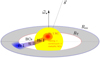 |
Fig. 21 Schematic picture of the circumstellar environment of RU Lup. ω* and ŝ are the stellar rotation axis and the line of sight to the observer, respectively. |
Acknowledgements
The authors thank the anonymous referee for their review of this manuscript. This work has been supported by Deutsche Forschungsgemeinschaft (DFG) in the framework of the YTTHACA Project (469334657) under the project codes STE 1068/9-1 and MA 8447/1-1. PCS acknowledges support from DLR 50 OR 2205. AF, EF, and JMA acknowledge financial support from the project PRIN-INAF 2019 “Spectroscopically Tracing the Disk Dispersal Evolution” (STRADE) and the Large Grant INAF 2022 “YSOs Outflows, Disks and Accretion: towards a global framework for the evolution of planet forming systems” (YODA). CFM and JCW are funded by the European Union (ERC, WANDA, 101039452). Views and opinions expressed are however those of the author(s) only and do not necessarily reflect those of the European Union or the European Research Council Executive Agency. Neither the European Union nor the granting authority can be held responsible for them. JFG was supported by Fundação para a Ciência e Tecnologia (FCT) through the research grants UIDB/04434/2020 and UIDP/04434/2020. This work benefited from discussions with the ODYSSEUS team6 (HST AR-16129). Observing time with Chiron was awarded through NOIRLab programs 2022a-492217, 2022B-994458, and 2023A-579477 (PI FMW). Chiron is operated by the SMARTS Consortium. Funding for the TESS mission is provided by NASA’s Science Mission directorate. The authors acknowledge Thomas Sperling, Michael Siwak, Ignacio Mendigutía, Konstantin Grankin, Rebeca Garcia López, and Jerome Bouvier for comments and suggestions on this work. The authors acknowledge with thanks the variable star observations from the AAVSO International Database contributed by observers worldwide and used in this research, and Elizabeth Waagen for coordinating the AAVSO Alerts. The authors acknowledge the use of the electronic bibliography maintained by the NASA/ADS7 system.
Appendix A Log of spectroscopic observations
Table A.1 reports the log of the spectroscopic observations.
Log of the spectroscopic observations.
Appendix B Gaussian fits
We used a multiple Gaussian model to fit the continuum-normalized emission lines in the spectrum of RU Lup. This model is a sum of symmetric (S) and asymmetric (A) Gaussian functions. The asymmetric Gaussian function 𝒢A is defined as
![Mathematical equation: $\[\mathcal{G}_{\mathrm{A}}(v)=C \exp \left[-\frac{\left(v-v_0\right)^2}{2 \sigma^2}\right] \text {, with } \sigma= \begin{cases}\sigma_{\mathrm{b}} & \text { if } v<v_0 \\ \sigma_{\mathrm{r}} & \text { if } v \geq v_0\end{cases}\]$](/articles/aa/full_html/2024/10/aa51065-24/aa51065-24-eq31.png) (B.1)
(B.1)
where C is the amplitude relative to the continuum, v0 is the line center and σ, σb, and σr are standard deviations. The symmetric Gaussian function 𝒢S has σb = σr. The model is called nS+mA in the main text, where n and m are the number of symmetric and asymmetric Gaussian functions, respectively. It is expressed as
![Mathematical equation: $\[F(v)=1+\sum_{i=1}^n \mathcal{G}_{\mathrm{Si}}(v)+\sum_{i=1}^m \mathcal{G}_{\mathrm{Ai}}(v).\]$](/articles/aa/full_html/2024/10/aa51065-24/aa51065-24-eq32.png) (B.2)
(B.2)
Appendix C Calculation of continuum veiling
We estimated the veiling in our spectra using the ES 22.5 observation as template, which is the spectrum with the highest S/N among the ones with lower veiling in our sample. This method simplifies the calculation of the veiling, because the template does not have to be rotationally broadened. In addition, there are epochs in which the line-filling emission is so strong that the fit with ROTFIT did not converge allowing v sin i to vary (e.g., ES 21.1).
The veiling of the spectra relative to the ES 22.5 template (VFrel) is defined as VFrel = [Fobs(λ) − FT(λ)]/FT,c, where Fobs(λ) and FT(λ) are the observed and template spectra and FT,c is the continuum of the template. VFrel can be converted to the absolute veiling; that is the veiling with respect to that of a hypothetical spectrum of RU Lup if it did not exhibit any accretion. The absolute veiling is VFabs = [Fobs(λ) − F0(λ)]/F0,c where F0(λ) and F0,c is the wavelength-dependent flux of the non-accreting version of RULup and its continuum, respectively. VFabs can be determined because the absolute veiling VFT of the template could be computed independently with ROTFIT (Sec. 3). Since VFT is defined as VFT = [FT(λ) − F0(λ)]/F0,c, and this relation also holds for the continua – that is, VFT = [FT,c − F0,c]/F0,c – it can be shown that the equation for the conversion is
![Mathematical equation: $\[1+\mathrm{VF}_{\mathrm{abs}}=\left(1+\mathrm{VF}_{\text {rel }}\right) \cdot\left(1+\mathrm{VF}_{\mathrm{T}}\right).\]$](/articles/aa/full_html/2024/10/aa51065-24/aa51065-24-eq33.png) (C.1)
(C.1)
We computed the veiling in the two spectral regions shown in Fig. 2. We define the veiling in these two regions as VF5735 and VF5800. For both regions, we used VFT = 1.57 ± 0.31 for the ES 22.5 spectrum. The procedure to estimate VFrel consisted of the following steps:
normalization of the spectra with a linear fit of selected portions of the spectrum where the continuum is seen;
down-grading of the template to the resolution of the observed spectrum;
cross-correlation between the template and the observation to match the position of the absorption lines;
exclusion of regions affected by line emission;
-
computation of the χ2-function, defined as
![Mathematical equation: $\[\chi^2\left(\mathrm{VF}_{\text {rel }}\right)=\sum_{\lambda_{\mathrm{i}}}\left(\mathrm{~F}_{\text {obs }}\left(\lambda_{\mathrm{i}}\right)-\frac{\mathrm{F}_{\mathrm{T}}\left(\lambda_{\mathrm{i}}\right)+\mathrm{VF}_{\text {rel }}}{1+\mathrm{VF}_{\text {rel }}}\right)^2\]$](/articles/aa/full_html/2024/10/aa51065-24/aa51065-24-eq34.png) (C.2)
(C.2)as a function of VFrel.
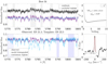 |
Fig. C.1 Veiling calculation for the ES 21.1 spectrum. The bottom left panel shows the ES 21.1 and ES 22.5 spectra, normalized used the shaded regions. The top left panel shows the veiled ES 22.5 spectrum that best fits the ES 21.1 spectrum. The right panels display the cross correlation function (bottom) and the χ2 as a function of VF (top). |
The best fitting VFrel was found minimizing the χ2, and the uncertainty as the standard deviation of exp(−χ2). Then, we converted VFrel to VFabs using Eq. C.1.
Figure C.1 shows the procedure to compute VF5800 for the ES 21.1 spectrum, pointing out the effect of line emission in the estimation of the VF. Due to the resolution, the S/N, and the effect of line emission, sometimes the fits did not converge. Therefore, we selected the observations for which VF5735 and VF5800 differed by more than 1σ, we visually inspected the results of the procedure for both regions, and we excluded the cases that we considered unclear. When both VF5735 and VF5800 agreed with each other, we derived a single measure of VFabs by computing a weighted average (with weights ![Mathematical equation: $\[w_i=1 / d \mathrm{VF}_{\mathrm{i}}^2\]$](/articles/aa/full_html/2024/10/aa51065-24/aa51065-24-eq35.png) ) of the two values. The results are reported in Table A.1.
) of the two values. The results are reported in Table A.1.
Appendix D Spot model
We derived an analytical model to reproduce the variability of the TESS light curve. We assumed a spot with a constant temperature T, filling factor f, located at a latitude θS and azimuth ϕ on the surface of the star. The spot radiates as a black-body: its energy per unit time, area, solid angle, and wavelength interval is given by
![Mathematical equation: $\[B_\lambda(T)=\frac{2 h c^5}{\lambda^5} \frac{1}{\exp \left(h c / k_{\mathrm{B}} T\right)-1},\]$](/articles/aa/full_html/2024/10/aa51065-24/aa51065-24-eq36.png) (D.1)
(D.1)
where h is the Plank constant, c is the speed of light, kB is the Boltzmann constant, and λ is the wavelength. The projected surface of the spot varies as
![Mathematical equation: $\[S(\phi)=S_0(\hat{n} \cdot \hat{s}),\]$](/articles/aa/full_html/2024/10/aa51065-24/aa51065-24-eq37.png) (D.2)
(D.2)
where ![Mathematical equation: $\[S_0=4 \pi R_{\star}^2 f\]$](/articles/aa/full_html/2024/10/aa51065-24/aa51065-24-eq38.png) is the surface of the spot,
is the surface of the spot, ![Mathematical equation: $\[\hat{n}=\left(\cos \theta_{\mathrm{S}} \cos \phi, \cos \theta_{\mathrm{S}} \sin \phi, \sin \theta_{\mathrm{S}}\right)\]$](/articles/aa/full_html/2024/10/aa51065-24/aa51065-24-eq39.png) is the normal to the surface, and ŝ = (sin i, 0, cos i) is the line of sight toward an observer located at an angle i from the rotation axis. Therefore, the flux observed with TESS is
is the normal to the surface, and ŝ = (sin i, 0, cos i) is the line of sight toward an observer located at an angle i from the rotation axis. Therefore, the flux observed with TESS is
![Mathematical equation: $\[\begin{aligned}F\left(T, f, \theta_{\mathbf{S}}, \phi\right)=F_{\star}+\left[\frac{R_{\star}^2}{d^2} f ~\int~ B_\lambda(T) R(\lambda) d \lambda\right]\quad\qquad\quad \\\cdot\left(\cos \theta_{\mathrm{S}} \sin i \cos \phi+\sin \theta_{\mathrm{S}} \cos i\right)\end{aligned}\]$](/articles/aa/full_html/2024/10/aa51065-24/aa51065-24-eq40.png) (D.3)
(D.3)
where d is the distance to the system, R(λ) is the response function of the TESS filter, and
![Mathematical equation: $\[F_{\star}=\frac{R_{\star}^2}{2 d^2} \int B_\lambda\left(T_{\text {eff }}\right) R(\lambda) d \lambda=2.7 \times 10^{-14} ~\mathrm{erg} \mathrm{~s}^{-1} \mathrm{~cm}^{-2}\]$](/articles/aa/full_html/2024/10/aa51065-24/aa51065-24-eq41.png) (D.4)
(D.4)
is the integrated flux of the star in the TESS bandpass8. We downloaded the TESS response function from the SVO Filter Profile Service9 (Rodrigo & Solano 2020). The modulation can be written as
![Mathematical equation: $\[F\left(T, f, \theta_S, \phi\right)=F_{\star}+A \cos \phi+C.\]$](/articles/aa/full_html/2024/10/aa51065-24/aa51065-24-eq42.png) (D.5)
(D.5)
with
![Mathematical equation: $\[A=\left[\frac{R_{\star}^2}{d^2} f \int B_\lambda(T) R(\lambda) d \lambda\right] \cos \theta_{\mathrm{S}} \sin i\]$](/articles/aa/full_html/2024/10/aa51065-24/aa51065-24-eq43.png) (D.6)
(D.6)
and
![Mathematical equation: $\[C=A \frac{\tan \theta_{\mathrm{s}}}{\tan i}.\]$](/articles/aa/full_html/2024/10/aa51065-24/aa51065-24-eq44.png) (D.7)
(D.7)
The latitude of the spot can be directly obtained from the inversion of Eq. D.7, while from the amplitude A of the oscillations we get a relation between f and T
![Mathematical equation: $\[f=A \frac{d^2}{R_{\star}^2}\left[\int B_\lambda(T) R(\lambda) d \lambda\right]^{-1}\left(\cos \theta_{\mathrm{S}} \sin i\right)^{-1}.\]$](/articles/aa/full_html/2024/10/aa51065-24/aa51065-24-eq45.png) (D.8)
(D.8)
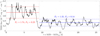 |
Fig. D.1 TESS Sector 65 light curve converted in absolute flux in the TESS bandpass. The solid lines mark the zero point of the oscillations, while the dotted lines mark the maximum and the minimum of the oscillations. The vertical dashed lines indicate the transition between the two portions. FC and FA are the zero point and the amplitude fluxes, respectively, in units of 10−13 erg s−1 cm−2. |
We converted the TESS magnitude T to flux F using the formula F = ZPλ 10−T/2.5, where ZPλ = 1.33 × 10⁻⁹ erg s−1 cm−2 is the zero point flux of TESS, that we took from the SVO Filter Profile Service. Then, we visually estimated the amplitude FA and the zero point FC of the oscillations for the two portions of the light curve, defined as in Sec. 6. The values are reported in Fig. D.1. The latitude of the spot and the relation between f and T can be derived from Eqs. D.7 and D.8 with C = FC − F* and A = FA. We derived θS1 = 61° and θS2 = 65° for the latitude of the spot in the two segments. The relation between f and T (Eq. D.8) is shown in Fig. 17.
Appendix E Filling factor of a spherical cap
A spherical cap is a portion of a sphere cut by a plane. In spherical coordinates, it is defined as
![Mathematical equation: $\[\left\{(\theta, \phi) \quad \left\lvert\, \quad \frac{\pi}{2}-\Delta \theta_{\mathrm{S}} \leq \theta \leq \frac{\pi}{2}\right., \quad 0 \leq \phi \leq 2 \pi\right\}\]$](/articles/aa/full_html/2024/10/aa51065-24/aa51065-24-eq46.png) (E.1)
(E.1)
where θ and ϕ are the latitude and the azimuth, and ΔθS is the half-aperture angle of the cap (spot). The filling factor of the cap can be computed by integrating
![Mathematical equation: $\[f=\frac{1}{4 \pi R_{\star}^2} \int_{\pi / 2-\Delta \theta_{\mathrm{S}}}^{\pi / 2} \int_0^{2 \pi} R_{\star}^2 \cos \theta d \theta d \phi=\frac{1}{2}\left(1-\cos \Delta \theta_{\mathrm{S}}\right).\]$](/articles/aa/full_html/2024/10/aa51065-24/aa51065-24-eq47.png) (E.2)
(E.2)
Inverting this relation, we obtain
![Mathematical equation: $\[\Delta \theta_{\mathrm{S}}=\arccos ~(1-2 f).\]$](/articles/aa/full_html/2024/10/aa51065-24/aa51065-24-eq48.png) (E.3)
(E.3)
References
- Alcalá, J. M., Manara, C. F., Natta, A., et al. 2017, A&A, 600, A20 [NASA ADS] [CrossRef] [EDP Sciences] [Google Scholar]
- Alencar, S. H. P., Bouvier, J., Walter, F. M., et al. 2012, A&A, 541, A116 [NASA ADS] [CrossRef] [EDP Sciences] [Google Scholar]
- Ardila, D. R., Herczeg, G. J., Gregory, S. G., et al. 2013, ApJS, 207, 1 [NASA ADS] [CrossRef] [Google Scholar]
- Armeni, A., Stelzer, B., Claes, R. A. B., et al. 2023, A&A, 679, A14 [NASA ADS] [CrossRef] [EDP Sciences] [Google Scholar]
- Azevedo, R., Calvet, N., Hartmann, L., et al. 2006, A&A, 456, 225 [NASA ADS] [CrossRef] [EDP Sciences] [Google Scholar]
- Beristain, G., Edwards, S., & Kwan, J. 1998, ApJ, 499, 828 [NASA ADS] [CrossRef] [Google Scholar]
- Beristain, G., Edwards, S., & Kwan, J. 2001, ApJ, 551, 1037 [Google Scholar]
- Blinova, A. A., Romanova, M. M., & Lovelace, R. V. E. 2016, MNRAS, 459, 2354 [Google Scholar]
- Bouvier, J., Alencar, S. H. P., Boutelier, T., et al. 2007a, A&A, 463, 1017 [NASA ADS] [CrossRef] [EDP Sciences] [Google Scholar]
- Bouvier, J., Alencar, S. H. P., Harries, T. J., Johns-Krull, C. M., & Romanova, M. M. 2007b, in Protostars and Planets V, eds. B. Reipurth, D. Jewitt, & K. Keil, 479 [Google Scholar]
- Calvet, N., & Gullbring, E. 1998, ApJ, 509, 802 [Google Scholar]
- Calvet, N., & Hartmann, L. 1992, ApJ, 386, 239 [CrossRef] [Google Scholar]
- Calvet, N., Muzerolle, J., Briceño, C., et al. 2004, AJ, 128, 1294 [NASA ADS] [CrossRef] [Google Scholar]
- Campbell-White, J., Sicilia-Aguilar, A., Manara, C. F., et al. 2021, MNRAS, 507, 3331 [NASA ADS] [CrossRef] [Google Scholar]
- Dekker, H., D’Odorico, S., Kaufer, A., Delabre, B., & Kotzlowski, H. 2000, SPIE Conf. Ser., 4008, 534 [Google Scholar]
- Dodin, A. V., & Lamzin, S. A. 2012, Astron. Lett., 38, 649 [Google Scholar]
- Espaillat, C. C., Robinson, C. E., Romanova, M. M., et al. 2021, Nature, 597, 41 [NASA ADS] [CrossRef] [Google Scholar]
- Espaillat, C. C., Herczeg, G. J., Thanathibodee, T., et al. 2022, AJ, 163, 114 [NASA ADS] [CrossRef] [Google Scholar]
- Frasca, A., Biazzo, K., Lanzafame, A. C., et al. 2015, A&A, 575, A4 [NASA ADS] [CrossRef] [EDP Sciences] [Google Scholar]
- Frasca, A., Biazzo, K., Alcalá, J. M., et al. 2017, A&A, 602, A33 [NASA ADS] [CrossRef] [EDP Sciences] [Google Scholar]
- Gahm, G. F., Walter, F. M., Stempels, H. C., Petrov, P. P., & Herczeg, G. J. 2008, A&A, 482, L35 [NASA ADS] [CrossRef] [EDP Sciences] [Google Scholar]
- Gaia Collaboration (Brown, A. G. A., et al.) 2021, A&A, 649, A1 [NASA ADS] [CrossRef] [EDP Sciences] [Google Scholar]
- GRAVITY Collaboration (Perraut, K., et al.) 2021, A&A, 655, A73 [NASA ADS] [CrossRef] [EDP Sciences] [Google Scholar]
- Hartigan, P., Hartmann, L., Kenyon, S., Hewett, R., & Stauffer, J. 1989, ApJS, 70, 899 [NASA ADS] [CrossRef] [Google Scholar]
- Hartmann, L., Herczeg, G., & Calvet, N. 2016, ARA&A, 54, 135 [Google Scholar]
- Herbig, G. H. 1962, A&A, 1, 47 [NASA ADS] [Google Scholar]
- Herczeg, G. J., Walter, F. M., Linsky, J. L., et al. 2005, AJ, 129, 2777 [NASA ADS] [CrossRef] [Google Scholar]
- Herczeg, G. J., Chen, Y., Donati, J.-F., et al. 2023, ApJ, 956, 102 [NASA ADS] [CrossRef] [Google Scholar]
- Horne, K., & Marsh, T. R. 1986, MNRAS, 218, 761 [NASA ADS] [CrossRef] [Google Scholar]
- Johnstone, R. M., & Penston, M. V. 1986, MNRAS, 219, 927 [CrossRef] [Google Scholar]
- Joy, A. H. 1945, ApJ, 102, 168 [Google Scholar]
- Kulkarni, A. K., & Romanova, M. M. 2008, MNRAS, 386, 673 [Google Scholar]
- Kulkarni, A. K., & Romanova, M. M. 2009, MNRAS, 398, 701 [Google Scholar]
- Kulkarni, A. K., & Romanova, M. M. 2013, MNRAS, 433, 3048 [NASA ADS] [CrossRef] [Google Scholar]
- Lamzin, S. A. 1999, Astron. Lett., 25, 430 [NASA ADS] [Google Scholar]
- Lomb, N. R. 1976, Ap&SS, 39, 447 [Google Scholar]
- Manara, C. F., Frasca, A., Venuti, L., et al. 2021, A&A, 650, A196 [NASA ADS] [CrossRef] [EDP Sciences] [Google Scholar]
- Manara, C. F., Ansdell, M., Rosotti, G. P., et al. 2023, in Protostars and Planets VII, 534, eds. S. Inutsuka, Y. Aikawa, T. Muto, K. Tomida, & M. Tamura, 539 [Google Scholar]
- Mayor, M., Pepe, F., Queloz, D., et al. 2003, The Messenger, 114, 20 [NASA ADS] [Google Scholar]
- McGinnis, P., Bouvier, J., & Gallet, F. 2020, MNRAS, 497, 2142 [Google Scholar]
- Muzerolle, J., Hartmann, L., & Calvet, N. 1998, AJ, 116, 455 [Google Scholar]
- Pantolmos, G., Zanni, C., & Bouvier, J. 2020, A&A, 643, A129 [NASA ADS] [CrossRef] [EDP Sciences] [Google Scholar]
- Pepe, F., Cristiani, S., Rebolo, R., et al. 2021, A&A, 645, A96 [NASA ADS] [CrossRef] [EDP Sciences] [Google Scholar]
- Percy, J. R., Esteves, S., Glasheen, J., et al. 2010, JAAVSO, 38, 151 [NASA ADS] [Google Scholar]
- Petrov, P. P., Gahm, G. F., Gameiro, J. F., et al. 2001, A&A, 369, 993 [NASA ADS] [CrossRef] [EDP Sciences] [Google Scholar]
- Petrov, P. P., Gahm, G. F., Stempels, H. C., Walter, F. M., & Artemenko, S. A. 2011, A&A, 535, A6 [NASA ADS] [CrossRef] [EDP Sciences] [Google Scholar]
- Rei, A. C. S., Petrov, P. P., & Gameiro, J. F. 2018, A&A, 610, A40 [NASA ADS] [CrossRef] [EDP Sciences] [Google Scholar]
- Ricker, G. R., Winn, J. N., Vanderspek, R., et al. 2014, SPIE Conf. Ser., 9143, 914320 [Google Scholar]
- Rodrigo, C., & Solano, E. 2020, in XIV.0 Scientific Meeting of the Spanish Astronomical Society, 182 [Google Scholar]
- Roman-Duval, J., Proffitt, C. R., Taylor, J. M., et al. 2020, RNAAS, 4, 205 [NASA ADS] [Google Scholar]
- Romanova, M. M., & Kulkarni, A. K. 2009, MNRAS, 398, 1105 [CrossRef] [Google Scholar]
- Romanova, M. M., & Owocki, S. P. 2015, Space Sci. Rev., 191, 339 [Google Scholar]
- Romanova, M. M., Ustyugova, G. V., Koldoba, A. V., Wick, J. V., & Lovelace, R. V. E. 2003, ApJ, 595, 1009 [Google Scholar]
- Romanova, M. M., Ustyugova, G. V., Koldoba, A. V., & Lovelace, R. V. E. 2004, ApJ, 610, 920 [Google Scholar]
- Sacco, G. G., Argiroffi, C., Orlando, S., et al. 2008, A&A, 491, L17 [NASA ADS] [CrossRef] [EDP Sciences] [Google Scholar]
- Scargle, J. D. 1982, ApJ, 263, 835 [Google Scholar]
- Sicilia-Aguilar, A., Kóspál, Á., Setiawan, J., et al. 2012, A&A, 544, A93 [NASA ADS] [CrossRef] [EDP Sciences] [Google Scholar]
- Sicilia-Aguilar, A., Fang, M., Roccatagliata, V., et al. 2015, A&A, 580, A82 [NASA ADS] [CrossRef] [EDP Sciences] [Google Scholar]
- Sicilia-Aguilar, A., Campbell-White, J., Roccatagliata, V., et al. 2023, MNRAS, 526, 4885 [NASA ADS] [CrossRef] [Google Scholar]
- Siwak, M., Ogloza, W., Rucinski, S. M., et al. 2016, MNRAS, 456, 3972 [NASA ADS] [CrossRef] [Google Scholar]
- Smette, A., Sana, H., Noll, S., et al. 2015, A&A, 576, A77 [NASA ADS] [CrossRef] [EDP Sciences] [Google Scholar]
- Stempels, H. C., Gahm, G. F., & Petrov, P. P. 2007, A&A, 461, 253 [NASA ADS] [CrossRef] [EDP Sciences] [Google Scholar]
- Stock, C., McGinnis, P., Caratti o Garatti, A., Natta, A., & Ray, T. P. 2022, A&A, 668, A94 [NASA ADS] [CrossRef] [EDP Sciences] [Google Scholar]
- Tokovinin, A., Fischer, D. A., Bonati, M., et al. 2013, PASP, 125, 1336 [NASA ADS] [CrossRef] [Google Scholar]
- Vanderspek, R., Doty, J. P., Fausnaugh, M., et al. 2018, TESS Instrument Handbook [Google Scholar]
- Vernet, J., Dekker, H., D’Odorico, S., et al. 2011, A&A, 536, A105 [NASA ADS] [CrossRef] [EDP Sciences] [Google Scholar]
- Wendeborn, J., Espaillat, C. C., Lopez, S., et al. 2024a arXiv e-prints [arXiv:2405.21038] [Google Scholar]
- Wendeborn, J., Espaillat, C. C., Thanathibodee, T., et al. 2024b arXiv e-prints [arXiv:2405.21071] [Google Scholar]
- Wilson, T. J. G., Matt, S., Harries, T. J., & Herczeg, G. J. 2022, MNRAS, 514, 2162 [NASA ADS] [CrossRef] [Google Scholar]
We used this spectrum because it is the only one that is absolutely flux-calibrated among the CHIRON spectra from 2023.
This derivation has the subtlety that the spectroscopic estimate of ![Mathematical equation: $\[\dot{M}_{\mathrm{acc}}\]$](/articles/aa/full_html/2024/10/aa51065-24/aa51065-24-eq49.png) depends in turn on RT.
depends in turn on RT.
The factor 1/2 comes from the fact that we see only one hemisphere.
All Tables
All Figures
|
Fig. 1 AAVSO B (blue) and V (green) photometry contemporaneous to the spectroscopic observations in 2021 and 2022. The vertical dashed lines mark the epochs of the CHIRON (black) and ESPRESSO (red) observations. The ES 21.1 and ES 22.5 spectra shown in Fig. 2 are marked in violet and light blue. Here, MJD0 ≡ 59264.336. |
| In the text | |
|
Fig. 2 ES 21.1 and ES 22.5 spectra in two regions where the photospheric absorption lines are observed. The region between 5770 and 5805 Å shows the effect of line-filling emission. |
| In the text | |
|
Fig. 3 Best fit of the He I 5876 line in ES 21.1 with two different models. Both models use three Gaussian functions. In the left panel, the Gaussian for the NC is symmetric, while in the right panel it has two different σ. See Appendix B for details on the model. The single components are marked with dashed lines, with the blue one indicating the Gaussian for the NC. The insets are a zoom on the NC. |
| In the text | |
|
Fig. 4 Lomb Scargle Periodogram of the radial velocity of the He I 5876 NC. |
| In the text | |
|
Fig. 5 Phase-folded radial velocity curve of the He I 5876 NC. The red line is the best fit with a sinusoidal function. |
| In the text | |
|
Fig. 6 Selection of emission lines that have a NC. The light blue spectrum is ES 22.5. The dark blue spectra are the template that best fits the stellar spectrum (Sec. 3), veiled to match the depth of the photo-spheric lines. The photospheric subtracted spectra are shown in black, with Gaussian best fits superposed in red. The red label specifies the multiple Gaussian model used (Appendix B). |
| In the text | |
|
Fig. 7 Anti-phase radial velocity variations of the He I 5876 NC (red) and the photospheric lines (black) in the ESPRESSO spectra. R is the Pearson correlation coefficient between vphot and vNC. |
| In the text | |
|
Fig. 8 Flux-subtraction of the ES 22.5 spectrum from the other ESPRESSO spectra. The top panel shows the five subtracted spectra median filtered to three points. ES 22.5 is shown in the bottom panel for reference. |
| In the text | |
|
Fig. 9 Comparison between the ES 21.1 and ES 22.5 spectra in regions dominated by metallic emission lines. Species producing line emission are marked. The Fe I 5447, Si II 6347, and Ca I 6122 lines used in Sec. 6.1 are marked in red. |
| In the text | |
|
Fig. 10 Continuum subtracted profiles of the Fe II 5317, He I 6678, Si II 6347, and Fe I 5447 lines in the ESPRESSO spectra. |
| In the text | |
|
Fig. 11 Subtraction between consecutive Fe II 5317 ESPRESSO spectra. The color code is the same as in Fig. 10. The profiles were rescaled by a constant (upper right corner). The bottom panels show the subtracted profiles, with Gaussian fits superposed. |
| In the text | |
|
Fig. 12 Relation between vBC and LA for the He I 6678, Si II 6347, and Fe I 5447 lines. R is the Pearson correlation coefficient. |
| In the text | |
|
Fig. 13 Selected observations showing the variability of the asymmetry of the He I 6678, Si II 6347, and Fe I 5447 lines. Here, LA is the line asymmetry to the blue. |
| In the text | |
|
Fig. 14 TESS light curve of RU Lup from Sector 65 (2023). The light curve is plotted as a function of the time t from the beginning of the observation (MJDbeg = 60068.25). The top axis show the phase ϕ computed with P = 3.63 days (i.e., the spot period, Sec. 4.1). The reference date for ϕ = 0 is MJD0 ≡ 59264.336. The blue lines mark the phase ϕS (from Sec. 4.1), where the maximum contribution from the hot spot is expected. The red lines mark the epochs of the CHIRON spectroscopic observations. |
| In the text | |
|
Fig. 15 Continuous wavelet analysis of the TESS Sector 65 light curve. The top panel shows the CWT. The bottom panel displays the light curve. The insets show the LSP for the two portions of the light curve. The blue and red lines mark the detected period and P*, respectively. Sinusoidal oscillations are superposed to the TESS observation in green, with the period of the oscillations in each portion reported with the same color. |
| In the text | |
|
Fig. 16 Normalized profiles of the Fe I 5447, Si II 6347, and Ca I 6122 lines in the 9 CHIRON spectra that are contemporaneous to the TESS Sector 65 light curve. Tmag is the TESS magnitude at these epochs. |
| In the text | |
|
Fig. 17 Relation between the filling factor (f) and the temperature (T) (Appendix D), for a spot that reproduces the modulations observed in the TESS Sector 65 light curve. The gray area marks 0.18 ≤ f ≤ 0.26 (Wendeborn et al. 2024a), while the dashed line marks f = 0.12 (Dodin & Lamzin 2012). |
| In the text | |
|
Fig. 18 Sketch of the possible vertical stratification of the hot spot inferred from the analysis of the NCs. vpre and vpost are the pre-shock and post-shock velocities. |
| In the text | |
|
Fig. 19 Radial velocity curve of the He I 5876 NC for the 2022 observations only. The inset shows the LSP, with the detected P and P* marked with dashed blue and red lines, respectively. |
| In the text | |
|
Fig. 20 A selection of metallic lines in the spectra of RU Lup, HM Lup, and Sz 98. |
| In the text | |
|
Fig. 21 Schematic picture of the circumstellar environment of RU Lup. ω* and ŝ are the stellar rotation axis and the line of sight to the observer, respectively. |
| In the text | |
|
Fig. C.1 Veiling calculation for the ES 21.1 spectrum. The bottom left panel shows the ES 21.1 and ES 22.5 spectra, normalized used the shaded regions. The top left panel shows the veiled ES 22.5 spectrum that best fits the ES 21.1 spectrum. The right panels display the cross correlation function (bottom) and the χ2 as a function of VF (top). |
| In the text | |
|
Fig. D.1 TESS Sector 65 light curve converted in absolute flux in the TESS bandpass. The solid lines mark the zero point of the oscillations, while the dotted lines mark the maximum and the minimum of the oscillations. The vertical dashed lines indicate the transition between the two portions. FC and FA are the zero point and the amplitude fluxes, respectively, in units of 10−13 erg s−1 cm−2. |
| In the text | |
Current usage metrics show cumulative count of Article Views (full-text article views including HTML views, PDF and ePub downloads, according to the available data) and Abstracts Views on Vision4Press platform.
Data correspond to usage on the plateform after 2015. The current usage metrics is available 48-96 hours after online publication and is updated daily on week days.
Initial download of the metrics may take a while.