| Issue |
A&A
Volume 690, October 2024
|
|
|---|---|---|
| Article Number | A76 | |
| Number of page(s) | 14 | |
| Section | Extragalactic astronomy | |
| DOI | https://doi.org/10.1051/0004-6361/202450746 | |
| Published online | 02 October 2024 | |
VLTI/GRAVITY interferometric measurements of the innermost dust structure sizes around active galactic nuclei⋆
1
Universidade de Lisboa – Faculdade de Ciências, Campo Grande, 1749-016 Lisboa, Portugal
2
CENTRA – Centro de Astrofísica e Gravitação, IST, Universidade de Lisboa, 1049-001 Lisboa, Portugal
3
Max Planck Institute for Extraterrestrial Physics (MPE), Giessenbachstr. 1, 85748 Garching, Germany
4
Max Planck Institute for Astronomy, Königstuhl 17, 69117 Heidelberg, Germany
5
LESIA, Observatoire de Paris, Université PSL, CNRS, Sorbonne Université, Univ. Paris Diderot, Sorbonne Paris Cité, 5 Place Jules Janssen, 92195 Meudon, France
6
Leiden University, 2311 EZ Leiden, The Netherlands
7
Department of Astrophysical & Planetary Sciences, JILA, University of Colorado, Duane Physics Bldg. 2000 Colorado Ave, Boulder, CO 80309, USA
8
I. Institute of Physics, University of Cologne, Zülpicher Straße 77, 50937 Cologne, Germany
9
Max Planck Institute for Radio Astronomy, Auf dem Hügel 69, 53121 Bonn, Germany
10
European Southern Observatory, Alonso de Córdova 3107, Casilla, 19001 Vitacura, Santiago, Chile
11
Faculdade de Engenharia, Universidade do Porto, Rua Dr. Roberto Frias, 4200-465 Porto, Portugal
12
Departments of Physics and Astronomy, Le Conte Hall, University of California, Berkeley, CA 94720, USA
13
Research School of Astronomy and Astrophysics, Australian National University, Canberra, ACT 2611, Australia
14
Department of Physics and Astronomy, University of Southampton, Southampton, UK
15
Department of Astrophysics & Atmospheric Sciences, Kyoto Sangyo University, Kamigamo-motoyama, Kita-ku, Kyoto 603-8555, Japan
16
European Southern Observatory, Karl-Schwarzschild-Str. 2, 85748 Garching, Germany
17
Université Côte d’Azur, Observatoire de la Côte d’Azur, CNRS, Laboratoire Lagrange, Nice, France
18
School of Physics and Astronomy, Tel Aviv University, Tel Aviv 69978, Israel
19
Univ. Grenoble Alpes, CNRS, IPAG, 38000 Grenoble, France
20
Retired – c/o T.L. Turner, 205 South Prospect Street, Granville, OH 43023, USA
21
Instituto de Astrofísica de Canarias (IAC), E-38205 La Laguna, Tenerife, Spain
22
Center for Computational Astrophysics, Flatiron Institute, 162 5th Ave., New York, NY 10010, USA
Received:
16
May
2024
Accepted:
18
July
2024
Abstract
We present new Very Large Telescope Interferometer (VLTI)/GRAVITY near-infrared interferometric measurements of the angular size of the innermost hot dust continuum for 14 type 1 active galactic nuclei (AGNs). The angular sizes are resolved on scales of ∼0.7 mas and the inferred ring radii range from 0.028 to 1.33 pc, comparable to those reported previously and a factor of 10−20 smaller than the mid-infrared sizes in the literature. Combining our new data with previously published values, we compiled a sample of 25 AGNs with bolometric luminosity ranging from 1042 to 1047 erg s−1, with which we studied the radius-luminosity (R − L) relation for the hot dust structure. Our interferometric measurements of radius are offset by a factor of 2 from the equivalent relation derived through reverberation mapping. Using a simple model to explore the dust structure’s geometry, we conclude that this offset can be explained if the 2 μm emitting surface has a concave shape. Our data show that the slope of the relation is in line with the canonical R ∝ L0.5 when using an appropriately non-linear correction for bolometric luminosity. In contrast, using optical luminosity or applying a constant bolometric correction to it results in a significant deviation in the slope, suggesting a potential luminosity dependence on the spectral energy distribution. Over four orders of magnitude in luminosity, the intrinsic scatter around the R − L relation is 0.2 dex, suggesting a tight correlation between the innermost hot dust structure size and the AGN luminosity.
Key words: techniques: interferometric / galaxies: active / galaxies: nuclei / galaxies: Seyfert
GRAVITY is developed in a collaboration by the Max Planck Institute for Extraterrestrial Physics, LESIA of Observatoire de Paris/Université PSL/CNRS/Sorbonne Université/Université de Paris and IPAG of Université Grenoble Alpes/CNRS, the Max Planck Institute for Astronomy, the University of Cologne, the CENTRA – Centro de Astrofisicae Gravitação, and the European Southern Observatory.
Corresponding authors; This email address is being protected from spambots. You need JavaScript enabled to view it. , This email address is being protected from spambots. You need JavaScript enabled to view it.
© The Authors 2024
 Open Access article, published by EDP Sciences, under the terms of the Creative Commons Attribution License (https://creativecommons.org/licenses/by/4.0), which permits unrestricted use, distribution, and reproduction in any medium, provided the original work is properly cited.
This article is published in open access under the Subscribe to Open model.
Open Access funding provided by Max Planck Society.
1. Introduction
The central engine of an active galactic nucleus (AGN) is powered by accretion onto a supermassive black hole (SMBH) with a mass that can be in the range from ∼105 M⊙ in dwarf galaxies (Baldassare et al. 2015; Reines 2022; Mezcua & Sánchez 2024) to ∼1010 M⊙ in the most massive galaxies (McConnell et al. 2011; Mehrgan et al. 2019). The UV photons from the accretion disk (Shakura & Sunyaev 1973) ionise the gas in its close proximity, forming the broad line region (BLR). Dust sublimates on these scales (Barvainis 1987), but is an important component further out because of the key observational impact it has. It is found in disk, outflow, and filament structures in the innermost region surrounding the AGN, and is responsible for significant nuclear obscuration (Antonucci & Miller 1985; Urry & Padovani 1995; Hönig 2019; Prieto et al. 2021). Much of the progress in our understanding of these inner structures of AGNs has come about through substantial improvements in observational techniques (Netzer 2015). Notably, mid-infrared (MIR) and near-infrared (NIR) interferometry, here referred to as optical/infrared interferometry (OI), enables one to spatially resolve subparsec scales even in distant objects, and is opening new opportunities for studies of AGNs.
Long-baseline infrared interferometry has made it possible to delve into the detailed structure of dust by resolving its thermal emission at different wavelengths. At MIR wavelengths, interferometric observations of AGNs has resolved warm dust structures emitting at a typical temperature of 400 K on scales of 3–30 mas (Kishimoto et al. 2011a; Burtscher et al. 2013). Contrary to the classical torus model, detailed modelling of the data has revealed a significant fraction of the total flux coming, in many sources, from the polar region containing graphite grain dust on parsec or larger scales (Hönig et al. 2013; López-Gonzaga et al. 2016; Leftley et al. 2018).
An alternate approach for investigating the dust structure is to monitor the time delay between the optical and NIR continuum emission. Using the time delay as an indicator of size, this reverberation mapping (RM) technique has measured the sizes of hot dust structures for ∼30 AGNs (e.g. Clavel et al. 1989; Suganuma et al. 2006; Koshida et al. 2014; Minezaki et al. 2019). At MIR wavelengths, the multi-epoch measurements of the WISE satellite (Wright et al. 2010) are also an effective way to measure time lags (Lyu et al. 2019; Yang et al. 2020; Mandal et al. 2024). These efforts have not only confirmed the general picture that the hot dust is outside the BLR (Clavel et al. 1989; GRAVITY Collaboration 2023), but also that the time lag is smaller than predicted for the sublimation radius of standard ISM dust composition and grain sizes. This offset implies the presence of large graphite dust grains and/or anisotropic illumination in the innermost region of the dusty structure (Kishimoto et al. 2007). In addition, the relation between the hot dust radius and AGN luminosity is found to be roughly R ∝ L0.5 (Suganuma et al. 2006; Kishimoto et al. 2007), as expected for the simplest theoretical scenarios. Recent work indicates that the R − L relation may be slightly shallower than the power of 0.5, although the physical reason for such a deviation is under debate (Minezaki et al. 2019; Sobrino Figaredo et al. 2020).
The subparsec NIR emission of typical type 1 AGNs has been successfully resolved with the Keck Interferometer (Swain et al. 2003; Kishimoto et al. 2009; Pott et al. 2010) and the Very Large Telescope Interferometer (VLTI; Weigelt et al. 2012). The submilliarcsec scales can be resolved by measuring the decrease in visibility towards larger uv distance, which can be achieved with the baselines of 85 m for the Keck telescopes and 47–130 m for the Unit Telescopes (UTs) of the VLTI. More recently, Kishimoto et al. (2022) reported a new measurement of NGC 4151 at even longer baselines of ∼250 m using the CHARA array. The second-generation VLTI instrument GRAVITY (GRAVITY Collaboration 2017), simultaneously combining the light from the four 8 m UTs over their size baselines, has vastly improved sensitivity and uv coverage. It was able to spatially resolve the BLR of AGNs for the first time not only at low redshift (GRAVITY Collaboration 2018, 2020a, 2021a,b, 2024), but also with the recent upgrades towards GRAVITY+ (GRAVITY Collaboration 2022), at z ∼ 2 (Abuter et al. 2024). In terms of hot dust emission, the first resolved image of the type 2 Seyfert NGC 1068 showed that it originates in a disk (GRAVITY Collaboration 2020a), and combining this with MIR interferometric data reveals it to be part of a disk plus outflow system (Gámez Rosas et al. 2022; Leftley et al. 2024).
Near-IR dust structure size measurements for about ten AGNs, comparable to the total number observed previously, have recently been reported (GRAVITY Collaboration 2020a,b; Leftley et al. 2021). Combined analyses of the available data have confirmed that the interferometric dust size (ROI) also follows a relation close to R ∝ L0.5, but that it is a factor of 2 larger than the size inferred from the RM time lag (τRM)1 (Kishimoto et al. 2011b; Koshida et al. 2014; GRAVITY Collaboration 2020b, 2023). The difference is not unexpected because the OI size reflects the projected light distribution, while the RM size includes the response of the hot dust emission to the central heating source (Sobrino Figaredo et al. 2020). RM is biased towards more compact structures as they respond more coherently than extended structures.
Here we take this work a step further by reporting new GRAVITY measurements of hot dust continuum sizes of 14 low-z AGNs, significantly enlarging the interferometric AGN sample. We observed most of the targets with short exposures, and reduced the data in a way that optimises the continuum visibility (Sect. 2). We also carefully quantify the error budget on the measured size to take into account variations within a single night and between multiple nights (Sect. 3). The R − L relation based on the full sample of OI measurements is discussed in Sect. 4. Employing a Monte Carlo model adaptable for exploring variations in observed OI and RM sizes with different dust structure geometries, we find that a bowl-shaped emitting hot dust surface can quantitatively explain the observed difference between OI and RM sizes. The geometric covering factor and NIR colours of our favoured model are also consistent with the observations (Sect. 5). Our main results are summarised in Sect. 6. We adopted the Planck Collaboration XIII (2016) cosmology: Ωm = 0.308, ΩΛ = 0.692, and H0 = 67.8 km s−1 Mpc−1.
2. Observations and data reduction
2.1. Observations
The observations reported in this work come from two projects2, the GRAVITY AGN Large Programme (PI: Sturm), which has the primary goal of spatially resolving the broad-line region of bright (K < 11) Seyfert 1 galaxies, and our project focusing on the AGN hot dust continuum (PI: Davies). Due to the different primary science goals, the target observations adopted different set-ups. The observations of Akn 120, IC 4329A, Mrk 1239, Mrk 509, and PDS 456 were chosen mainly to resolve the BLR with the spectro-astrometry technique. Therefore, we observed these targets with the single-field on-axis mode with the light of the targets split in half between the science channels and fringe tracker (FT) channels. These targets were observed on multiple nights. The FT takes quick exposures (300 Hz) with only six channels over the K band to measure the coherence flux of the AGN within the coherence time of the atmosphere, and is used for phase referencing the coherent integration of the science channels, where we adopted the MEDIUM (R = 500) spectral resolution to measure the broad emission line. For the rest of the sources in this work, we only needed FT data to resolve the hot dust continuum; therefore, our continuum-focused observations adopted the single-field off-axis mode with all of the target light used by the FT. Since the FT is limited by the brightness of the target, the single-field off-axis mode enables the observation of fainter targets than the single-field on-axis mode. We can usually measure the continuum size of a target with the single-field off-axis mode in one epoch with a ∼1 h observation. The observation information of our targets is summarised in Table 1.
Observation log.
2.2. Data reduction
We resolved the spatial extension of the hot dust continuum by measuring the drop in the visibility amplitude towards longer baselines. We first reduced the raw data of the AGN and the calibrator using the Python tool, run_gravi_reduce, of the GRAVITY pipeline (Lapeyrere et al. 2014) with all the default options except —-gravity_vis.p2vmreduced-file=TRUE. The latter option is used to generate the intermediate data products (i.e. the P2VMRED files) that consist of the uncalibrated visibility data of each short FT exposure and other auxiliary data, such as the group delay (GDELAY) and geometric flux (F1F2), that can be used to flag the low-quality data.
Previous works (GRAVITY Collaboration 2020b; Leftley et al. 2021) found coherence loss of the visibility correlated with the Strehl ratio during the observation. This means that the measured visibility amplitude depends on the weather conditions and the performance of the adaptive optics. GRAVITY Collaboration (2020b) found that it is effective to select exposures with group delay < 3 μm to alleviate the Strehl ratio dependence. Leftley et al. (2021) found, however, that it is more effective to select exposures with the highest 3% geometric flux to alleviate the AO loss for the data of ESO 323-G77. We tested both methods and find the selection based on the group delay performs better in general for our data. Using the group delay selection method, the rejection rate is substantially lower, typically around 50%, peaking at a maximum of 85%. Therefore, we chose to adopt the selection method of GRAVITY Collaboration (2020b). We flagged the non-selected exposures in the P2VMRED files and used the Python tool run_gravi_reduce_from_p2vmred to generate the averaged uncalibrated visibility data. We adopted the same data selection for both AGN and calibrator data, although it did not affect the calibrator data because most of the calibrator exposures have GDELAY < 3 μm. Finally, we used the Python tool run_gravi_trend to calibrate the AGN data with those of the calibrator, in order to remove the remaining instrumental effects of the visibility data.
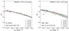 |
Fig. 1. FWHM visibility fitting for two single exposures. The coloured dots with error bars show the visibilities measured at different baselines. The best-fitting results from Eq. (1) are shown as black solid lines; the grey shaded regions show the 1σ fitting uncertainties. The dates and the UTC time are shown in the bottom left corners of each panel. The left panel illustrates a typical exposure, while the right panel shows an example of poor-quality data. |
3. Hot dust size measurements
Interferometric resolution is determined by the baseline length B between telescopes and the observed wavelength λ as λ/2B (Eisenhauer et al. 2023); in the case of the UTs of the VLTI, the resolution reaches ∼2 mas in K band. However, one can measure the size of an object with about ten times better resolution by measuring how the contrast (or visibility) of the interferometric fringes decreases with larger baseline length (GRAVITY Collaboration 2020b). In doing this, the squared visibility (VIS2DATA, hereafter V2) is used instead of the visibility amplitude (VISAMP) in the reduced GRAVITY FT data because the former shows less coherence loss (GRAVITY Collaboration 2020b; Leftley et al. 2021).
We measured the size of the hot dust by fitting the V2 of the FT continuum data to a Gaussian model,
 (1)
(1)
where V0 is the zero baseline visibility, ruv is the baseline length in units of mas−1, and FWHM in mas is the full width at the half maximum of the source emission. Following GRAVITY Collaboration (2020b), we also allowed V0 to be free in the fitting to account for the remaining coherence loss of the calibrated data and/or extended flux that is resolved out by the interferometer. We fitted the visibility data from each individual exposure (with ∼5 min exposure time for the on-axis mode, and 2 min for the off-axis mode), and found the best-fitting zero baseline V0 and FWHM using the scipy function curve_fit. Figure 1 shows two such examples. The clear drops in V2 with increasing baseline lengths indicate that the hot dust continuum is resolved. We only incorporated the three central channels (2.07, 2.17, and 2.27 μm) of the FT data in the fitting because the remaining three channels are more susceptible to the detector background due to the metrology laser at the shorter wavelength and the thermal background at the longer wavelength.
We present the measured FWHM of each target in Table 2. We specifically included only those exposures for which the fitted error is less than one-third of the FWHM value. Subsequently, we calculated the median of these selected exposures to obtain the measured FWHM for each target. To estimate the FWHM uncertainty, GRAVITY Collaboration (2020b) use the RMS scatter of the FWHM from individual exposures and divide it by the square root of the number of nights. In this way, they account for the night-to-night systematic uncertainty, which likely comes from the variation in the AO performance. This method, however, cannot be applied to most of our targets because they were only observed once. Using the AGNs observed in multiple epochs to investigate the night-to-night FWHM variation, we find that it is about 10% of the averaged FWHM of each night. Therefore, we estimated the FWHM uncertainty by summing in quadrature two components: (1) the statistical uncertainty, which is the RMS scatter of FWHM values divided by the square root of the number of exposures; (2) the systematic uncertainty, which is 10% of the median FWHM. Our method provides FWHM uncertainties consistent with those adopted by GRAVITY Collaboration (2020b) for the targets observed on multiple nights.
Angular and physical size measurements.
Next, we converted the measured Gaussian FWHM to a physical continuum radius. Following GRAVITY Collaboration (2020b), we first converted the Gaussian FWHM to a ring radius by dividing by a factor of  . We then corrected for a putative contamination due to the unresolved central source (the accretion disk and/or jet) with a flux fraction of f by scaling up the ring radius by a factor of
  . The flux fraction f differs for each object, and we used a typical constant value f = 20% (Kishimoto et al. 2009) in our conversions into physical radii. A variation in f between different individual sources would introduce a small uncertainty (< 10%) to the derived sizes. The results are reported in Table 2.
At the end of the table, we provide updated measurements for two sources previously published in GRAVITY Collaboration (2020b). The updated FWHM values remain consistent with the previous measurements (0.59 ± 0.08 for PDS 456 and 0.54 ± 0.06 for Mrk 509). The reduction in uncertainties is attributed to the acquisition of additional exposures in 2021. Specifically, the updated sizes are based on approximately 1.5 times the number of exposures used for the previous published measurements.
4. Dust radius-luminosity relation
We measured the size of 12 new targets and updated two previous measurements with GRAVITY in this work. In Table 3 we compile from the literature all other dust size OI measurements in the K band obtained to date. The last four targets were observed by Keck, while all the others were observed by GRAVITY. IRAS 13349+2438 has been observed by both Keck and GRAVITY; the ring size we measured with GRAVITY is consistent with the Keck measurement of 0.92 ± 0.06 pc reported by Kishimoto et al. (2009). We chose to adopt the more recent result measured by GRAVITY for this study. The compiled data set allowed us to study the dust radius-luminosity (R − L) relation. Together with the literature results, we compiled a sample of 25 type 1 AGNs with OI measured host dust structure sizes. For comparison, we also included 29 AGNs with an RM measured continuum size collected in Table 1 of our companion paper, GRAVITY Collaboration (2023). In that paper we collected the latest measurements of the hot dust continuum by OI and RM for z ≲ 0.2 AGNs, and our main focus was to investigate the relation between the BLR and the dust continuum size. Throughout this work, we adopted the continuum size directly converted from the time delay without applying any redshift correction (e.g. Minezaki et al. 2019), because the wavelength dependence of continuum emission size is expected to be less than 10% for our low-z sample (GRAVITY Collaboration 2023).
Literature physical size measurements.
We collected the AGN luminosity from the literature following the method introduced in GRAVITY Collaboration (2020b). Briefly, we collected the AGN 14−195 keV X-ray (L14 − 195 keV), optical (5100 Å,  ), and 12 μm (λLλ(12 μm)) monochromatic luminosities whenever available. The X-ray luminosity comes from the Swift/BAT observations (Baumgartner et al. 2013). We discarded the X-ray luminosities of 3C 273 and PDS 456 due to contamination from jet emission and significant variability, respectively. The optical luminosities are taken from GRAVITY Collaboration (2023), and the λLλ(12 μm) comes from the high-resolution MIR observations by Asmus et al. (2011).
Fundamentally, the dust is heated by the central optical/UV continuum source, and thus the size is expected to depend on the total optical-UV luminosity (Barvainis 1987). However, measuring optical-UV luminosity is challenging due to various factors. We opted to use the bolometric luminosity that can be derived from various methods. As detailed in Appendix A, we calculated Lbol based on 14–195 keV measurements whenever possible, using non-linear corrections. In cases where such measurements are unavailable, we opted for values derived from the optical luminosity (see Table A.1 for details). We included the λLλ(12 μm) to provide additional comparison to quantify the uncertainty of the bolometric luminosities and the R − L relations. The differences in Lbol estimates from different monochromatic luminosities agree to within 0.3 dex, which we adopt as the uncertainty.
We fitted the R − L relations of the bolometric luminosity and various monochromatic luminosities in the form of Eq. (2) using the linmix package, which is a Python version of LINMIX_ERR from Kelly (2007),
 (2)
(2)
where c and m are the regression intercept and slope, respectively; R is the measured dust continuum size in pc; L is the luminosity; and L0 is fixed at the same value for both the OI and RM relations to reduce the degeneracy of the regression coefficients. In LINMIX_ERR, the probability distribution of the independent variable is modelled as a mixture of K Gaussian functions, and we use K = 2 for all of our fittings throughout this work. We use the median values of the c and m coefficients obtained from the likelihood distributions generated by LINMIX_ERR as the best-fit regression coefficients. The uncertainties associated with these coefficients are determined from the 16th and 84th percentiles of their likelihood distributions. We also characterise the intrinsic scatter of the linear regression, σintrin, using the median value from its distribution. The best-fit parameters with uncertainties are listed in Table 4.
Results of linear regression of R − L relations for OI and RM measurements.
We first fit the dust size R as a function of bolometric luminosity. Figure 2 shows the relation of R − Lbol to the continuum sizes measured by the OI and RM, respectively. The best-fit slope for ROI is about 0.45, slightly shallower than, but consistent within ∼1σ of, the expected R ∝ L0.5. The best-fit slope for RRM is entirely consistent with that of ROI. The uncertainty of the slope can be further reduced by expanding the sample with high and low luminosities. The intrinsic scatter for the ROI relation is 0.2 dex, similar to that of the RRM relation. We do not find a significant correlation between the offsets from the fitted dust R − L relation and the Eddington ratio with the OI measurements.
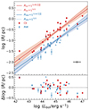 |
Fig. 2. Dust radius as a function of bolometric luminosity (R − Lbol relation). OI measured sizes are shown in red and RM measured sizes are shown in blue. The typical 0.3 dex uncertainty in Lbol is indicated in the right corner. The solid lines show our best-fit results, with the shaded regions showing the 1σ uncertainties of the fittings, while the dotted lines represent the fitting results with the slopes m fixed to 0.5. Our best-fitting R − Lbol relations are consistent with the slope of 0.5 within 1σ. The bottom panel shows the dust radius residuals from the fitted relation with fixed slopes of 0.5. |
Our compilation of the literature measurements cannot guarantee that the continuum size and the AGN luminosities are measured close in time. Kishimoto et al. (2013) showed in NGC 4151 that any change in luminosity will not immediately affect the measured dust sublimation radius, only if the change persists over several years. A potential explanation for this reduced response to AGN variability proposed by Hönig & Kishimoto (2011) is the ‘snowball’ model, in which clouds only gradually sublimate at the inner edge of the torus. In this case the dust size may be relatively constant with time in a typical AGN, and the AGN variability itself may be the dominant source of intrinsic scatter (see more discussion in GRAVITY Collaboration 2023).
We also fit the R − L relations using different monochromatic luminosities (L14 − 195 keV,  , and λLλ(12 μm)) and their corresponding bolometric luminosity following the equations in Appendix A. Using monochromatic luminosities separates spectral energy distribution (SED) effects that potentially influence dust structure size, while converting them to Lbol with appropriate bolometric corrections aligns R − L relations across wavelengths, mitigating differences related to the observed luminosity’s wavelength. The results for all these R − L relations are shown in Fig. 3 and Table 4.
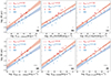 |
Fig. 3. The R − L relations using different monochromatic luminosities and their corresponding bolometric luminosity. The top panels show the relations between the dust size and the monochromatic luminosities at (a) 14−195 keV, (b) optical 5100 Å, and (c) 12 μm. The bottom panels (d)–(f) show the R − L relation of the bolometric luminosity converted from these three monochromatic luminosities. The symbols are the same as in Fig. 2. The slopes of the relations using the RM and OI measurements agree with each other in all the luminosities we investigated. For the OI measurements, all the R − L relationships agree within 1σ with a slope of 0.5, except for the optical luminosity |

As in Fig. 2, we find that the slopes of the OI-measured R − L relations consistently agree with those of the RM-measured relations for each type of luminosity in Fig. 3. For the monochromatic luminosities shown in the top row of Fig. 3, the slopes of the relations vary with wavelength, probably due to the SED change as a function of luminosity. The slopes of the  R − L relation in panel b shows the most significant deviation from the 0.5 power law, which is close to 3σ. This finding is consistent with previous studies from Minezaki et al. (2019) and Sobrino Figaredo et al. (2020). Various explanations have been discussed by these authors to interpret the observed shallower slope, such as anisotropic illumination by the accretion disk, non-trivial composition and geometry of the dust structure, delayed dust sublimation responses, and non-linear correlations between optical and UV luminosities. For detailed discussions and references of these interpretations, we refer to Minezaki et al. (2019) and Sobrino Figaredo et al. (2020).
On the other hand, we find that R − L relations using bolometric luminosities derived from optical luminosities with non-linear bolometric corrections show slopes consistent with the canonical R ∝ L0.5 relation within 1σ (notably panel e in Fig. 3). For the OI measurements, the slopes of the R − L relations fitted using bolometric luminosities are all in line with the canonical value of 0.5. Therefore, we suggest that comparing the slope of the R − L relation observed using monochromatic luminosities (or a simple linear bolometric correction) to the canonical value of 0.5 may be misleading because the relation between monochromatic luminosities and dust heating is sensitive to the SED shape. The adopted non-linear bolometric correction in our approach, which results in steeper slopes than the monochromatic R − L relations, may reflect the systemic dependency of SED shape on luminosities (e.g. Vignali et al. 2003; Netzer 2019; Duras et al. 2020).
Recent RM studies using WISE W1 (3.4 μm) and W2 (4.6 μm) data support our conclusion. Several works (Chen et al. 2023; Mandal et al. 2024) reporting their R − L relation slope shallower than 0.5, either used the  or a V-band luminosity with a constant bolometric correction. In contrast, Lyu et al. (2019) applied a non-linear bolometric correction, which was different from our approach, and reported a slope similar to our result. Similar differences in slopes between
  and Lbol are also evident in the BLR R − L relations (Abuter et al. 2024). For studying the R − L relations, we recommend using the more accurate non-linear correction (e.g. Netzer 2019; Duras et al. 2020) rather than a linear approximation for the bolometric luminosities.
In all the fits of R − L relations we have examined, the intrinsic scatters are predominantly below 0.2 dex. Typically, the intrinsic scatters from monochromatic luminosities are slightly larger than those from bolometric luminosities. This may be due to the larger uncertainty assigned to the bolometric luminosities, while the larger scatter in the monochromatic luminosities likely reflects the specific characteristics of the SEDs of individual sources. Contamination of the NIR continuum from compact jet emission in some sources (Fernández-Ontiveros et al. 2023) could also contribute to the scatter in the R − L relations. Additionally, the intrinsic scatter is influenced by the range of luminosities and the number of data points used for the fitting. For instance, the higher intrinsic scatter from L14 − 195 keV is likely due to the small range of luminosity, because of the lack of high-luminosity objects in this sample. Additionally, a smaller range of luminosity also introduces a larger uncertainty on the fitted slopes. Nevertheless, the relatively small intrinsic scatter from all the relations indicates that the R − L relations are tightly constrained.
5. Constraining the hot dust structure
The R − L relations from the OI and RM measurements have similar slopes. However, there is a general offset between the two relations. As shown in Table 4, the intercepts (m) fitted from the OI data are ∼0.3 − 0.4 dex larger than those from the RM method. This means the hot dust continuum size measured by OI is in general about 2–2.5 times larger than that measured by the RM time lag. This has been attributed to the difference between the flux-weighted radius and response-weighted radius of the innermost hot dust (Koshida et al. 2014). Moreover, Sobrino Figaredo et al. (2020) argue that the large ROI/RRM ratio can be explained by the ‘foreshortening effect’ of a bowl-shaped dust structure (Pozo Nuñez et al. 2014; Oknyansky et al. 2015; Ramolla et al. 2018). In this section we adopt a simple model of hot dust emission to explore how the observed ROI/RRM can be used to constrain the model. Our goal is to obtain qualitative properties of the hot dust structure based on the samples of OI and RM observations, while more quantitative measurements of the hot dust structure of individual sources must be obtained by modelling of the OI and RM data in detail.
We incorporate a simple model, as described in Guise et al. (2022). The hot dust emission comes from a 2D surface which can be flaring above the midplane, as shown in Fig. 4. The model is flexible enough to generate the bowl-shaped structure that was proposed previously (e.g. Kawaguchi & Mori 2010; Goad et al. 2012) and supported by RM observations (e.g. Pozo Nuñez et al. 2014; Oknyansky et al. 2015; Ramolla et al. 2018; Sobrino Figaredo et al. 2020). The model assumes that the dust distribution is optically thick in the vertical direction, so that the IR emission is dominated by the surface of the structure facing the observer. The details of the model are summarised in Appendix B. Briefly, the model consists of a large number of dust clouds, each in thermal equilibrium and radiating as black bodies. The cloud radial distribution is controlled by a power-law index α, while cloud heights above the midplane are controlled by another power-law index β. A higher α means more emission from the outer region, while the curved surface becomes steeper with increasing β. The model is observed at an inclination angle i. Only one side of the dust emission can be observed because the other side, which is behind the midplane, is fully obscured in NIR (see Appendix B for adopted dust temperature and SED). As illustrated by Fig. 4 (assuming i = 0° with the line of sight downwards from the top for simplicity), the bowl-shaped (one-sided) dust emission naturally leads to an RM time lag smaller than the projected size of the hot dust, the ‘foreshortening effect’ (Sobrino Figaredo et al. 2020, and references therein). To account for the observational effect that we measure the size of the hot dust interferometrically, we simulate the V2 of the model assuming a typical size, distance, and baseline lengths of our targets. We measure the ROI of the simulated V2 in the same way as our targets, by fitting a Gaussian model and converting the FWHM to a ring radius (see details in Sect. 3); we do not apply additional correction for the central point source, as the model does not incorporate its flux contribution. Meanwhile the time lag (RRM ≡ cτRM) is calculated as the flux-weighted mean time lag of all the dust clouds. Both the sizes ROI and RRM are in units of the dust sublimation radius rsub. Exploration of the parameter space shows that such a model can easily reproduce ROI/RRM ≈ 2, while other properties of the model match various independent observational constraints.
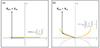 |
Fig. 4. Sketch of the hot dust structure model. The hot dust emission is in yellow. The cloud radial distribution follows a power law with the index α, and the cloud height above the midplane is close to a power-law function controlled by β. Panel a shows the model with β ≈ 0, while panel b shows a model with β > 0. We show the models in an edge-on view with the observer to the positive direction of h to illustrate the ‘foreshortening effect’. In this way model (a) has RRM ≈ ROI, while model (b) has RRM < ROI. |
As shown in Fig. 5, we calculate the ROI/RRM ratio of the model with −0.5 < α < 2.0 and 0 < β < 2.0 viewed with inclinations of 0°, 10°, 20°, and 40°. To guide the eye, we highlight a fiducial model with α = 1.0 and β = 1.0, which corresponds to a conical structure. The corresponding ROI/RRM decreases from around 2.5 to around 1.5 when the inclination increases from 0° to 40°. At fixed inclination, the ratio increases when α and β increase because more emission comes further away from the midplane and the ‘foreshortening effect’ is stronger. When α ≳ 1, the ROI/RRM ratio mainly depends on β because the hot dust emission mainly comes from the outer edge of the model.
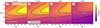 |
Fig. 5. Exploration of the parameter space of the hot dust structure model. The colour maps show the derived ROI/RRM ratio based on different α and β in grids. The four columns present the model with different inclination angles (i from 0° to 40°). The geometric covering factor of the model is labelled on the left. A fiducial model, which can qualitatively explain our observed ROI/RRM ≈ 2, is indicated by the cyan star. |
The model parameters can be further constrained by our other knowledge from observation and theory. Within our preferred parameter space, RRM typically falls within one or two times rsub, consistent with theoretical expectations and previous observations (e.g. Kishimoto et al. 2007; Koshida et al. 2014). The SED of the hot dust emission has also been studied by many observational (e.g. Nenkova et al. 2008a; Mor & Netzer 2012; Lani et al. 2017; Shangguan et al. 2018; Zhuang et al. 2018) and theoretical works (e.g. Fritz et al. 2006; Nenkova et al. 2008b; Hönig & Kishimoto 2010, 2017). The SED of the hot dust emission is affected by α and β because the dust grains further from the heating source have lower temperature. As discussed in Appendix B, the NIR colours of our model are largely consistent with the radiation transfer model (CAT3D; Hönig & Kishimoto 2017) when −0.5 < α < 2.0 and 0.5 < β < 1.5. Moreover, we calculate the geometric covering factor of the bowl-shaped structure based on the maximum h/r of the clouds (h as cloud height and r as radial distance),  . The cf only depends on β because we assume the 2D surface is fully filled for simplicity in Fig. 5. When β increases, the accretion disk is more likely to be obscured by the dust, namely the covering factor cf is higher, because a more solid angle is covered by the dusty structure. Various observations indicate the dust covering factor is typically 0.6−0.8, for example from the fraction of obscured AGNs (Huchra & Burg 1992; Ricci et al. 2017), dust-reprocessed AGN luminosity fraction (Stalevski et al. 2016), and modelling the X-ray spectrum (Zhao et al. 2021). We find that in the model, the geometric covering factor is ∼0.7 when β ≈ 1.0, consistent with the observations.
The ratio ROI/RRM in our sample appears relatively constant across the entire luminosity range; however, intriguing variations might arise depending on other properties of the AGNs. Ricci et al. (2017) found that the dust covering factor of AGNs with a high Eddington ratio (e.g. λEdd ≳ 0.1) is much lower than the low-Eddington ratio AGNs. In the context of our model, this means β decreases significantly when λEdd > 0.1. Since the ROI/RRM is sensitive to β, we expect to find low ROI/RRM for sources with high λEdd. However, the current small sample size does not allow a robust statistical analysis on this. More observations of high-Eddington ratio AGNs will be valuable in exploring this dependence. In addition, the model suggests that there is an inclination dependence of ROI/RRM. It would be also interesting to investigate the relationship between inclination and ROI/RRM by gathering independent estimations of inclination for a statistically significant sample.
In summary, we conducted a heuristic search of the parameter space of a simple hot dust model to find where ROI/RRM is around 2. We find that a bowl-shaped dust emitting structure can explain the observed values with the ratio primarily affected by the inclination angle and β of the model. Moreover, the covering factor of the preferred model is consistent with other independent observations. Our modelling illustrates that combining the OI and RM observations is a powerful way to constrain the structure of the hot dust emission. The geometric distance based on the joint analysis of the OI and RM observations should account for variation of inclination and opening angle of the bowl-shaped structure for individual sources.
6. Summary
-
We present new measurements of the hot dust structure sizes of 14 type 1 AGNs from VLTI/GRAVITY interferometric observation. The typical full width at half maximum (FWHM) is ∼0.7 mas, comparable to previous near-infrared sizes, and 10−20 times smaller than mid-infrared sizes in the literature.
-
We compiled a sample of 25 AGNs at z ≲ 0.2 with hot dust sizes measured by optical/infrared interferometry, covering four orders of magnitude in luminosity, to study the R − L relation. We also compiled a sample of 29 AGNs at comparable redshifts with RM measured continuum sizes for comparison. The analysis shows a tight correlation between the size of the innermost hot dust structure and AGN luminosity, with an intrinsic scatter of less than 0.2 dex, consistent for both OI and RM measured relations.
-
The slopes of the OI and RM R − L relations are consistent with the canonical value of 0.5 (R ∝ L0.5) within 1σ if we adopt more accurately derived bolometric luminosity with a non-linearity correction. Meanwhile, we find the slope of the relation deviates from 0.5 most significantly with the optical luminosity. We emphasise that proper bolometric corrections should be used when the R − L relation is investigated.
-
Converted to physical sizes, our direct measurements from GRAVITY show an offset of a factor of 2 compared to the equivalent relation derived through reverberation mapping. We used a simple model to explore dust structure geometry, and conclude that a bowl-shaped hot dust structure could explain the size ratio in harmony with other physical constraints.
Hereafter we use the term time lag interchangeably with RRM ≡ cτRM for simplicity.
Observations were made using the ESO Telescopes at the La Silla Paranal Observatory, programme IDs 1103.B-0626 and 0109.B-0270.
The time lag of the ith cloud is τi = ri(1 − cos ψi).
Some CAT3D models show a low J − H colour (e.g. at 1.2 < H − K < 1.8) primarily because the accretion disk emission contaminates the colour when the torus emission is very red.
Acknowledgments
Based on observations collected at the European Southern Observatory under ESO programmes 1103.B-0626 and 0109.B-0270. We thank Keiichi Wada for helpful discussions. We also thank the anonymous referee for a constructive report and helpful suggestions. This research has used the NASA/IPAC Extragalactic Database (NED), operated by the California Institute of Technology, under contract with the National Aeronautics and Space Administration. This research has used the SIMBAD database, operated at CDS, Strasbourg, France.
References
- Abuter, R., Allouche, F., Amorim, A., et al. 2024, Nature, 627, 281 [NASA ADS] [CrossRef] [Google Scholar]
- Antonucci, R. R. J., & Miller, J. S. 1985, ApJ, 297, 621 [NASA ADS] [CrossRef] [Google Scholar]
- Asmus, D., Gandhi, P., Smette, A., Hönig, S. F., & Duschl, W. J. 2011, A&A, 536, A36 [NASA ADS] [CrossRef] [EDP Sciences] [Google Scholar]
- Asmus, D., Hönig, S. F., Gandhi, P., Smette, A., & Duschl, W. J. 2014, MNRAS, 439, 1648 [NASA ADS] [CrossRef] [Google Scholar]
- Baldassare, V. F., Reines, A. E., Gallo, E., & Greene, J. E. 2015, ApJ, 809, L14 [NASA ADS] [CrossRef] [Google Scholar]
- Barvainis, R. 1987, ApJ, 320, 537 [Google Scholar]
- Baumgartner, W. H., Tueller, J., Markwardt, C. B., et al. 2013, ApJS, 207, 19 [Google Scholar]
- Burtscher, L., Meisenheimer, K., Tristram, K. R. W., et al. 2013, A&A, 558, A149 [NASA ADS] [CrossRef] [EDP Sciences] [Google Scholar]
- Chen, Y.-J., Liu, J.-R., Zhai, S., et al. 2023, MNRAS, 522, 3439 [NASA ADS] [CrossRef] [Google Scholar]
- Clavel, J., Wamsteker, W., & Glass, I. S. 1989, ApJ, 337, 236 [NASA ADS] [CrossRef] [Google Scholar]
- Duras, F., Bongiorno, A., Ricci, F., et al. 2020, A&A, 636, A73 [NASA ADS] [CrossRef] [EDP Sciences] [Google Scholar]
- Eisenhauer, F., Monnier, J. D., & Pfuhl, O. 2023, ARA&A, 61, 237 [NASA ADS] [CrossRef] [Google Scholar]
- Fernández-Ontiveros, J. A., López-López, X., & Prieto, A. 2023, A&A, 670, A22 [NASA ADS] [CrossRef] [EDP Sciences] [Google Scholar]
- Fritz, J., Franceschini, A., & Hatziminaoglou, E. 2006, MNRAS, 366, 767 [Google Scholar]
- Gámez Rosas, V., Isbell, J. W., Jaffe, W., et al. 2022, Nature, 602, 403 [CrossRef] [Google Scholar]
- Goad, M. R., Korista, K. T., & Ruff, A. J. 2012, MNRAS, 426, 3086 [Google Scholar]
- GRAVITY Collaboration (Abuter, R., et al.) 2017, A&A, 602, A94 [NASA ADS] [CrossRef] [EDP Sciences] [Google Scholar]
- GRAVITY Collaboration (Sturm, E., et al.) 2018, Nature, 563, 657 [Google Scholar]
- GRAVITY Collaboration (Pfuhl, O., et al.) 2020a, A&A, 634, A1 [NASA ADS] [CrossRef] [EDP Sciences] [Google Scholar]
- GRAVITY Collaboration (Dexter, J., et al.) 2020b, A&A, 635, A92 [NASA ADS] [CrossRef] [EDP Sciences] [Google Scholar]
- GRAVITY Collaboration (Amorim, A., et al.) 2021a, A&A, 648, A117 [NASA ADS] [CrossRef] [EDP Sciences] [Google Scholar]
- GRAVITY Collaboration (Amorim, A., et al.) 2021b, A&A, 654, A85 [NASA ADS] [CrossRef] [EDP Sciences] [Google Scholar]
- GRAVITY Collaboration (Abuter, R., et al.) 2022, A&A, 665, A75 [NASA ADS] [CrossRef] [EDP Sciences] [Google Scholar]
- GRAVITY Collaboration (Amorim, A., et al.) 2023, A&A, 669, A14 [NASA ADS] [CrossRef] [EDP Sciences] [Google Scholar]
- GRAVITY Collaboration (Amorim, A., et al.) 2024, A&A, 684, A167 [NASA ADS] [CrossRef] [EDP Sciences] [Google Scholar]
- Guise, E., Hönig, S. F., Gorjian, V., et al. 2022, MNRAS, 516, 4898 [NASA ADS] [CrossRef] [Google Scholar]
- Hönig, S. F. 2019, ApJ, 884, 171 [Google Scholar]
- Hönig, S. F., & Kishimoto, M. 2010, A&A, 523, A27 [NASA ADS] [CrossRef] [EDP Sciences] [Google Scholar]
- Hönig, S. F., & Kishimoto, M. 2011, A&A, 534, A121 [NASA ADS] [CrossRef] [EDP Sciences] [Google Scholar]
- Hönig, S. F., & Kishimoto, M. 2017, ApJ, 838, L20 [Google Scholar]
- Hönig, S. F., Kishimoto, M., Tristram, K. R. W., et al. 2013, ApJ, 771, 87 [Google Scholar]
- Huchra, J., & Burg, R. 1992, ApJ, 393, 90 [NASA ADS] [CrossRef] [Google Scholar]
- Kawaguchi, T., & Mori, M. 2010, ApJ, 724, L183 [Google Scholar]
- Kelly, B. C. 2007, ApJ, 665, 1489 [Google Scholar]
- Kishimoto, M., Hönig, S. F., Beckert, T., & Weigelt, G. 2007, A&A, 476, 713 [NASA ADS] [CrossRef] [EDP Sciences] [Google Scholar]
- Kishimoto, M., Hönig, S. F., Antonucci, R., et al. 2009, A&A, 507, L57 [NASA ADS] [CrossRef] [EDP Sciences] [Google Scholar]
- Kishimoto, M., Hönig, S. F., Antonucci, R., et al. 2011a, A&A, 536, A78 [CrossRef] [EDP Sciences] [Google Scholar]
- Kishimoto, M., Hönig, S. F., Antonucci, R., et al. 2011b, A&A, 527, A121 [CrossRef] [EDP Sciences] [Google Scholar]
- Kishimoto, M., Hönig, S. F., Antonucci, R., et al. 2013, ApJ, 775, L36 [NASA ADS] [CrossRef] [Google Scholar]
- Kishimoto, M., Anderson, M., ten Brummelaar, T., et al. 2022, ApJ, 940, 28 [NASA ADS] [CrossRef] [Google Scholar]
- Koshida, S., Minezaki, T., Yoshii, Y., et al. 2014, ApJ, 788, 159 [Google Scholar]
- Koss, M., Trakhtenbrot, B., Ricci, C., et al. 2017, ApJ, 850, 74 [Google Scholar]
- Lani, C., Netzer, H., & Lutz, D. 2017, MNRAS, 471, 59 [NASA ADS] [CrossRef] [Google Scholar]
- Lapeyrere, V., Kervella, P., Lacour, S., et al. 2014, SPIE Conf. Ser., 9146, 91462D [Google Scholar]
- Leftley, J. H., Tristram, K. R. W., Hönig, S. F., et al. 2018, ApJ, 862, 17 [Google Scholar]
- Leftley, J. H., Tristram, K. R. W., Hönig, S. F., et al. 2021, ApJ, 912, 96 [NASA ADS] [CrossRef] [Google Scholar]
- Leftley, J. H., Petrov, R., Moszczynski, N., et al. 2024, A&A, 686, A204 [NASA ADS] [CrossRef] [EDP Sciences] [Google Scholar]
- López-Gonzaga, N., Burtscher, L., Tristram, K. R. W., Meisenheimer, K., & Schartmann, M. 2016, A&A, 591, A47 [NASA ADS] [CrossRef] [EDP Sciences] [Google Scholar]
- Lyu, J., Rieke, G. H., & Smith, P. S. 2019, ApJ, 886, 33 [NASA ADS] [CrossRef] [Google Scholar]
- Mandal, A. K., Woo, J.-H., Wang, S., et al. 2024, ApJ, 968, 59 [NASA ADS] [CrossRef] [Google Scholar]
- Marconi, A., Risaliti, G., Gilli, R., et al. 2004, MNRAS, 351, 169 [Google Scholar]
- McConnell, N. J., Ma, C.-P., Gebhardt, K., et al. 2011, Nature, 480, 215 [NASA ADS] [CrossRef] [Google Scholar]
- Mehrgan, K., Thomas, J., Saglia, R., et al. 2019, ApJ, 887, 195 [NASA ADS] [CrossRef] [Google Scholar]
- Mezcua, M., & Sánchez, H. D. 2024, MNRAS, 528, 5252 [NASA ADS] [CrossRef] [Google Scholar]
- Minezaki, T., Yoshii, Y., Kobayashi, Y., et al. 2019, ApJ, 886, 150 [NASA ADS] [CrossRef] [Google Scholar]
- Mor, R., & Netzer, H. 2012, MNRAS, 420, 526 [NASA ADS] [CrossRef] [Google Scholar]
- Nenkova, M., Sirocky, M. M., Nikutta, R., Ivezić, Ž., & Elitzur, M. 2008a, ApJ, 685, 160 [Google Scholar]
- Nenkova, M., Sirocky, M. M., Ivezić, Ž., & Elitzur, M. 2008b, ApJ, 685, 147 [Google Scholar]
- Netzer, H. 2015, ARA&A, 53, 365 [Google Scholar]
- Netzer, H. 2019, MNRAS, 488, 5185 [NASA ADS] [CrossRef] [Google Scholar]
- Oknyansky, V. L., Gaskell, C. M., & Shimanovskaya, E. V. 2015, Odessa Astron. Publ., 28, 175 [CrossRef] [Google Scholar]
- Planck Collaboration XIII. 2016, A&A, 594, A13 [NASA ADS] [CrossRef] [EDP Sciences] [Google Scholar]
- Pott, J.-U., Malkan, M. A., Elitzur, M., et al. 2010, ApJ, 715, 736 [NASA ADS] [CrossRef] [Google Scholar]
- Pozo Nuñez, F., Haas, M., Chini, R., et al. 2014, A&A, 561, L8 [NASA ADS] [CrossRef] [EDP Sciences] [Google Scholar]
- Prieto, M. A., Reunanen, J., Tristram, K. R. W., et al. 2010, MNRAS, 402, 724 [Google Scholar]
- Prieto, M. A., Nadolny, J., Fernández-Ontiveros, J. A., & Mezcua, M. 2021, MNRAS, 506, 562 [NASA ADS] [CrossRef] [Google Scholar]
- Ramolla, M., Haas, M., Westhues, C., et al. 2018, A&A, 620, A137 [NASA ADS] [CrossRef] [EDP Sciences] [Google Scholar]
- Reines, A. E. 2022, Nat. Astron., 6, 26 [NASA ADS] [CrossRef] [Google Scholar]
- Ricci, C., Trakhtenbrot, B., Koss, M. J., et al. 2017, Nature, 549, 488 [NASA ADS] [CrossRef] [Google Scholar]
- Shakura, N. I., & Sunyaev, R. A. 1973, A&A, 24, 337 [NASA ADS] [Google Scholar]
- Shangguan, J., Ho, L. C., & Xie, Y. 2018, ApJ, 854, 158 [NASA ADS] [CrossRef] [Google Scholar]
- Sobrino Figaredo, C., Haas, M., Ramolla, M., et al. 2020, AJ, 159, 259 [NASA ADS] [CrossRef] [Google Scholar]
- Stalevski, M., Ricci, C., Ueda, Y., et al. 2016, MNRAS, 458, 2288 [Google Scholar]
- Suganuma, M., Yoshii, Y., Kobayashi, Y., et al. 2006, ApJ, 639, 46 [NASA ADS] [CrossRef] [Google Scholar]
- Swain, M., Vasisht, G., Akeson, R., et al. 2003, ApJ, 596, L163 [NASA ADS] [CrossRef] [Google Scholar]
- Trakhtenbrot, B., Ricci, C., Koss, M. J., et al. 2017, MNRAS, 470, 800 [NASA ADS] [CrossRef] [Google Scholar]
- Urry, C. M., & Padovani, P. 1995, PASP, 107, 803 [NASA ADS] [CrossRef] [Google Scholar]
- Vasudevan, R. V., & Fabian, A. C. 2007, MNRAS, 381, 1235 [NASA ADS] [CrossRef] [Google Scholar]
- Vasudevan, R. V., & Fabian, A. C. 2009, MNRAS, 392, 1124 [CrossRef] [Google Scholar]
- Vignali, C., Brandt, W. N., & Schneider, D. P. 2003, AJ, 125, 433 [Google Scholar]
- Weigelt, G., Hofmann, K. H., Kishimoto, M., et al. 2012, A&A, 541, L9 [NASA ADS] [CrossRef] [EDP Sciences] [Google Scholar]
- Winter, L. M., Mushotzky, R. F., Reynolds, C. S., & Tueller, J. 2009, ApJ, 690, 1322 [NASA ADS] [CrossRef] [Google Scholar]
- Winter, L. M., Veilleux, S., McKernan, B., & Kallman, T. R. 2012, ApJ, 745, 107 [NASA ADS] [CrossRef] [Google Scholar]
- Wright, E. L., Eisenhardt, P. R. M., Mainzer, A. K., et al. 2010, AJ, 140, 1868 [Google Scholar]
- Yang, Q., Shen, Y., Liu, X., et al. 2020, ApJ, 900, 58 [NASA ADS] [CrossRef] [Google Scholar]
- Zhao, X., Marchesi, S., Ajello, M., et al. 2021, A&A, 650, A57 [NASA ADS] [CrossRef] [EDP Sciences] [Google Scholar]
- Zhuang, M.-Y., Ho, L. C., & Shangguan, J. 2018, ApJ, 862, 118 [NASA ADS] [CrossRef] [Google Scholar]
Appendix A: Bolometric luminosity correction
We convert each type of measured luminosity to the bolometric luminosity, using non-linear corrections, following the same method as GRAVITY Collaboration (2020b). We collect the 14-195 keV flux from the 70-month Swift-BAT survey catalogue (Baumgartner et al. 2013). We mainly use L14 − 195 keV to calculate the bolometric luminosity following the relation from Winter et al. (2012), which is derived using bolometric luminosities from optical-to-X-ray SED fitting (Vasudevan & Fabian 2007, 2009),
 (A.1)
(A.1)
We also use monochromatic luminosity at 5100 Å following the relation in Trakhtenbrot et al. (2017),
 (A.2)
(A.2)
This relation was obtained using the bolometric correction for the B band from Marconi et al. (2004) based on luminosity-dependent SED templates, and additionally assuming a constant UV-to-optical spectral slope for the conversion from B-band correction to 5100 Å.
For the MIR flux, we first convert 12 μm flux f12 μm to 2 − 10 keV flux f2 − 10 keV following Asmus et al. (2011),
 (A.3)
(A.3)
then L14 − 195 keV is calculated from 2 − 10 keV luminosity using the relation from Winter et al. (2009),
 (A.4)
(A.4)
Both of the relations are established empirically. Finally the MIR-based bolometric luminosity Lbol, 12 μm is obtained using Eq. A.1.
We list the results of the bolometric luminosities calculated from the above methods in Table A.1. We compare the three different bolometric luminosities in Fig. A.1. We find that the differences are within 0.3 dex, and we use this value as the uncertainty of bolometric luminosities. The variability effect is partially captured within this uncertainty since the luminosities at different bands are collected at different times.
Properties of the AGNs used in this work.
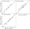 |
Fig. A.1. Comparisons of Lbol corrections from different measurements. The solid dots highlight the sources with OI measured sizes. The dashed lines show the one-to-one relation. The median and standard deviation of y − x are shown in the top-left corner in each panel. |
The bolometric luminosities adopted for studying the R–Lbol relation in this work are listed in column (10) of Table A.1. We prioritise L14 − 195 keV-based bolometric luminosity; when it is unavailable,  -based calculation is used. This preference is due to the L14 − 195 keV-based correction being established with bolometric luminosities reliably determined from SED fitting, whereas additional SED model assumptions were required for the
  -based calculations, potentially leading to extra uncertainties. The λLλ(12 μm)-based bolometric calculation incorporated two empirical relations in addition to the one between Lbol and 14–195 keV luminosity, making it potentially less reliable; therefore, we use it only for comparative evaluations. For AGNs common with with those studied by Prieto et al. (2010), the bolometric luminosities we adopted are consistent with those derived from nuclear SEDs by those authors.
Appendix B: The torus model
Following Guise et al. (2022), we build a torus model to simulate the hot dust emission and time lag in K band. Our primary goal is to investigate whether the observed ROI/RRM ≈ 2 can be explained by a simple model. The model has been discussed comprehensively in Guise et al. (2022). We briefly summarise its key points and clarify our treatments that are different from Guise et al. (2022).
The torus model consists of a large number of dust clouds randomly generated to form a 2D surface. The radial distribution of the clouds follows a power-law probability density function (PDF),
 (B.1)
(B.1)
where r is radial distance of cloud from the center, rsub is the sublimation radius of the dust, and power-law index, α, is a primary free parameter of the model. The underlying radial density of clouds thus follows a power-law with an index of α − 1; a value of α = 1 means a flat density profile at any radius, while a higher α means more clouds distribute to larger distances. We adopted the maximum radius of the clouds to be 20 times that of rsub. However, ROI/RRM is not sensitive to the maximum radius because both ROI and RRM increase with the maximum radius. The height of the clouds above the midplane, h, follows a power-law function,
![Mathematical equation: $$ \begin{aligned} h = r_{\rm sub} \left[\left(\frac{r}{r_{\rm sub}}\right)^\beta -1\right], \end{aligned} $$](/articles/aa/full_html/2024/10/aa50746-24/aa50746-24-eq55.gif) (B.2)
(B.2)
where the power-law index β is another primary parameter of this model. The model is close to a flat disk when β is close to 0, and is close to parabolic when β = 2. Although the dust torus may have a more complicated 3D structure (Hönig 2019), the K-band emission is expected to be emitted from the hottest dust close to the surface of the torus facing the radiation from the accretion disk. Considering the effect of illumination, we include the emission weight of the clouds,
 (B.3)
(B.3)
where ψ is the angle between observer’s line of sight and cloud’s line of sight to the center from the origin (the radiation source). Each dust cloud is assumed to have black body emission in a equilibrium state according to the absorbed emission from the central radiation source, so the dust temperature is,
 (B.4)
(B.4)
where r is the radius of the dust cloud, Tsub is the sublimation temperature, and γ is the dust IR opacity power-law index which is around 1–2 for interstellar dust. We adopt γ = 1.6 for typical astronomical dust following Barvainis (1987), while we find that our conclusions are not sensitive to the adopted γ. We choose to use Tsub = 1900 K, instead of 1500 K adopted by Barvainis (1987), because recent observations found increasing evidence of a higher sublimation temperature due to the graphite dust grains (Mor & Netzer 2012; Hönig & Kishimoto 2017). Our model ROI/RRM is not very sensitive to the Tsub, but as discussed later, we find our model provides consistent JHK colour when adopting Tsub = 1900 K.
In order to calculate the ROI, we first simulate the observed visibility of the dust torus model with the realistic baseline lengths of GRAVITY and apply the same fitting method as described in Sect. 3. The torus time lag is calculated as the flux-weighted mean time lag of each cloud3. In this work, we use the model in a heuristic manner to investigate whether there is a parameter range that can explain our observed ROI/RRM. We explored mainly the parameter space defined in Guise et al. (2022). We found that α ≈ 1.0 is preferred to obtain ROI/RRM ≈ 2, much larger than the parameter range defined in Guise et al. (2022) (−5.5 < α < −0.5). The α controls the radial distribution of the dust clouds so it influences the SED of the model. Our preferred α ranges are not necessary the same as theirs since we are focusing on K-band observations, while Guise et al. (2022) are working in longer wavelengths. We compare the JHK colours predicted by our model to the CAT3D model (Hönig & Kishimoto 2017), one of the state-of-the-art torus models considering different temperatures of the graphite and silicon dust and the polar wind structure. We focus on the JHK colours because, unlike CAT3D, our model only consider the hottest dust in the torus surface. As shown in Fig. B.1, the J − H and H − K colours of our simple model matches those of the CAT3D model4 in the parameter ranges that we adopt in this work, in particular, −0.5 < α < 2. We also find that our model will become much redder than the CAT3D model if we use Tsub = 1500 K, likely because that the CAT3D model includes the graphite dust with the sublimation temperature at 1900 K. The comparison with JHK colours suggest that the dust distribution of our model is reasonable. The conclusion is not sensitive to the choice of the radiative transfer model as long as the Tsub is assumed consistently. We prefer to compare our model colours with the radiative transfer models over the real observation because the observed AGN SED are contaminated by the host galaxy which is usually bright in NIR. In summary, we confirm that our adopted parameter ranges align with the theoretically expected colour of the torus.
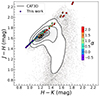 |
Fig. B.1. J − H and H − Ks relation of our torus model (colour-coded) comparing that of the CAT3D-wind model (in black). We calculated our torus model with −0.5 < α < 2.0, 0.5 < β < 1.5, and i < 40°. We include the CAT3D-wind model SEDs with i < 45° for comparison. |
All Tables
All Figures
|
Fig. 1. FWHM visibility fitting for two single exposures. The coloured dots with error bars show the visibilities measured at different baselines. The best-fitting results from Eq. (1) are shown as black solid lines; the grey shaded regions show the 1σ fitting uncertainties. The dates and the UTC time are shown in the bottom left corners of each panel. The left panel illustrates a typical exposure, while the right panel shows an example of poor-quality data. |
| In the text | |
|
Fig. 2. Dust radius as a function of bolometric luminosity (R − Lbol relation). OI measured sizes are shown in red and RM measured sizes are shown in blue. The typical 0.3 dex uncertainty in Lbol is indicated in the right corner. The solid lines show our best-fit results, with the shaded regions showing the 1σ uncertainties of the fittings, while the dotted lines represent the fitting results with the slopes m fixed to 0.5. Our best-fitting R − Lbol relations are consistent with the slope of 0.5 within 1σ. The bottom panel shows the dust radius residuals from the fitted relation with fixed slopes of 0.5. |
| In the text | |
|
Fig. 3. The R − L relations using different monochromatic luminosities and their corresponding bolometric luminosity. The top panels show the relations between the dust size and the monochromatic luminosities at (a) 14−195 keV, (b) optical 5100 Å, and (c) 12 μm. The bottom panels (d)–(f) show the R − L relation of the bolometric luminosity converted from these three monochromatic luminosities. The symbols are the same as in Fig. 2. The slopes of the relations using the RM and OI measurements agree with each other in all the luminosities we investigated. For the OI measurements, all the R − L relationships agree within 1σ with a slope of 0.5, except for the optical luminosity |
| In the text | |
|
Fig. 4. Sketch of the hot dust structure model. The hot dust emission is in yellow. The cloud radial distribution follows a power law with the index α, and the cloud height above the midplane is close to a power-law function controlled by β. Panel a shows the model with β ≈ 0, while panel b shows a model with β > 0. We show the models in an edge-on view with the observer to the positive direction of h to illustrate the ‘foreshortening effect’. In this way model (a) has RRM ≈ ROI, while model (b) has RRM < ROI. |
| In the text | |
|
Fig. 5. Exploration of the parameter space of the hot dust structure model. The colour maps show the derived ROI/RRM ratio based on different α and β in grids. The four columns present the model with different inclination angles (i from 0° to 40°). The geometric covering factor of the model is labelled on the left. A fiducial model, which can qualitatively explain our observed ROI/RRM ≈ 2, is indicated by the cyan star. |
| In the text | |
|
Fig. A.1. Comparisons of Lbol corrections from different measurements. The solid dots highlight the sources with OI measured sizes. The dashed lines show the one-to-one relation. The median and standard deviation of y − x are shown in the top-left corner in each panel. |
| In the text | |
|
Fig. B.1. J − H and H − Ks relation of our torus model (colour-coded) comparing that of the CAT3D-wind model (in black). We calculated our torus model with −0.5 < α < 2.0, 0.5 < β < 1.5, and i < 40°. We include the CAT3D-wind model SEDs with i < 45° for comparison. |
| In the text | |
Current usage metrics show cumulative count of Article Views (full-text article views including HTML views, PDF and ePub downloads, according to the available data) and Abstracts Views on Vision4Press platform.
Data correspond to usage on the plateform after 2015. The current usage metrics is available 48-96 hours after online publication and is updated daily on week days.
Initial download of the metrics may take a while.