| Issue |
A&A
Volume 689, September 2024
|
|
|---|---|---|
| Article Number | A27 | |
| Number of page(s) | 7 | |
| Section | Extragalactic astronomy | |
| DOI | https://doi.org/10.1051/0004-6361/202450413 | |
| Published online | 30 August 2024 | |
The size-luminosity relation of the AGN torus determined from the comparison between optical and mid-infrared variability
1
Department of Astronomy and Atmospheric Sciences, Kyungpook National University, Daegu 41566, Korea
2
Kavli Institute for Astronomy and Astrophysics, Peking University, Beijing 100871, China
3
Department of Astronomy, School of Physics, Peking University, Beijing 100871, China
Received:
17
April
2024
Accepted:
10
June
2024
Abstract
We investigate the optical variability of low-redshift (0.15 < z ≤ 0.4) active galactic nuclei using multi-epoch data from the Zwicky Transient Facility. We find that a damped random walk model describes well the ensemble structure function in the g band. Consistent with previous studies, more luminous active galactic nuclei tend to have a steeper structure function at a timescale less than the break timescale and a smaller variability amplitude. By comparing the structure functions in the optical with the mid-infrared obtained from the Wide-field Infrared Survey Explorer, we derive the size of the dusty torus using a toy model for the geometry of the torus. The size of the torus positively correlates with the luminosity of the active nucleus, following a relation that agrees well with previous studies based on reverberation mapping. This result demonstrates that the structure function method can be used as a powerful and highly efficient tool to examine the size of the torus.
Key words: quasars: general / galaxies: Seyfert
Corresponding author; This email address is being protected from spambots. You need JavaScript enabled to view it. .
© The Authors 2024
 Open Access article, published by EDP Sciences, under the terms of the Creative Commons Attribution License (https://creativecommons.org/licenses/by/4.0), which permits unrestricted use, distribution, and reproduction in any medium, provided the original work is properly cited.
This article is published in open access under the Subscribe to Open model. This email address is being protected from spambots. You need JavaScript enabled to view it. to support open access publication.
1. Introduction
The ultraviolet-optical continuum from unobscured active galactic nuclei (AGNs) originates in the thermal emission from the accretion disk. It is known to vary over a wide range of timescales, from days to years (e.g., Ulrich et al. 1997). While the physical origin of the ultraviolet-optical variability is still under debate, recent observational studies argue that it could be attributed to thermal instability, in which the variability timescale scales with the orbital timescale or black hole mass (e.g., Kelly et al. 2009; Sun et al. 2020; Burke et al. 2021; Arévalo et al. 2023; Tang et al. 2023). The intrinsic variability is often modeled with a damped random walk, in which the power spectral density (PSD) decreases with increasing frequency as a power law (i.e., PSD ∝ ν−2) at high frequency above the break frequency (ν ≫ νbreak) and flattens at low frequency (ν ≤ νbreak; Kelly et al. 2011). At the same time, AGNs exhibit a strong mid-infrared (MIR) continuum emitted from dust heated in a donut-shaped torus around the supermassive black hole and accretion disk. The MIR emission also varies in response to the ultraviolet-optical continuum (e.g., Kozlowski et al. 2016; Son et al. 2022). The characteristics of MIR variability are mostly determined by the combination of the intrinsic variability in the accretion disk and the geometry of the dusty torus, indicating that it can be used to probe the structure of the torus (e.g., Li & Shen 2023; Son et al. 2023a).
Variability has been widely used to investigate the physical properties of the central structures in AGNs. In particular, the reverberation mapping (RM; Blandford & McKee 1982) technique allows us to derive the size of central components robustly. This method has been applied primarily to estimate the size of the broad-line region (BLR) by estimating the time lag between the ultraviolet-optical continuum from the accretion disk and the fluxes of various broad emission lines emitted from the dense material in the BLR, which is ionized by the high-energy photons from the accretion disk (e.g., Peterson et al. 2004; Bentz et al. 2009; Du et al. 2015; Shen et al. 2023; Woo et al. 2024). Recently, the size of the accretion disk has been evaluated for a handful of nearby AGNs (e.g., Mrk 142, NGC 4593, and NGC 5548) using X-ray and ultraviolet-optical continuum RM (e.g., Fausnaugh et al. 2016; Cackett et al. 2018, 2020).
The time lag between the ultraviolet-optical continuum and IR continuum has been used to constrain the size of the torus (Suganuma et al. 2006; Koshida et al. 2014 for the K band, and Lyu et al. 2019; Yang et al. 2020; Mandal et al. 2024 for 3.4 − 4.6 μm), with the aid of multi-epoch near-infrared (NIR) data from ground-based telescopes and MIR light curves from the Wide-field Infrared Survey Explorer (WISE; Wright et al. 2010). These studies have revealed that the size of the torus is positively correlated with the AGN luminosity. Prior or parallel to these RM works, observational studies with the MIR interferometry also demonstrated similar results (e.g., Kishimoto et al. 2011; Burtscher et al. 2013; GRAVITY Collaboration 2020). This size-luminosity relation is also found in the BLR RM studies. In addition, the size of the torus increases with increasing rest-frame wavelength, indicating that the inner part of the torus is hotter than the outer part, consistent with the torus model (e.g., Lyu et al. 2019). However, because the RM method requires intensive observations of high cadence and long duration for individual objects, it can only be applied to a limited number of targets.
Alternatively, Li & Shen (2023) demonstrate that the comparison between the ultraviolet-optical and MIR variability can provide statistically valuable constraints on the size of the dusty torus. Although this method cannot be applied to an individual object, it permits the investigation of the average geometry of the torus in a sample of AGNs sharing similar properties. Moreover, unlike the RM method, it does not require simultaneous, multi-epoch, multiwavelength data with a regular cadence for a single target. Therefore, this method is suitable for existing time-series surveys.
Active galactic nuclei variability is known to follow a damped random walk, which is well described by a broken power-law PSD (e.g., Kelly et al. 2009; Kozlowski et al. 2010; but see Mushotzky et al. 2011; Kasliwal et al. 2015). However, characterization of the PSD requires multi-epoch data with regular and dense sampling, as a consequence of which the PSD of ultraviolet-optical light curves has been estimated robustly for relatively small samples (Smith et al. 2018). An alternative and effective strategy to study the characteristics of AGN variability utilizes the structure function (SF), which is defined as the root mean square of the magnitudes at a given time difference, Δt. The SF is relatively free from bias due to sparse and irregular sampling, and it reasonably approximates a damped random walk (e.g., Hughes et al. 1992; MacLeod et al. 2010; Kozlowski 2016). On the other hand, unless the multi-epoch data are well sampled with a dense cadence and sufficiently long baseline, it is hard to fully constrain the SF of a single object (Kozlowski 2016). To overcome this limitation, one can utilize an ensemble SF computed by averaging the SFs from multiple objects at a given timescale. In particular, ensemble SFs have been widely used to examine how AGN variability depends on the physical properties of AGNs (e.g., Trevese et al. 1994; Vanden Berk et al. 2004; Son et al. 2023a).
Li & Shen (2023) adopted a simple toy model for the torus, one solely determined by the torus geometry without considering radiative transfer, in order to compute the torus transfer function. From a direct comparison between the ensemble SFs of the optical and MIR variability, in conjunction with the torus transfer function, Li & Shen (2023) investigated the size of the torus for a sample of relatively luminous [log (Lbol/erg s−1)≥45.3] and distant (0.5 ≤ z ≤ 1.2) quasars selected from the multi-epoch optical photometric data from Stripe 82 of the Sloan Digital Sky Survey (SDSS; Abazajian et al. 2009; Annis et al. 2014) and MIR photometry from WISE. In good agreement with previous studies conducted with the RM method, this experiment showed that the size of the torus positively correlates with the AGN luminosity (Li & Shen 2023).
In this study, we apply the methodology of Li & Shen (2023) to examine whether the size-luminosity relation applies to quasars of lower redshift (0.15 < z ≤ 0.4) and lower luminosity [44.4 ≤ log (Lbol/erg s−1)≤45.9]. In particular, the narrow range of redshift is essential to minimize the dependence of the torus size on rest-frame wavelength. Section 2 describes the sample selection and data. Section 3 presents the detailed method of constructing the ensemble SFs. The comparison between the optical and MIR SFs is shown in Section 4, and the size-luminosity relation from our method is given in Section 5. Section 5 summarizes the overall results. We adopt the cosmological parameters H0 = 100 h = 67.4 km s−1 Mpc−1, Ωm = 0.315, and ΩΛ = 0.685 (Planck Collaboration VI 2020).
2. Sample and data
For a direct comparison between the optical and MIR SFs, we adopted the same sample of type 1 AGNs from Son et al. (2023a), for which the MIR SF was computed using the light curves from WISE. The parent sample was initially drawn from the Data Release 14 quasar catalog of the SDSS (Pâris et al. 2018). To minimize the effect of cosmic evolution on the dust properties and photometric uncertainties introduced by the extended features of the host galaxy, Son et al. (2023a) imposed a redshift cut of 0.15 < z ≤ 0.4. To secure NIR and MIR data, Son et al. (2023a) selected sources with 2MASS (Skrutskie et al. 2006) and WISE counterparts with a matching radius of 2″, to arrive at a sample of 4295 type 1 AGNs. Son et al. (2023a) demonstrated that the NIR data are crucial to properly constrain the flux contribution from the host galaxy (Son et al. 2022, 2023a).
To obtain the optical light curves in the g band, we crossmatched the initial sample from Son et al. (2023a) with the Zwicky Transient Facility (ZTF) Data Release 19 using a matching radius of 2″ (Bellm et al. 2019). We find that all the sources have counterparts in ZTF. The average baseline and cadence of the optical light curves are ∼1785 days and ∼21.7 days, respectively. To remove any suspicious measurements, we only used the photometric data with flag = 0, a separation angle of  , and a limiting g-band magnitude of < 20.2. These criteria were carefully determined from visual inspection of the light curves to discard outliers in the photometric measurements (e.g., timescale of spikes and dips less than a few days). To reconstruct the SF robustly, we chose sources that have ZTF photometric data from at least 20 epochs. Finally, to only consider variable sources, we adopted the criterion Pvar ≥ 0.95, which is the probability that the target is genuinely variable, calculated from χ2 statistics (Sánchez-Sáez et al. 2018; Son et al. 2023a). Pvar was estimated after the host galaxy contribution was subtracted. It is worth noting that the selection criterion of 0.95 is suitable for selecting weakly or moderately variable sources: ∼87% of the entire sample meets this criterion. Without this selection, SFs with large photometric uncertainties can introduce systematic bias in the ensemble estimation. Radio-loud AGNs may exhibit enhanced variability due to the relativistic jet. We computed the radio-loudness of the sample using the 1.4 GHz luminosity (L1.4 GHz) from the FIRST survey and i-band luminosity (Li), in which a K-correction was applied by assuming a spectral index of −0.5 (Richards et al. 2006; Kimball & Ivezić 2008). The radio-loud AGNs were classified with a criterion of R > 1, where R was defined as L1.4 GHz/Li (Baloković et al. 2012). These radio-loud sources were finally excluded from further analysis. This reduced the final sample to 3578 objects.
The bolometric luminosity was estimated from the continuum luminosity at 5100 Å with a bolometric correction of Lbol = 9.26 L5100 derived from the mean spectral energy distribution of type 1 quasars (Richards et al. 2006), where L5100 was computed from spectral fitting of the SDSS spectra (Rakshit et al. 2020). We adopted the bolometric luminosities based on L5100 instead of alternatives such as those derived from the strength of [O III] λ5007 (Son et al. 2023a), which is sensitive to the covering factor of the narrow-line region, the ionization parameter, and the shape of the ionizing continuum (e.g., Heckman et al. 2004; Shen et al. 2011; Kong & Ho 2018; Netzer 2019). While the bolometric correction is known to be sensitive to the AGN luminosity, its uncertainty is typically smaller than 0.1 dex in the range of the AGN luminosity in our sample (e.g., Hopkins et al. 2007; Netzer 2019). The final sample has a median z = 0.296, Mg = −22.03 mag, log (MBH/M⊙) = 8.19, log (Lbol/erg s−1) = 45.2, and log (Lbol/LEdd) = − 1.05. We followed Son et al. (2023a) and calculated the black hole mass, MBH, using the virial method and spectral measurements of Rakshit et al. (2020).
3. Structure function
We quantified the optical variability with the SF, defined as the mean difference of the magnitude in the light curve as a function of the time lag (Δt):
 (1)
(1)
where NΔt, pair denotes the number of pairs associated with Δt, m is the magnitude, and σe represents the uncertainty of the magnitude in each epoch. In general, AGN light curves can be described by a damped random walk in which the SF is proportional to the time lag at Δt < τ (SF ∝ Δt1) and flattens at Δt ≥ τ (SF ∝ Δt0), where τ is the break timescale. This can be expressed more generally as
![Mathematical equation: $$ \begin{aligned} \mathrm{SF} = \left[\mathrm{SF^2_{\infty }} (1-e^{(-\Delta t/\tau )^\gamma })\right]^{0.5}, \end{aligned} $$](/articles/aa/full_html/2024/09/aa50413-24/aa50413-24-eq3.gif) (2)
(2)
where SF∞ is the SF at Δt ≫ τ and γ is the power-law slope for Δt < τ (i.e., SF ∝ Δtγ). The damped random walk model can be expressed with γ = 1. The uncertainty of the SF for an individual target was computed from the square root of the standard deviation of  at a given Δt (see Equation 1).
3.1. Host galaxy contribution
Although the ZTF survey provides photometry in both g and r, we used the g-band data because it is less contaminated by the flux from the host galaxy. Nevertheless, we estimated the flux contribution from the host in the g band by fitting the spectral energy distribution that spans from the optical to the MIR, constructed from measurements from SDSS, 2MASS, and WISE. Following the detailed fitting method described in Son et al. (2023b), we adopted three spectral energy distribution templates for AGNs (hot dust-deficient, warm dust-deficient, and normal AGNs) from Lyu et al. (2017) and seven templates for the host galaxy from Polletta et al. (2007), which comprise an old (7 Gyr) stellar population and galaxies of Hubble type E, S0, Sa, Sb, Sc, and Sd. The derived host flux from the individual target was subtracted from the original light curve. The average host fraction in the g band is only ∼0.12, which has a minor effect on the SF measurements.
3.2. Photometric uncertainty
The SF is known to be highly sensitive to photometric error, and its effect is severe when estimating the slope on short timescales (e.g., Kozlowski 2016). To check whether the photometric uncertainties (σo) provided by the ZTF survey are reliable, we used the ZTF light curves of non-variable sources drawn from the inactive galaxies from the Max Planck Institute for Astrophysics and the Johns Hopkins University (MPA–JHU) catalog (Brinchmann et al. 2004). From the SF calculated from the individual object without removing the contribution from the photometric noise,  . We applied the same criteria as the science data for the AGN sample to select reliable photometric measurements. If the original photometric error (σo) is estimated robustly, the SFs are expected to equal
  . Instead, we find
  (Figure 1), which indicates that the photometric noise is underestimated. To account for this, we adopted a final photometric error of σe = 0.9σo.
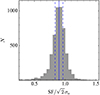 |
Fig. 1. Distribution of SFs divided by |

3.3. Ensemble structure function
As in the work of Son et al. (2023a) on the MIR SF of AGNs, this study utilizes the ensemble SF, which is the average value of the SFs for a number of objects at a given Δt. The ensemble SFs are useful to examine statistically the characteristics of the variability as a function of various AGN properties, using light curves with sparse and irregular cadences (e.g., Vanden Berk et al. 2004; Bauer et al. 2009).
The reliability of the SF also depends on the cadence and baseline of the light curves. To test this, we made 10 000 mock light curves that were modeled with a damped random walk, for which the sampling of the mock light curve was randomly taken from the real observations of ZTF for our sample. To mimic the ZTF light curves of our sample, we generated the input light curves assuming that SF∞ = 0.38, τ = 350 days, γ = 1, and that the photometric uncertainty is 0.068 mag. We then computed the ensemble SF using two different estimators: the square root of the mean SF2 and the mean of SF. Our simulations show that the ensemble SF is slightly overestimated at Δt < 15 days, as is also seen in the observed data (Figure 2). If the photometric error is larger than the intrinsic SF, the mean observed SF2 occasionally could be smaller than zero, which should be excluded in the calculation of the ensemble SF. This can boost the SF at small Δt, where the intrinsic SF is smaller than the photometric noise. Therefore, this study uses the ensemble SF at Δt ≥ 15 days. Son et al. (2023a) demonstrated, and the simulation in Figure 2 confirms, that the square root of the mean SF2 is a better tracer of the real ensemble SF than the mean of SF. We also computed the ensemble SFs in the same manner. Finally, the uncertainties in the ensemble SF were estimated from bootstrap resampling of the SFs of the individual target within the uncertainty of the individual SF. We performed 1000 realizations of resampling, and the final uncertainty was estimated from half of the difference between the 16th and 84th percentiles.
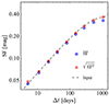 |
Fig. 2. Ensemble SFs derived from the mock light curves. The 10 000 light curves were generated to mimic the real multi-epoch data from ZTF. The dashed line denotes the input SF. The red squares and blue circles represent the square root of the mean SF2 and the mean of SF, respectively. |
4. Results
4.1. The g-band structure function
We first estimated the ensemble g-band SF of the entire sample (Figure 3; Table 1). The break timescale, τ, is known to be correlated with black hole mass and AGN luminosity (e.g., Kelly et al. 2009; MacLeod et al. 2010; Burke et al. 2021; Tang et al. 2023). However, the relatively short time baseline of the ZTF survey makes it difficult to estimate τ robustly with this dataset. Although we only use Equation (2) to investigate the qualitative form of the SF, without attaching any specific physical meaning to it at this stage, we nevertheless derived a power-law slope of γ = 0.99 ± 0.05, which agrees well with the prediction from the damp random walk model.
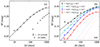 |
Fig. 3. (a) Ensemble SFs of the entire sample. Open circles represent the SF for the optical data from ZTF, with the solid line denoting their fit to a broken power law. Filled circles give the SF for the MIR data from Son et al. (2023a). (b) Ensemble SFs of the subsamples binned by the continuum luminosity at 5100 Å. Open symbols and solid lines are the SFs and fitting results for the optical data, while the dashed lines show the corresponding SFs for the MIR data. |
Structure function parameters.
Dividing the sample into four luminosity bins reveals that γ is proportional to luminosity, such that more luminous AGNs exhibit a steeper SF over short timescales than fainter sources. The parameter SF∞ is inversely correlated with the AGN luminosity (Table 1). These findings are consistent with the trends reported in previous studies, not only in terms of MIR variability (Son et al. 2023a) but also optical variability (e.g., Vanden Berk et al. 2004; MacLeod et al. 2010; Tang et al. 2023).
4.2. Fitting with the torus model
The MIR light curves can be expressed as the combination of the intrinsic light curve from the accretion disk and the transfer function of the dusty torus,
 (3)
(3)
where LMIR is the MIR light curve, Ψ(τ) is the transfer function of the torus, and Lopt is the ultraviolet-optical continuum light curve. We adopted the torus model of Li & Shen (2023), for which the transfer function of the torus is determined solely by its geometry, which is described by an inner radius (Rin), a half-opening angle (θ) representing the angle between the equatorial plane and the edge of the torus, an outer to inner radius ratio (Y), and an inclination angle (i). A total of 50 000 clouds were generated following a power-law density distribution (p = −1 for ρ ∝ rp) in a radial direction.
We additionally considered a damping factor (d ≡ SF∞, MIR/SF∞, opt), which is the fraction of the variability amplitude between the optical and the MIR. This term is necessary because the variability amplitude of the MIR data is significantly smaller than that of the optical data (i.e., d < 1; Neugebauer et al. 1989; Kozlowski et al. 2010, 2016). We adopted the Python codes from Li & Shen (2023)1 but modified them by adding the damping factor in order to fit the MIR SFs more robustly. The grid of predicted MIR SFs, generated with the input optical light curve and the torus transfer function computed from the torus model, spans the following range of parameters: −1.85 ≤ log(Rin/pc)≤ − 0.1, 0° < i < 45°, 1.3 ≤ Y ≤ 1.5, σ = 30°, and 0.45 ≤ d ≤ 0.8. While the range of Rin was determined based on the results from the previous NIR and MIR RM projects (e.g., Koshida et al. 2014; Lyu et al. 2019), that of Y was inferred from the morphology of hot dust derived from the NIR interferometric observations (e.g., Kishimoto et al. 2009). We used the grid of modeled SFs to fit the observed MIR SFs from Son et al. (2023a). Because the optical SFs only securely cover Δt < 1000 days, we used the same range of Δt to fit the MIR SFs.
The transfer function – and therefore the shape – of the MIR SFs was mostly determined by the combination of Rin, Y, and a power-law index for the density distribution (p; e.g., Almeyda et al. 2020). To keep the consistency of the method with Li & Shen (2023), we first adopted the small Y and a fixed p. The best fit for the entire sample yields Rin = 0.18 ± 0.01 pc (Figure 4a), which is in good agreement with the torus sizes derived from the RM method and interferometric observations of nearby Seyferts, [42.5 ≲ log (Lbol/erg s−1)≲46.5] at ∼2.2 μm (e.g., Kishimoto et al. 2011; Koshida et al. 2014).
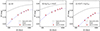 |
Fig. 4. Fitting results of the MIR SFs for (a) the entire sample, (b) the least luminous sources, and (c) the most luminous sources. The solid line is the optical SF estimated from the ZTF survey. Red points represent the MIR SF from the WISE survey, with the dashed blue line denoting the best fit. |
5. The size-luminosity relation of the torus
We applied the fit for the ensemble SFs to the subsamples divided by AGN luminosity. Fitting the faintest (Figure 4b) and brightest (Figure 4c) AGNs clearly shows that, as was expected, Rin is correlated with the AGN luminosity (Table 2). We compared our results with those obtained from RM studies, which investigated the size-luminosity relation of the torus using the time lag between the optical light curves obtained from ground-based telescopes and MIR light curves derived from WISE (e.g., Koshida et al. 2014; Lyu et al. 2019; Yang et al. 2020). The MIR light curves of low-redshift (z < 0.5) Palomar-Green (PG; Schmidt & Green 1983) quasars studied by Lyu et al. (2019) are comparable to those of our sample. They demonstrated a strong correlation between the size of the torus determined in the W1 band and the AGN luminosity, in the form  . While the intrinsic scatter in the size-luminosity relation was not reported in Lyu et al. (2019), using more distant quasars at 0.3 < z < 2 Yang et al. (2020) found a size-luminosity relation similar to that of Lyu et al. (2019); this is illustrated by the gray area in Figure 5, which has an intrinsic scatter of 0.17 dex.
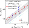 |
Fig. 5. Size-luminosity relation of the torus of type 1 AGNs. Gray squares denote the inner radius of the torus derived from fitting the MIR SFs with the toy model of the torus. Red circles represent the effective size of the torus estimated from the best-fit transfer function, with the solid red line giving their ordinary distance regression fit to the size-luminosity relation. The uncertainties of Rin are the same as those of Reff. The dashed gray line shows the size-luminosity relation of low-redshift (z < 0.5) PG quasars estimated using the RM method (Lyu et al. 2019). The shaded gray area represents the 1σ scatter (∼0.17 dex) estimated from a sample of relatively high-redshift (0.3 < z < 2) AGNs (Yang et al. 2020). The dotted blue line is the relation of intermediate-redshift (0.5 ≤ z ≤ 1.2) quasars in Stripe 82, based on a direct comparison between the optical SFs and MIR (W1) SFs, similar to this study. The dash-dotted cyan line denotes the relation of the local Seyferts in the K band inferred from the RM method. Blue stars represent the size of the torus estimated from the K-band interferometry measurements (GRAVITY Collaboration 2020). |
Radius of the Torus.
For a direct comparison with previous RM studies, we computed the effective radius (Reff) of the torus determined from the best-fit transfer function. This is equivalent to the effective time delay (τeff) directly measured from the RM method, which is expressed as
 (4)
(4)
The effective time delay depends on the inner radius and the geometry of the torus (e.g., the inclination angle and the ratio of the outer and inner radius). Figure 5 shows that the size-luminosity relation from our study is in good agreement with previous studies within the intrinsic scatter. An ordinary distance regression for our measurements yields
 (5)
(5)
This result demonstrates that the ensemble SF can be as effective as the RM method in statistically estimating the size of the torus. Interestingly, the zero point of the size-luminosity relation from this study is slightly larger than that from Li & Shen (2023). The offset in the torus size ranges from 0.1 to 0.2 dex at log (L5100/erg s−1) = 44.5 − 46. This may be attributed to the dependence of the torus size on the rest-frame wavelength (e.g., Lyu et al. 2019). The rest-frame wavelength (λrest ≈ 1.4 − 2.8 μm) of the MIR data in the sample of Li & Shen (2023) is significantly shorter than that of our sample (λrest ≈ 2.5 − 2.8 μm). The shorter wavelengths likely probe the inner regions of the torus. In support of this interpretation, we note that the K-band time lag from Koshida et al. (2014) (λrest ≈ 2 μm) is marginally shorter than that inferred from the W1-based studies. Interestingly, our estimation agrees well with the results from the K-band interferometry measurements (GRAVITY Collaboration 2020). As our results depend on the adopted model for the torus geometry, the discrepancy in the size-luminosity relation among the different studies may originate from the methodology.
The studies with the MIR interferometry showed that the MIR emitting region (8.5 − 13 μm) is more extended than the NIR emitting region (e.g., Kishimoto et al. 2011). To account for this effect, we examined the dependence of Reff on the outer-to-inner radius ratio (Y) and the radial density distribution (p). The SF fits with a model from 1.5 ≤ Y ≤ 10 and −0.5 ≤ p ≤ −1.0 yield worse results compared to the best-fits with a smaller Y (1.3 ≤ Y ≤ 1.5) and a fixed p = −1. In addition, the inferred Reff becomes remarkably smaller than that from the best-fit results with the smaller Y by up to ∼0.5 dex. This result is not physically meaningful as the inner radius is substantially smaller than the sublimation radius. It reveals that the hot dust emitting the MIR continuum at 2.5−2.8 μm is likely to locate the innermost region of the torus and may not be extended along the radius, which is consistent with previous studies (e.g., Kishimoto et al. 2009, 2011).
6. Conclusions
We derived the optical ensemble SF of the low-redshift and moderately luminous AGNs selected from SDSS using the g-band multi-epoch data obtained from the ZTF survey. We find that a broken power law, similar to the damped random walk, can describe the ensemble SF well. However, more luminous AGNs tend to have steeper slopes in the ensemble SF over short timescales than less luminous AGNs, which may be due to the geometric effect of the accretion disk. Consistent with previous studies, the variability amplitude is also anticorrelated with the AGN luminosity.
Using the toy model of the torus geometry from Li & Shen (2023), we made a comparison between the optical and MIR SFs to estimate the effective size of the torus. As with RM experiments, we find that the effective size of the torus positively correlates with AGN luminosity. The slope of the size-luminosity relation agrees well with that of previous studies, although the zero point of the relation is marginally higher than that derived from the analysis of K-band data for local AGNs and W1-band data for high-redshift AGNs, which implies that the size of the torus increases with increasing rest-frame wavelength. These results demonstrate that a comparison between the optical and MIR SFs for a large sample can be a powerful tool to estimate the size of the torus.
https://github.com/bwv1194/geometric-torus-variability
Acknowledgments
We thank the anonymous referee for the constructive comments that substantially improved the manuscript. This work was supported by the National Key R&D Program of China (2022YFF0503401), the National Science Foundation of China (11991052, 12233001), the China Manned Space Project (CMS-CSST-2021-A04, CMS-CSST-2021-A06), and the National Research Foundation of Korea (NRF), through grants funded by the Korean government (MSIT) (Nos. 2022R1A4A3031306, 2023R1A2C1006261, and RS-2024-00347548).
References
- Abazajian, K. N., Adelman-McCarthy, J. K., Agüeros, M. A., et al. 2009, ApJS, 182, 543 [Google Scholar]
- Almeyda, T., Robinson, A., Richmond, M., Nikutta, R., & McDonough, B. 2020, ApJ, 891, 26 [CrossRef] [Google Scholar]
- Annis, J., Soares-Santos, M., Strauss, M. A., et al. 2014, ApJ, 794, 120 [Google Scholar]
- Arévalo, P., Lira, P., Sánchez-Sáez, P., et al. 2023, MNRAS, 526, 6078 [CrossRef] [Google Scholar]
- Baloković, M., Smolčić, V., Ivezić, Ž., et al. 2012, ApJ, 759, 30 [CrossRef] [Google Scholar]
- Bauer, A., Baltay, C., Coppi, P., et al. 2009, ApJ, 696, 1241 [NASA ADS] [CrossRef] [Google Scholar]
- Bellm, E. C., Kulkarni, S. R., Graham, M. J., et al. 2019, PASP, 131, 018002 [Google Scholar]
- Bentz, M. C., Walsh, J. L., Barth, A. J., et al. 2009, ApJ, 705, 199 [NASA ADS] [CrossRef] [Google Scholar]
- Blandford, R. D., & McKee, C. F. 1982, ApJ, 255, 419 [Google Scholar]
- Brinchmann, J., Charlot, S., White, S. D. M., et al. 2004, MNRAS, 351, 1151 [Google Scholar]
- Burke, C. J., Shen, Y., Blaes, O., et al. 2021, Science, 373, 789 [NASA ADS] [CrossRef] [Google Scholar]
- Burtscher, L., Meisenheimer, K., Tristram, K. R. W., et al. 2013, A&A, 558, A149 [NASA ADS] [CrossRef] [EDP Sciences] [Google Scholar]
- Cackett, E. M., Chiang, C.-Y., McHardy, I., et al. 2018, ApJ, 857, 53 [NASA ADS] [CrossRef] [Google Scholar]
- Cackett, E. M., Gelbord, J., Li, Y.-R., et al. 2020, ApJ, 896, 1 [NASA ADS] [CrossRef] [Google Scholar]
- Du, P., Hu, C., Lu, K.-X., et al. 2015, ApJ, 806, 22 [NASA ADS] [CrossRef] [Google Scholar]
- Fausnaugh, M. M., Denney, K. D., Barth, A. J., et al. 2016, ApJ, 821, 56 [Google Scholar]
- GRAVITY Collaboration (Dexter, J., et al.) 2020, A&A, 635, A92 [NASA ADS] [CrossRef] [EDP Sciences] [Google Scholar]
- Heckman, T. M., Kauffmann, G., Brinchmann, J., et al. 2004, ApJ, 613, 109 [Google Scholar]
- Hopkins, P. F., Richards, G. T., & Hernquist, L. 2007, ApJ, 654, 731 [Google Scholar]
- Hughes, P. A., Aller, H. D., & Aller, M. F. 1992, ApJ, 396, 469 [NASA ADS] [CrossRef] [Google Scholar]
- Kasliwal, V. P., Vogeley, M. S., & Richards, G. T. 2015, MNRAS, 451, 4328 [CrossRef] [Google Scholar]
- Kelly, B. C., Bechtold, J., & Siemiginowska, A. 2009, ApJ, 698, 895 [Google Scholar]
- Kelly, B. C., Sobolewska, M., & Siemiginowska, A. 2011, ApJ, 730, 52 [NASA ADS] [CrossRef] [Google Scholar]
- Kimball, A. E., & Ivezić, Ž. 2008, AJ, 136, 684 [Google Scholar]
- Kishimoto, M., Hönig, S. F., Antonucci, R., et al. 2009, A&A, 507, L57 [NASA ADS] [CrossRef] [EDP Sciences] [Google Scholar]
- Kishimoto, M., Hönig, S. F., Antonucci, R., et al. 2011, A&A, 536, A78 [CrossRef] [EDP Sciences] [Google Scholar]
- Kong, M., & Ho, L. C. 2018, ApJ, 859, 116 [NASA ADS] [CrossRef] [Google Scholar]
- Koshida, S., Minezaki, T., Yoshii, Y., et al. 2014, ApJ, 788, 159 [Google Scholar]
- Kozlowski, S. 2016, ApJ, 826, 118 [CrossRef] [Google Scholar]
- Kozlowski, S., Kochanek, C. S., Stern, D., et al. 2010, ApJ, 716, 530 [CrossRef] [Google Scholar]
- Kozlowski, S., Kochanek, C. S., Ashby, M. L. N., et al. 2016, ApJ, 817, 119 [CrossRef] [Google Scholar]
- Li, J., & Shen, Y. 2023, ApJ, 950, 122 [NASA ADS] [CrossRef] [Google Scholar]
- Lyu, J., Rieke, G. H., & Shi, Y. 2017, ApJ, 835, 257 [NASA ADS] [CrossRef] [Google Scholar]
- Lyu, J., Rieke, G. H., & Smith, P. S. 2019, ApJ, 886, 33 [NASA ADS] [CrossRef] [Google Scholar]
- MacLeod, C. L., Ivezić, Ž., Kochanek, C. S., et al. 2010, ApJ, 721, 1014 [Google Scholar]
- Mandal, A. K., Woo, J. H., Wang, S., et al. 2024, ApJ, 968, 59 [NASA ADS] [CrossRef] [Google Scholar]
- Mushotzky, R. F., Edelson, R., Baumgartner, W., & Gandhi, P. 2011, ApJ, 743, L12 [NASA ADS] [CrossRef] [Google Scholar]
- Netzer, H. 2019, MNRAS, 488, 5185 [NASA ADS] [CrossRef] [Google Scholar]
- Neugebauer, G., Soifer, B. T., Matthews, K., & Elias, J. H. 1989, AJ, 97, 957 [NASA ADS] [CrossRef] [Google Scholar]
- Pâris, I., Petitjean, P., Aubourg, É., et al. 2018, A&A, 613, A51 [Google Scholar]
- Peterson, B. M., Ferrarese, L., Gilbert, K. M., et al. 2004, ApJ, 613, 682 [Google Scholar]
- Planck Collaboration VI. 2020, A&A, 641, A6 [NASA ADS] [CrossRef] [EDP Sciences] [Google Scholar]
- Polletta, M., Tajer, M., Maraschi, L., et al. 2007, ApJ, 663, 81 [NASA ADS] [CrossRef] [Google Scholar]
- Rakshit, S., Stalin, C. S., & Kotilainen, J. 2020, ApJS, 249, 17 [Google Scholar]
- Richards, G. T., Lacy, M., Storrie-Lombardi, L. J., et al. 2006, ApJS, 166, 470 [Google Scholar]
- Sánchez-Sáez, P., Lira, P., Mejía-Restrepo, J., et al. 2018, ApJ, 864, 87 [CrossRef] [Google Scholar]
- Schmidt, M., & Green, R. F. 1983, ApJ, 269, 352 [NASA ADS] [CrossRef] [Google Scholar]
- Shen, Y., Richards, G. T., Strauss, M. A., et al. 2011, ApJS, 194, 45 [Google Scholar]
- Shen, Y., Grier, C. J., Horne, K., et al. 2023, ArXiv e-prints [arXiv:2305.01014] [Google Scholar]
- Skrutskie, M. F., Cutri, R. M., Stiening, R., et al. 2006, AJ, 131, 1163 [NASA ADS] [CrossRef] [Google Scholar]
- Smith, K. L., Mushotzky, R. F., Boyd, P. T., et al. 2018, ApJ, 857, 141 [NASA ADS] [CrossRef] [Google Scholar]
- Son, S., Kim, M., & Ho, L. C. 2022, ApJ, 927, 107 [NASA ADS] [CrossRef] [Google Scholar]
- Son, S., Kim, M., & Ho, L. C. 2023a, ApJ, 958, 135 [CrossRef] [Google Scholar]
- Son, S., Kim, M., & Ho, L. C. 2023b, ApJ, 953, 175 [NASA ADS] [CrossRef] [Google Scholar]
- Suganuma, M., Yoshii, Y., Kobayashi, Y., et al. 2006, ApJ, 639, 46 [NASA ADS] [CrossRef] [Google Scholar]
- Sun, M., Xue, Y., Brandt, W. N., et al. 2020, ApJ, 891, 178 [CrossRef] [Google Scholar]
- Tang, J.-J., Wolf, C., & Tonry, J. 2023, Nat. Astron., 7, 473 [Google Scholar]
- Trevese, D., Kron, R. G., Majewski, S. R., Bershady, M. A., & Koo, D. C. 1994, ApJ, 433, 494 [NASA ADS] [CrossRef] [Google Scholar]
- Ulrich, M.-H., Maraschi, L., & Urry, C. M. 1997, ARA&A, 35, 445 [NASA ADS] [CrossRef] [Google Scholar]
- Vanden Berk, D. E., Wilhite, B. C., Kron, R. G., et al. 2004, ApJ, 601, 692 [Google Scholar]
- Woo, J.-H., Wang, S., Rakshit, S., et al. 2024, ApJ, 962, 67 [NASA ADS] [CrossRef] [Google Scholar]
- Wright, E. L., Eisenhardt, P. R. M., Mainzer, A. K., et al. 2010, AJ, 140, 1868 [Google Scholar]
- Yang, Q., Shen, Y., Liu, X., et al. 2020, ApJ, 900, 58 [NASA ADS] [CrossRef] [Google Scholar]
All Tables
All Figures
|
Fig. 1. Distribution of SFs divided by |
| In the text | |
|
Fig. 2. Ensemble SFs derived from the mock light curves. The 10 000 light curves were generated to mimic the real multi-epoch data from ZTF. The dashed line denotes the input SF. The red squares and blue circles represent the square root of the mean SF2 and the mean of SF, respectively. |
| In the text | |
|
Fig. 3. (a) Ensemble SFs of the entire sample. Open circles represent the SF for the optical data from ZTF, with the solid line denoting their fit to a broken power law. Filled circles give the SF for the MIR data from Son et al. (2023a). (b) Ensemble SFs of the subsamples binned by the continuum luminosity at 5100 Å. Open symbols and solid lines are the SFs and fitting results for the optical data, while the dashed lines show the corresponding SFs for the MIR data. |
| In the text | |
|
Fig. 4. Fitting results of the MIR SFs for (a) the entire sample, (b) the least luminous sources, and (c) the most luminous sources. The solid line is the optical SF estimated from the ZTF survey. Red points represent the MIR SF from the WISE survey, with the dashed blue line denoting the best fit. |
| In the text | |
|
Fig. 5. Size-luminosity relation of the torus of type 1 AGNs. Gray squares denote the inner radius of the torus derived from fitting the MIR SFs with the toy model of the torus. Red circles represent the effective size of the torus estimated from the best-fit transfer function, with the solid red line giving their ordinary distance regression fit to the size-luminosity relation. The uncertainties of Rin are the same as those of Reff. The dashed gray line shows the size-luminosity relation of low-redshift (z < 0.5) PG quasars estimated using the RM method (Lyu et al. 2019). The shaded gray area represents the 1σ scatter (∼0.17 dex) estimated from a sample of relatively high-redshift (0.3 < z < 2) AGNs (Yang et al. 2020). The dotted blue line is the relation of intermediate-redshift (0.5 ≤ z ≤ 1.2) quasars in Stripe 82, based on a direct comparison between the optical SFs and MIR (W1) SFs, similar to this study. The dash-dotted cyan line denotes the relation of the local Seyferts in the K band inferred from the RM method. Blue stars represent the size of the torus estimated from the K-band interferometry measurements (GRAVITY Collaboration 2020). |
| In the text | |
Current usage metrics show cumulative count of Article Views (full-text article views including HTML views, PDF and ePub downloads, according to the available data) and Abstracts Views on Vision4Press platform.
Data correspond to usage on the plateform after 2015. The current usage metrics is available 48-96 hours after online publication and is updated daily on week days.
Initial download of the metrics may take a while.