| Issue |
A&A
Volume 690, October 2024
|
|
|---|---|---|
| Article Number | A99 | |
| Number of page(s) | 18 | |
| Section | Stellar atmospheres | |
| DOI | https://doi.org/10.1051/0004-6361/202450737 | |
| Published online | 04 October 2024 | |
Episodic mass loss in the very luminous red supergiant [W60] B90 in the Large Magellanic Cloud
1
IAASARS, National Observatory of Athens,
Metaxa & Vas. Pavlou St.,
15236
Penteli, Athens,
Greece
2
Department of Physics, National and Kapodistrian University of Athens, Panepistimiopolis,
Zografos
15784,
Greece
3
Cerro Tololo Inter-American Observatory/NSF NOIRLab,
Casilla 603,
La Serena,
Chile
4
Las Campanas Observatory, Carnegie Observatories, Colina El Pino,
Casilla 601,
La Serena,
Chile
5
Astronomical Observatory, University of Warsaw,
Al. Ujazdowskie 4,
00-478
Warsaw,
Poland
★ Corresponding author; This email address is being protected from spambots. You need JavaScript enabled to view it.
Received:
16
May
2024
Accepted:
7
August
2024
Abstract
Context. Despite mounting evidence that extreme red supergiants (RSGs) undergo episodic mass-loss events, their role in RSG evolution remains uncertain. Critical questions remain unanswered, such as whether or not these events can strip the star, and their timescale and frequency.
Aims. This study delves into [W60] B90, one of the most luminous and extreme RSGs in the Large Magellanic Cloud (LMC), with our aim being to search for evidence of episodic mass loss. Our discovery of a bar-like nebular structure at 1 pc, which is reminiscent of the bar around Betelgeuse, raised the question of whether [W60] B90 also has a bow shock, motivating the present study.
Methods. We collected and analyzed proper motion data from Gaia, as well as new multi-epoch spectroscopic and imaging data, and archival time-series photometry in the optical and mid-infrared (MIR). We used MARCS models to derive the physical properties of the star from the spectra.
Results. We find [W60] B90 to be a walkaway star, with a supersonic peculiar velocity in the direction of the bar. We detect shocked emission between the bar and the star, based on the [S II]/Hα > 0.4 criterion, providing strong evidence for a bow shock. The 30 yr optical light curve reveals semi-regular variability, showing three similar dimming events with ΔV ~ 1 mag, a recurrence of ~12 yr, and a rise time of 400 days. We find the MIR light curve to vary by 0.51 mag and 0.37 mag in the WISE1 and WISE2 bands, respectively, and by 0.42 mag and 0.25 mag during the last dimming event. During this event, optical spectroscopy reveals spectral variability (M3 I to M4 I), a correlation between the Teff and the brightness, increased extinction, and, after the minimum, spectral features incompatible with the models. We also find a difference of >300 K between the Teff measured from the TiO bands in the optical and the atomic lines from our J-band spectroscopy.
Conclusions. [W60] B90 is a more massive analog of Betelgeuse in the LMC and therefore the first single extragalactic RSG with a suspected bow shock. Its high luminosity of log(L/L⊙) = 5.32 dex, mass-loss rate, and MIR variability compared to other RSGs in the LMC indicate that it is in an unstable evolutionary state, undergoing episodes of mass loss. Investigating other luminous and extreme RSGs in low-metallicity environments using both archival photometry and spectroscopy is crucial to understanding the mechanism driving episodic mass loss in extreme RSGs in light of the Humphreys-Davidson limit and the “RSG problem”.
Key words: stars: atmospheres / stars: late-type / stars: massive / stars: mass-loss / stars: individual: [W60] B90 / supergiants
© The Authors 2024
 Open Access article, published by EDP Sciences, under the terms of the Creative Commons Attribution License (https://creativecommons.org/licenses/by/4.0), which permits unrestricted use, distribution, and reproduction in any medium, provided the original work is properly cited.
This article is published in open access under the Subscribe to Open model. This email address is being protected from spambots. You need JavaScript enabled to view it. to support open access publication.
1 Introduction
Red supergiants (RSGs) are evolved massive stars with initial masses of 8–25 M⊙ (Ekström et al. 2012; Levesque 2017). During their evolution, RSGs increase their luminosity and therefore manifest larger radii and cooler temperatures, before ending their life by exploding as a supernova (SN) or collapsing directly into a black hole (Smartt 2015; Sukhbold et al. 2016; Adams et al. 2017; Laplace et al. 2020). RSGs are more prone to exhibiting spectral-type variability as they become more luminous and cooler as a consequence of a more unstable state (e.g., Levesque et al. 2007; Dorda & Patrick 2021). Despite the fact that the RSG phase represents only 10% of the lifetime of these stars, most stellar mass loss takes place during this phase of the stellar evolution. Empirical relations have revealed a robust correlation between luminosity and mass loss within the RSG phase (e.g., de Jager et al. 1988; van Loon et al. 2005; Beasor et al. 2020; Humphreys et al. 2020; Yang et al. 2023; Antoniadis et al. 2024). Evidence of episodic mass ejections has been found around luminous RSGs (e.g., NML Cyg, VY CMa, Betelgeuse, RW Cep; Richards et al. 1996; Humphreys et al. 2005, 2007; Decin et al. 2006; Dupree et al. 2022; Anugu et al. 2023). These ejections are associated with gaseous outflows related to surface activity (Humphreys & Jones 2022), which impact the photometric variability in terms of dimming events (e.g., Guinan et al. 2019; Humphreys et al. 2021; Anugu et al. 2023). Especially remarkable was the “Great Dimming” of Betelgeuse when the star unexpectedly decreased its brightness by one magnitude. A multiwavelength follow-up found this phenomenon to be the result of a mass-ejection event that formed dust and obscured the star (Dupree et al. 2020; Montargès et al. 2021; Drevon et al. 2024). Montargès et al. (2021) determined the ejected mass to be between 3 and 120% of the annual mass lost by Betelgeuse, demonstrating that the significance of episodic mass loss is uncertain by two orders of magnitude. Humphreys & Jones (2022) revealed that the episodic outflows of Betelgeuse contribute significantly to its overall mass-loss history. On the other hand, in more extreme RSGs, such as VY CMa, the episodic ejections alone explain the high average mass-loss rate measured for the star.
Despite being one of the brightest stars in the sky, Betelgeuse exhibits many properties that remain unexplained (see e.g., Wheeler & Chatzopoulos 2023). The bow shock and bar structure in the vicinity of the star are particularly unusual (Noriega-Crespo et al. 1997a). The origin of the bar is uncertain: some arguments support the relation to Betelgeuse (Mackey et al. 2012) while others advocate for an interstellar origin (Decin et al. 2012; Meyer et al. 2021). On the contrary, the physics behind the bow shock is well understood, as it is produced when a star moves supersonically and the stellar wind interacts with the interstellar medium (ISM), creating an arc-like shape. Although they are commonly seen in OB runaways (Noriega-Crespo et al. 1997b), only two other cases of Galactic single RSGs are known: μ Cep and IRC-10414 (Cox et al. 2012; Gvaramadze et al. 2014). Their detection is useful for constraining the properties of the local ISM and the stellar wind (Hollis et al. 1992; Kaper et al. 1997). Because of the lack of a sophisticated grid of RSG models that include the wind, deriving the mass-loss rate, ![Mathematical equation: $\[\dot{M}\]$](/articles/aa/full_html/2024/10/aa50737-24/aa50737-24-eq1.png) , directly from optical spectroscopy is still impossible. Instead, the
, directly from optical spectroscopy is still impossible. Instead, the ![Mathematical equation: $\[\dot{M}\]$](/articles/aa/full_html/2024/10/aa50737-24/aa50737-24-eq2.png) of RSGs is commonly derived from the mid-infrared (MIR) excess of the spectral energy distribution (SED) (e.g., Riebel et al. 2012; Yang et al. 2023; Antoniadis et al. 2024). However, this methodology depends on general assumptions such as the gas-to-dust ratio, dust grain size, and the mechanism of the wind, which introduce large uncertainties in the results. Therefore, the bow shock in RSGs provides a unique and independent scheme to estimate the
of RSGs is commonly derived from the mid-infrared (MIR) excess of the spectral energy distribution (SED) (e.g., Riebel et al. 2012; Yang et al. 2023; Antoniadis et al. 2024). However, this methodology depends on general assumptions such as the gas-to-dust ratio, dust grain size, and the mechanism of the wind, which introduce large uncertainties in the results. Therefore, the bow shock in RSGs provides a unique and independent scheme to estimate the ![Mathematical equation: $\[\dot{M}\]$](/articles/aa/full_html/2024/10/aa50737-24/aa50737-24-eq3.png) and compare it with that obtained using other methods.
and compare it with that obtained using other methods.
[W60] B90 is one of the most luminous RSGs in the Large Magellanic Cloud (LMC). It was reported by de Wit et al. (2023), within the ASSESS project (Bonanos et al. 2024, Episodic mAss loSS in Evolved maSsive Stars), to have extreme parameters similar to those of WOH G64 (Levesque et al. 2009). Our discovery of a bar-like structure, similar to the bar of Betelgeuse, at 1 pc from the star in an archival Hubble Space Telescope (HST) image, immediately raised the question of whether [W60] B90 could be the first extragalactic RSG with a bow shock. Moreover, its high luminosity close to the observed upper limit of RSGs in the LMC (log(L/L⊙) = 5.50 dex; Davies et al. 2018) and its high mass-loss rate within the LMC (![Mathematical equation: $\[\dot{M}\]$](/articles/aa/full_html/2024/10/aa50737-24/aa50737-24-eq4.png) = 5.07 × 10⁻⁶ M⊙ yr−1, Antoniadis et al. 2024) indicate that this RSG is in an evolved evolutionary state and is undergoing considerable mass loss.
= 5.07 × 10⁻⁶ M⊙ yr−1, Antoniadis et al. 2024) indicate that this RSG is in an evolved evolutionary state and is undergoing considerable mass loss.
In this paper, we present a detailed analysis of [W60] B90. We collected archival photometry to study the long-term photometric variability and we performed a multi-epoch spectroscopic campaign both to study its current spectral variability and search for evidence of shocked material in the circumstellar environment. In Sect. 2, we describe the observations obtained and the archival data used. In Sect. 3, we investigate the membership of [W60] B90 to the LMC and its relation to the bar. We analyze the spectroscopic data for the circumstellar nebular emission and examine its shocked origin. In Sect. 4, we analyze the light curve, the variability in the optical and the MIR, and present the results derived from our optical and near-infrared (NIR) spectroscopic observations. We discuss the results and evolutionary status of the star in Sect. 5, and summarize our conclusions in Sect. 6.
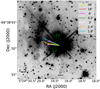 |
Fig. 1 HST F675W image of [W60] B90 showing the PM analysis for PLMC = 0.7. The arrows represent the peculiar velocity direction of [W60] B90 for each cone to compute the local PM of the LMC. The length of the arrows is scaled with the peculiar velocity. The green dotted lines show the 1σ PM error from Gaia DR3 on the 4.5′ cone size. |
2 Observations and data reduction
We discovered a nebular bar structure located at 4″ from [W60] B90 on an HST image available in the Hubble Legacy Archive1 (see Fig. 1). The observations were obtained on 2007 July 27 UT05:34:16 under the program ID 10583, with an exposure time of 1000s and the F675W filter. Below, we describe the archival photometry collected and our spectroscopic observations of [W60] B90.
2.1 Photometric catalogs
We assembled the light curve of [W60] B90 by compiling archival photometry2 spanning ~30 yr from the following surveys: ATLAS forced photometry (Tonry et al. 2018; Heinze et al. 2018; Shingles et al. 2021), ASAS (Pojmanski 1997), ASAS-SN (Shappee et al. 2014; Kochanek et al. 2017), Gaia DR3 (Gaia Collaboration 2016, 2023), the MACHO project (Alcock et al. 1997), NEOWISE (Mainzer et al. 2011), OGLE (Udalski et al. 1997, 2008, 2015), the Spitzer SAGE and SAGE-var projects (Meixner et al. 2006; Riebel et al. 2015), and WISE (Wright et al. 2010; Cutri et al. 2021). We applied the following criteria to each survey to select the most reliable data:
ATLAS: We used forced photometry on reduced images to obtain the light curve from the server. We used data points with flag err = 0, chi/N < 100, and an error below 0.1 mag.
ASAS: We used the photometry based on the smallest aperture (2 px) to avoid contamination from other sources due to the small pixel scale of the instrument (16″px−1). We used the mean data, (i.e., B flag-category) to obtain a cleaner light curve.
ASAS-SN: We retrieved the data from Sky Patrol, selecting the image subtraction with the reference flux added option as it uses co-added data, considerably decreasing the photometry error. We rejected epoch photometry with errors above 0.1 mag, and removed the bm camera data in the g-band, due to a systematic offset in the flux with respect to the other cameras.
Table 1Log of the long-slit observations with the 6.5 m Baade telescope.
MACHO: We only used the VKC-band as the star saturates in the RKC-band. The MACHO calibration uses the VKC − RKC color (see Eq. (1) and (2) in Alcock et al. 1999), and therefore we computed the VKC -band considering the approximation VKC ≈ VM,t + a0 + 2.5 log(ET), where a0 is the zero-point coefficient and ET is the exposure time. We applied a 3σ clipping to discard outliers with small errors.
NEOWISE: [W60] B90 has been observed since the mission started in 2014 during 20 epochs, each lasting over one week. We binned all the photometric measurements within an epoch by taking the median value and the uncertainty of the median. We discarded data with qual_frame = 0 and chi2 > 20. However, NEOWISE photometry differs from ALLWISE for targets brighter than W1 < 8 mag and W2 < 7 mag. Hence, we applied an offset according to Fig. 6 in Mainzer et al. (2014) to correct the magnitudes.
OGLE: We used I-band data from the OGLE-III shallow survey (Ulaczyk et al. 2013), and V-band data from the OGLE-II, OGLE-III, and OGLE-IV databases. Unfortunately, the star is saturated in the images of the main I-band monitoring of the LMC by OGLE, conducted continuously over the last 27 years.
Spitzer: we collected the epoch photometry from the SAGE and SAGE-var projects.
2.2 Optical spectroscopy
We performed spectroscopic observations with the Magellan Echellette (MagE) spectrograph (Marshall et al. 2008) placed on the 6.5 m Baade telescope at Las Campanas Observatory, Chile. We used the 0.7″ × 10″ long-slit, providing a wavelength coverage of 3500–9500Å, a spectral resolution of R ~ 5000, and a spatial resolution of 0.3″ px−1 with binning 1 × 1. Table 1 shows the coordinates of the slit center, UT date of the observations, the instrument, the exposure time, the position angle (PA) of the slits, and the slit width. The slits labeled Epoch1-Epoch4 were centered on the RSG, while slits Neb1-Neb6 were placed around the star to search for shocked material. We used the MagE pipeline (Kelson et al. 2000; Kelson 2003) for the bias and flat correction. We continued the reduction based on the ECHELLE package of IRAF3, as we detected small artifacts in later steps of the MagE pipeline that could compromise the nebular emission. Finally, we used a flux standard to calibrate in flux the spectra with the IRAF routines STANDARD and SENSFUNC.
We divided each slit into small sections to investigate the spatial distribution of the nebular emission. We extracted several apertures of 3 px (0.9″ or ~0.25 pc for the distance of the LMC) in areas of the slits without contamination from background sources (see Table B.1). We consider the 3 px aperture optimal as it minimizes the stellar contamination, achieves a better spatial resolution of the analysis of the circumstellar material (CSM), provides an adequate signal-to-noise ratio (S/N), and avoids a large impact from artifacts. The slits labeled Epoch1 and Neb1-3 did not have acquisition images. We obtained their position and orientation using the header parameters instead.
2.3 Near-infrared spectroscopy
We observed [W60] B90 with the Folded-port InfraRed Echellete (FIRE) instrument placed on the 6.5 m Baade telescope at Las Campanas Observatory, Chile, on 2021 January 30 (Table 1). Using the 0.6″ slit and the binning 1 × 1, we covered the range 0.84–2.4 μm with a spectral resolution of R ~ 6000 and pixel scale of 0.15″ px−1. We obtained four exposures of 15 seconds with the high-gain mode following an ABBA pattern. We reduced the data with the official FIRE pipeline developed in IDL4, including the telluric correction and the flux calibration of the spectra.
2.4 Spitzer spectroscopy
[W60] B90 was observed spectroscopically by Spitzer with the Infrared Spectrograph (IRS) (Houck et al. 2004) inside the programs ID1094 (AORKEY: 6076928) and ID40061 (AORKEY: 22272512). Four modules were used (Short-Low, Short-High, Long-Low, and Long-High) covering the spectral region from 5.2 to 38 μm and providing low (R ~ 60–130) and high (R ~ 600) resolution for the short and long configurations. However, we used only the Short-Low of Program ID1094 from Level 2 of the Post Basic Calibrated Data (PBCD) because an unidentified nearby source contaminated the longer wavelengths. This source is comparable in brightness to [W60] B90 only in MIPS1 (24 μm) images. The data from program ID40061 were discarded, as the star was not properly centered on the slit on the short-low exposures. Finally, we added the synthetic photometry at 12 and 16 μm provided in the IRS table to include them in the SED fitting (see Sec. 5.6).
3 Evidence of shocked material
3.1 LMC membership and proper motion
Gaia DR3 reported a parallax 0.0457 ± 0.0270 mas for [W60] B90, which corresponds to a distance of ![Mathematical equation: $\[22_{-8}^{+32}\]$](/articles/aa/full_html/2024/10/aa50737-24/aa50737-24-eq5.png) kpc. This uncertainty prevented us from determining whether [W60] B90 belongs to the LMC or our Galaxy. de Wit et al. (2023) previously analyzed the membership to the LMC based on the radial velocity (RV) from Ca II triplet, its position within the LMC and Gaia DR2. We go one step further and use the kinematic analysis of the LMC by Jiménez-Arranz et al. (2023), based on Gaia DR3. These authors derived a probability PLMC for stars within the field of the LMC to belong to that galaxy, and report PLMC = 0.87 for [W60] B90, with PLMC = 0 corresponding to a foreground star, PLMC = 1 to a highly probable LMC member, and PLMC = 0.52 as the class cut-off limit. Considering also the RV of 263 km s−1 reported by Gaia DR3, we conclude that [W60] B90 is a genuine LMC member.
kpc. This uncertainty prevented us from determining whether [W60] B90 belongs to the LMC or our Galaxy. de Wit et al. (2023) previously analyzed the membership to the LMC based on the radial velocity (RV) from Ca II triplet, its position within the LMC and Gaia DR2. We go one step further and use the kinematic analysis of the LMC by Jiménez-Arranz et al. (2023), based on Gaia DR3. These authors derived a probability PLMC for stars within the field of the LMC to belong to that galaxy, and report PLMC = 0.87 for [W60] B90, with PLMC = 0 corresponding to a foreground star, PLMC = 1 to a highly probable LMC member, and PLMC = 0.52 as the class cut-off limit. Considering also the RV of 263 km s−1 reported by Gaia DR3, we conclude that [W60] B90 is a genuine LMC member.
Next, we investigated whether or not [W60] B90 and the bar are physically related. We computed the peculiar velocity of the RSG, to determine whether it moves in the direction of the bar. The motion towards the bar would be consistent with a bow shock scenario, where the interaction of the wind with the ISM causes shock-ionization. We used Gaia DR3 to collect the proper motions (PMs) of all the stars within a cone radius of 1.8′−36′ centered W60 B90. We then cleaned the sample from foreground contamination using Jiménez-Arranz et al. (2023), and obtained a median value of the PM within the cone. This value was then subtracted from the PM of [W60] B90 to obtain the local motion. Finally, we tested the robustness of our analysis by exploring different cone sizes and probability thresholds to clean the foreground contamination. We selected 36′, 18′, 6′, 4.5′, 3′, 2.4′, and 1.8′ for the cone sizes, which correspond to local distances of 520, 260, 87, 65, 43, 35, and 26 pc, assuming a distance D = 49.59 kpc to the LMC (Pietrzyński et al. 2019). We considered the probability thresholds PLMC = 0.5, 0.7, and 0.9. Table A.1 lists the derived PM and peculiar velocity of [W60] B90 as a function of the cone size and PLMC. NGaia is the number of stars inside the cone, while Nclean is the number of stars remaining after the foreground cleaning.
We present the results for PLMC = 0.7 in Fig. 1 as an example. Our analysis reveals that the selected PLMC thresholds barely affect the results, while the direction of the peculiar velocity varies slightly, depending on the cone size. These variations are considerably smaller than the 1σ error from Gaia DR3, and all are consistent with the projected motion of the star towards the bar. We derived a peculiar velocity ranging from 16–25 (±11) km s−1 depending on the parameters assumed, but still compatible with moving faster than the speed of sound (see Sec. 5.1). Forthcoming Gaia releases are needed to improve the accuracy of the PM, reducing the uncertainties on the orientation and absolute value of the peculiar velocity of [W60] B90.
3.2 The[S II]/Hα ratio
Nebular emission can arise from the energy released in shocks or photoionizing radiation depending on the physical conditions. Historically, the ratio [S II]/Hα has been used to separate between the two mechanisms, being photoionized when [S II]/Hα < 0.4 and shocked when [S II]/Hα ≥ 0.4 (Mathewson & Clarke 1973). In H II regions, the radiation from hot stars ionizes sulfur mainly to S III. However, when shocks cause nebular emission, the energy is insufficient to produce S III, and S II becomes the main state of sulfur, increasing the [S II]/Hα ratio. Although some works have identified shocked material with ratios down to [S II]/Hα = 0.3 (Fig. 5 in Kopsacheili et al. 2020; Gvaramadze et al. 2014), we considered 0.4 to be a more conservative criterion to confirm the presence of shocked material.
We used the spectra presented in Table 1 to analyze the nebular emission of the CSM. We measured the flux and the error of the emission lines with the IRAF task SPLOT. We dereddened the fluxes using the Balmer decrement, which is the difference between the observed ratio of the intensities Hα/Hβ with the theoretical ratio of 2.86 (assuming Te = 104 K and ne = 100 cm−3; Osterbrock 1989). We used the Python tool PyNeb (Luridiana et al. 2015) to calculate E(B − V) and c(Hβ) for each spectrum and dereddened them accordingly using the Gordon et al. (2003) extinction law for the LMC. We established a detection limit of 3σ to include a line in the analysis. We report the locations of each aperture extracted in Table B.1 and the measurements of the nebular emission in Table B.2. In the latter table, we show the identified lines, their central wavelength, the observed and dereddened fluxes relative to Hβ, the S/N of the line, the RV, the extinction coefficients E(B − V) and c(Hβ), and the ratios of the ions.
We present the measured [S II]/Hα ratios in the circumstellar environment of [W60] B90 in Fig. 2. We report values [S II]/Hα > 0.4 with 1σ confidence (highlighted in green), which are in agreement with the PM direction and mainly concentrated between the bar and the star (see Sec. 3.1). The presence of the newly discovered B1V star at 7″ (see Appendix C) and a nearby H II region at 14″ (LHA 120-N 132B; Henize 1956) could explain the photoionization of the area and the nebular emission. However, if these stars were responsible for the nebular emission, the ratios should be homogeneous around our RSG and lower than 0.4–0.5. Moreover, the enhanced values in positions aligned with the PM of our RSG support the shocked mechanism from the interaction of [W60] B90 with the CSM as the cause of the high [S II]/Hα ratios. We also examine the inhomogeneity of the CSM around the RSG by extracting symmetric apertures at the North, South, East, and West positions. We used the Epoch2 and Epoch3 slits, which were centered on the star, and we took the peak of the star emission as a reference. We chose a distance of 7 px (~2.1″) from the peak as it was a good compromise between being close to the star and not having the nebular emission embedded in the continuum of the RSG. We compare the four positions in the lower left panel of Fig. B.1 to highlight the inhomogeneous emission at a distance of 2.1″ (~0.5 pc) from [W60] B90. We also show the comparison of the spectrum with the highest and lowest [S II]/Hα ratio in the right panel of Fig. B.1.
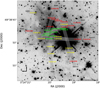 |
Fig. 2 HST F675W image with the slits and the [S II]/Hα ratio for each aperture overlaid. The green color corresponds to ratios above 0.4 within the error, the yellow color corresponds to ratios with a lower limit below 0.4, and the red color corresponds to apertures below 0.4 within the error. |
3.3 Other line ratios
We used other line ratios to verify the origin of the nebular emission around [W60] B90, including the ratios [O I]/Hα, [O II]/Hβ, [O III]/Hβ, [N II]/Hα, and [S II]/Hα. In Fig. D.1, we compare our measurements with the diagnostics presented in Kopsacheili et al. (2020). The diagnostics for all the apertures agree with a shocked scenario, except for [O III], which indicates a photoionized mechanism. This may be explained by the fact that the models in Kopsacheili et al. (2020) only apply to shocks with velocities between 100–1000 km s−1, while the peculiar velocity of [W60] B90 is ≤35 km s−1. Material ejected from the star at such a low velocity will not contain enough energy to ionize O II to O III. The presence of a nearby H II region at 14″ (LHA 120-N 132B; Henize 1956) and the newly discovered B1V star at 7″ (see Appendix C) could also explain the photoionized nature of [O III]. Radiation from nearby hot stars might contribute to the ionization of the gas around our RSG and cause the emission in areas with low [S II]/Hα. Even in the shocked areas, nebular emission might arise from a combination of shocks and photoionization from nearby hot stars. Another explanation for the inconsistency of [O III] is the brightness of the line. In all the apertures, the strength of [O III] λ5007 was approximately at the noise level (3σ detection), and therefore the fluxes might be underestimated, leading to lower ratios.
Mean radial velocity of the CSM.
3.4 Radial velocity of the CSM
We measured the RV of the CSM from the central wavelengths of the Balmer lines and forbidden emission lines detected (see Table B.2). We compared the RV of each ion at every location observed around [W60] B90. However, the difference in the RV among the apertures was smaller than the ±7 km s−1 error derived from the spectral resolution, preventing us from studying how the RVs are spatially distributed. We have, however, computed the median RV of each ion, using the individual velocities from each aperture (Table 2). We grouped the lines [S II] λλ6717, 6731 and [O II] λλ3726, 3729 to compute a single RV for [S II] and [O II], respectively. Given that the RV of [W60] B90 is 263.49 ± 1.02 km s−1 from Gaia DR3, we compared the kinematics of the nebular material to the kinematics of the star. All nebular lines are redshifted by ~10 km s−1 compared to the star, except for [S II] and [O I], which are ~20 km s−1 and ~40 km s−1, respectively. Each estimate is consistent with the low-velocity scenario (≤100 km s−1).
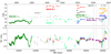 |
Fig. 3 Light curve of [W60] B90 indicating the respective survey and filter. Top: magnitudes obtained from each survey. Bottom: relative magnitude after subtracting the mean value of each data set. The vertical lines represent the epoch-spectroscopy as labeled in Table 1. |
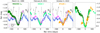 |
Fig. 4 Zoom in on the dimming events of [W60] B90. The first three panels show the comparison of the three dimmings of [W60] B90 with the Great Dimming of Betelgeuse (gray), the dimming of RW Cep (magenta), and a minimum from μ Cep (blue) in the V-band from AAVSO. The right panel overplots the photometry of the three dimmings of [W60] B90. We used the minimum of each data set as the zero-point reference for each graph. |
4 Variability of [W60] B90
4.1 Optical light curve
We assembled multi-epoch photometry of [W60] B90 from 1992 to the submission date of this work and we present the optical light curve in Fig. 3. We subtracted the mean value of each data set to obtain a relative magnitude, allowing for a comparison between different filters and surveys (see lower panel of Fig. 3). The amplitude of the ASAS-SN data is smaller than other surveys due to its pixel scale (8″px−1). Nearby sources are blended with [W60] B90, contaminating the data by adding a constant flux, which yields a lower amplitude. Nevertheless, we considered ASAS-SN as a guideline for the general shape of the light curve between 2017 and 2022, due to the lack of other data covering these years. After 2022, ATLAS and OGLE V-band provide better photometry due to their improved pixel scale (1.86 and 0.26″px−1, respectively).
We classify [W60] B90 as a semi-regular variable based on the short-period variability of Δm < 0.5 mag (Kiss et al. 2006), improving on the previous classifications: long-period variable (LPV; Gaia Collaboration 2023; Watson et al. 2006; Fraser et al. 2008) and nonperiodic variable (Jayasinghe et al. 2018). However, three exceptional events stand out with Δm ~ 1 mag and a rise time of ~400 d (Fig. 4). We present a comparison of the V-band from AAVSO of the Great Dimming of Betelgeuse, the recent dimming of RW Cep (Jones et al. 2023; Anugu et al. 2023) and the largest dimming (ΔV ~ 0.8 mag) of μ Cep in the last 50 yr, after the minimum in October 2015. We used the minimum of each event as the zero point for the relative magnitude and date. The first event in [W60] B90 occurred during the last years of the MACHO survey, between 1999 and 2000, reaching a minimum VKC = 15.4 mag and abruptly rising ΔVKC = 0.9 mag after. The next major event is identified in the OGLE V-band data between 2011 and 2012, when it suffered another dimming increasing ΔV = 0.9 mag, which was remarkably similar in time and brightness to the event in the MACHO data. The last major event occurred between October 2022 and November 2023, with the brightness increasing by Δc ~ 1.3 mag, Δo ~ 1 mag, and ΔV ~ 1.3 mag. However, this event has a small discontinuity in the rise, delaying the recovery compared to the other two events. The three events are 4350 and 4250 d apart, corresponding to an average recurrence period of approximately 11.8 years.
Apart from the three dimming events, we also note a variation in the photometric colors of [W60] B90 during three different minima in the light curve (Fig. 3). In general, a change to a redder color indicates a cooler atmospheric temperature, an increase in extinction due to dust formation, or both. The largest variation was observed by Gaia during the minimum in early 2015. BP − RP increased to 3.75 mag, as it faded, but stabilized around 3.45 mag after the recovery. Furthermore, the OGLE data revealed another change in color around 54100 MJD, when a large offset was observed between filters V and I. However, the poor sampling of the light curve prevents us from further analyzing this event. Lastly, the ATLAS c − o color increased during the 2022 minimum. Follow-up spectroscopic observations after the minimum revealed a decrease in the Teff and an enhancement of the extinction in agreement with the changing color (see Sect. 4.4). Remarkably, the color changes do not appear at every minimum, which suggests that specific conditions existed during these events.
4.2 Mid-infrared light curve
Extreme RSGs do not only show variability in the optical range but may also vary significantly at longer wavelengths. Yang et al. (2018) have found a correlation between the MIR variability, luminosity, and mass-loss rate, with the latter confirmed by Antoniadis et al. (2024). Therefore, we analyzed the NEOWISE data and compared it with the variability of [W60] B90 in the optical (Fig. 5). The long-term variability of the data agrees with the optical trend from the ASAS-SN photometry. Contrary to the optical data, no short-term variations were observed. For example, the ASAS-SN data shows a decrease in the brightness at 58 000 MJD, which is not detected in the NEOWISE bands. Higher cadence MIR photometry, as well as a comparison of optical to MIR photometry for other RSGs, is needed to confirm whether the short-term variations between the MIR and the optical are indeed decoupled.
The amplitude of the NEOWISE light curve is ΔW1 = 0.51 mag and ΔW2 = 0.37 mag. The data cover the last dimming event, yielding an amplitude ΔW1 = 0.42 mag and ΔW2 = 0.25 mag. We also calculated the median absolute deviation (MAD), a robust indicator to assess the variability, and found MADW1 = 0.0903 and MADW2 = 0.0918. Such a large MADW2 places [W60] B90 in the top four RSGs with the highest MADW2 in the LMC (see Fig. 17 in Yang et al. 2018). Hence, the large MIR variability agrees with the extreme nature of [W60] B90: one of the most luminous RSG in the LMC with the third highest mass-loss rate for a single RSG (Antoniadis et al. 2024).
 |
Fig. 5 Mid-infrared light curve of [W60] B90 from NEOWISE and Spitzer. W1 and [3.6] are shown with full and open blue circles, respectively; W2 and [4.5] are shown with full and open green squares. ASAS-SN data are shown in gray with an offset for comparison. |
4.3 Periodicity
Periods P1 = 1006 d and P2 = 453.44 ± 0.04 d have been derived using the MACHO data of [W60] B90 (Groenewegen et al. 2009; Groenewegen & Sloan 2018). Note that other studies reported P = 776 d (with ΔIc = 0.39 mag) from AAVSO photometry, and a long secondary period (LSP) of 4900 d, Δm = 0.12 mag from 50 yr of the digitized Harvard Astronomical Plate Collection (Watson et al. 2006; Chatys et al. 2019).
We used the period–luminosity (P-L) relations in the NIR and MIR (Yang & Jiang 2011) to calculate the predicted period and compare it with P1. We compiled the photometry of [W60] B90 in the bands J, H, Ks, [3.6], and [4.5] from the catalog of RSGs in the LMC published by Yang et al. (2018). We calculated the periods to be 829, 929, 1032, 1107, and 1041 d from J = 8.37, H = 7.40, Ks = 6.83, [3.6] = 6.29, and [4.5] = 6.29 mag, respectively. Despite the lack of error bars in P1 = 1006 d, we consider the derived periods from H, Ks, [3.6], and [4.5] consistent with the expected. In fact, Yang & Jiang (2011) mentioned that Ks and [3.6] are the most reliable bands to use their P-L relations as they are the least affected by extinction and provide the tightest relations. As they did not deredden the photometry, RSGs with high AV might differ from their predicted periods in the bands affected by extinction. Therefore, we attribute the shorter period from the J-band to the high extinction AV > 3 mag reported for [W60] B90 (see Sect. 4.4).
4.4 Optical spectroscopy
We compared the optical spectra of the four epochs presented in Fig. 6 to analyze the evolution of the star with time. We detect changes in the shape of the SED and the depth of the TiO bands throughout the epochs, implying a spectral-type variation from M3 I to M4 I. Changes in the SED imply either a variation in the Teff, E(B − V), or both. Since the metallicity Z of the star does not change, the strength of the TiO bands is exclusively related to the Teff (e.g., Levesque et al. 2007) and the wind of the star (Davies & Plez 2021), being deeper when the Teff is cooler and the wind is stronger. We used the grid of MARCS models described in de Wit et al. (2023) to obtain the physical parameters for each spectral epoch. We primarily fit for Teff and E(B − V), keeping Z and log(g) fixed from the results in the J-band (see Sec. 4.6). We derived Z = −0.25 dex and log(g) = +0.5 dex from the local thermodynamic equilibrium (LTE) MARCS models, in contrast to de Wit et al. (2023), who assumed a LMC-like metallicity (Z = −0.38 dex) and obtained log(g) = −0.2 dex from the Ca II triplet. The discrepancy in log(g) does not affect our fit in the optical as the TiO bands are temperature indicators and not sensitive to gravity. Finally, we performed the fitting in two stages. In the first iteration, we fitted spectral regions including shorter wavelengths to constrain the shape of the SED and get more accurate values for E(B − V). Then, fixing E(B − V) in the second iteration, we only use spectral regions affected by the TiO bands to obtain the Teff of the star. The best-fit models to each epoch are shown in Fig. 7 and their parameters are shown in Table 3.
We obtained Epoch1 at the beginning of 2020 when the RSG exhibited low-amplitude variability (see Fig. 3). Indeed, the fit of Epoch1 reveals the lowest χ2 among our sample, implying minor deviations from the model spectra, suggesting the RSG atmosphere was stable. During the following years (2020–2022), the brightness decreased Δg = 0.3 mag in ASAS-SN, although the real change in brightness might be larger (see discussion in Sec. 4.1). We obtained Epoch2 two months after the photometric minimum. This spectrum reveals the strongest TiO bands of all epochs, implying either a decrease in the Teff, an increase of ![Mathematical equation: $\[\dot{M}\]$](/articles/aa/full_html/2024/10/aa50737-24/aa50737-24-eq6.png) , or a combination of both. The spectrum suggests a complex atmospheric structure following the photometric minimum, which cannot be reproduced by a single MARCS model (see Sec. 4.5), and we consider the Teff and the E(B − V) derived for Epoch2 to be unreliable. We obtained Epoch3 four months later, when the RSG exhibited a plateau during the recovery, after initially increasing Δo = 0.5 mag compared to the minimum. It shows weaker TiO bands than Epoch2, and we found a higher best-fit Teff according to this change. However, E(B − V) is considerably higher than the previous epochs, implying that the extinction in the line of sight increased after the minimum. Finally, we obtained Epoch4 two months before the maximum in late 2023. In this epoch, it was brighter than Epoch2 by Δo = 0.9 mag, and the RSG exhibited the highest measured Teff. The SED is not as extinct as in Epoch3 but is steeper than in the first two spectra, in agreement with the derived E(B − V).
, or a combination of both. The spectrum suggests a complex atmospheric structure following the photometric minimum, which cannot be reproduced by a single MARCS model (see Sec. 4.5), and we consider the Teff and the E(B − V) derived for Epoch2 to be unreliable. We obtained Epoch3 four months later, when the RSG exhibited a plateau during the recovery, after initially increasing Δo = 0.5 mag compared to the minimum. It shows weaker TiO bands than Epoch2, and we found a higher best-fit Teff according to this change. However, E(B − V) is considerably higher than the previous epochs, implying that the extinction in the line of sight increased after the minimum. Finally, we obtained Epoch4 two months before the maximum in late 2023. In this epoch, it was brighter than Epoch2 by Δo = 0.9 mag, and the RSG exhibited the highest measured Teff. The SED is not as extinct as in Epoch3 but is steeper than in the first two spectra, in agreement with the derived E(B − V).
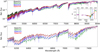 |
Fig. 6 Comparison of the spectroscopic epochs of W60 [B90] in the optical (top) and the main TiO bands at 6150 and 7050 Å (bottom). The inset shows the light curve (as in Fig. 3) indicating each spectroscopic epoch with the dashed lines, following the color code of the spectra. |
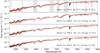 |
Fig. 7 Best MARCS model fit (red) for each epoch from MagE (black). Shaded areas in Epoch 1 show the spectral regions used in the fitting. |
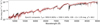 |
Fig. 8 Comparison between the best composite model (red), with 60% of the flux from a single Teff1 = 3950 K and 40% from Teff2 = 3300 K, and the best single model (gray) from Fig. 7 for Epoch 2. |
Physical parameters of [W60] B90 from spectroscopy.
4.5 Spectroscopy during the dimming (Epoch2)
The Great Dimming of Betelgeuse was explained by a clump of dust in the line of sight or, alternatively, a cold patch in the atmosphere (Montargès et al. 2021). We attempted to model the latter by creating a grid of composite MARCS models. We created composite models from the superposition of two single models (Teff1 and Teff2) with weighted fluxes from each model in steps of 20% (e.g., 80–20% or 60–40%). We used Teff from 3300–4500 K in steps of 50 K and assumed Z = −0.25 dex and log(g) = −0.2 dex as in Sec. 4.4.
We obtained the best fit for 60% of Teff1 = 3300 K, 40% of Teff2 = 4500 K, E(B − V) = 1.2 mag, and χ2 = 62.4. The composite model considerably improves the fit, but the temperatures found are at the edges of the grid. Fixing Teff1 = 3950 K using the result of EpochJ (see Sec. 4.6), we derived the best fit for 60% of Teff1 = 3950 K to be 40% of Teff2 = 3300 K and E(B − V) = 1.25 mag, with a χ2 = 68.2 (Fig. 8), again finding a Teff2 at the edge of the grid. Nevertheless, we argue that the MARCS models cannot always reproduce the real photosphere of an extreme RSG. Physical processes such as 3D assumptions, wind, or magnetic fields, are currently missing in the MARCS models recipes. Hence, a new generation of models including these processes is needed to properly reproduce the complete nature of RSGs.
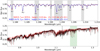 |
Fig. 9 Derived parameters from the FIRE spectrum. Top: best fit of the FIRE spectrum (solid black) in the J-band for the LTE MARCS models (dashed-dot red) and the NLTE-corrected version (solid blue) with the NLTE effects applied to the indicated lines. The spectral regions used in the fitting are shown with gray shades. Bottom: best LTE MARCS model (dotted red) from the J-band to the FIRE spectrum (black). The model was reddened with E(B − V) = 1.05 mag to match the SED. The green-shaded region highlights the spectral region shown in the upper plot. |
4.6 Near-infrared spectroscopy
We applied the nonLTE (NLTE) MARCS models (Bergemann et al. 2012, 2013, 2015) to fit the atomic lines in the J-band of our FIRE spectrum. We created a grid of models with a range Teff= 3300–4500 K in steps of 25 K, log(g) = −0.5, +0.5 dex in steps of 0.25 dex, microturbulent velocities from 2.5 to 5.5 km s−1 in steps of 0.5 km s−1 and Z = −0.38, −0.25, −0.1, +0.0 and + 0.2 dex. Also, we used the LTE grid presented in the previous section to compare the results from the NLTE models with the canonical MARCS models. We found the best-fit model with reduced χ2 and the uncertainties from the 1σ interval of the distribution. We followed the approach presented in Patrick et al. (2017) and fitted the lines Fe I λλ1.178327, 1.188285, 1.197305, Si I λλ1.198419, 1.199157, 1.203151, Mg I λλ1.208335 and Ti I λλ1.189289, 1.194954. We excluded the line Mg I λλ1.182819 because the feature on the right wing of the line profile is not in the models and could compromise the diagnostic of the line. Similarly, we rejected Si I λλ1.210353 due to the difficulty of establishing the continuum level during the fit. Nevertheless, both lines are satisfactorily reproduced by the best-fit model probing that their rejection did not compromise the result.
The results presented in Fig. 9 and Table 3 show a strong disagreement of ≳300 K between the Teff derived from the TiO bands (Teff,TiO) in the optical spectra and the atomic lines fit in the J-band (Teff,J). The NLTE models constrain the Teff,J better than the LTE models, although both results are consistent within the errors. Both indicate higher Z than the commonly Z = −0.38 dex assumed for the LMC, with the LTE models suggesting a slightly higher Z than the LMC, while the NLTE models favor a solar Z. The log(g) results are poorly constrained as the errors span over the whole range of the grid. The best NLTE model finds log(g) = ![Mathematical equation: $\[+0.50_{-0.75}^{+0.00}\]$](/articles/aa/full_html/2024/10/aa50737-24/aa50737-24-eq21.png) dex, similar to what de Wit et al. (2023) derived from the Ca II triplet in Epoch1 and consistent within error with the LTE result log(g) =
dex, similar to what de Wit et al. (2023) derived from the Ca II triplet in Epoch1 and consistent within error with the LTE result log(g) = ![Mathematical equation: $\[-0.2_{-0.30}^{+0.20}\]$](/articles/aa/full_html/2024/10/aa50737-24/aa50737-24-eq22.png) dex as the best solution. We applied log(g) and Z from the LTE result to constrain the physical parameters in the optical for consistency, as the TiO bands do not have NLTE correction (see Sec. 4.4). Therefore, using Z = +0.00 from the NLTE in the optical instead of Z = −0.25 would lead to an overestimation of the abundances, affecting the Teff,TiO. However, the discrepancy in log(g) between the LTE and the NLTE result is negligible as the TiO bands are not sensitive to this parameter.
dex as the best solution. We applied log(g) and Z from the LTE result to constrain the physical parameters in the optical for consistency, as the TiO bands do not have NLTE correction (see Sec. 4.4). Therefore, using Z = +0.00 from the NLTE in the optical instead of Z = −0.25 would lead to an overestimation of the abundances, affecting the Teff,TiO. However, the discrepancy in log(g) between the LTE and the NLTE result is negligible as the TiO bands are not sensitive to this parameter.
5 Discussion
5.1 Bow shock, bar and runaway status
Only three single Galactic RSGs with a bow shock have been identified so far: Betelgeuse, IRC-10414, and μ Cep, with only the bow shock of IRC-10414 being visually detected in the optical range. An analysis of [S II]/Hα revealed a ratio of 0.3 (Gvaramadze et al. 2014), which is even lower than the values reported around [W60] B90. Among the three RSGs, only Betelgeuse exhibits a bar, which is located at 0.5 pc from the star (assuming a distance of 200 pc; Harper et al. 2008, 2017) and which remains unexplained. It might be the relic of the blue supergiant (BSG) wind interaction with the ISM, just before Betelgeuse recently became a RSG (Mackey et al. 2012). Although new constraints on the evolutionary status of Betelgeuse reject this hypothesis, and an interstellar origin was proposed instead (Decin et al. 2012; Meyer et al. 2021). The bar could be the edge of an interstellar cloud illuminated by Betelgeuse or a linear filament in the interstellar cirrus. Some efforts have been made to detect the bar and the bow shock in the optical with no success. The glow prevented the detection of the bar through imaging even setting the star outside the field of view (private communication with Dr. Jonathan Mackey). In the case of [W60] B90, the bar structure at 1 pc is partially shocked, but only in the southeastern part. The movement of [W60] B90 towards the bar and the shocked material found between them and in the bar confirms a causal connection. However, the interpretation of our findings requires further work and is beyond the scope of this paper.
[W60] B90 moves towards the bar with a peculiar velocity between 16 and 25(±11) km s−1 (Table A.1). Given that hydrogen is the most abundant element in the gas, we can assume that it is a good tracer of the CSM and use the ~10 km s−1 difference in RV between Hα and the star to construct the 3D velocity. Therefore, [W60] B90 moves with a 19–27(±11) km s−1 velocity, establishing it as a walkaway star, on the brink of the runaway limit (>30 km s−1; Renzo et al. 2019). The speed of sound in the low-density isothermal warm neutral medium is on the order of ~1 km s−1 (Cox et al. 2012). Therefore, the RSG would move supersonically in the medium even considering the 3D lower limit of 8 km s−1. Studies of the case of Betelgeuse demonstrated that lower velocities than 50 km s−1 can produce an observable bow shock during ~100 kyr, a significant fraction of the post-main sequence evolution (Mackey et al. 2012). Also, bow shocks with low stellar velocities form clumpy substructures due to Kelvin-Helmholtz instabilities, which could explain why we do not measure homogeneous [S II]/Hα values around the star (Mohamed et al. 2012).
Further releases from Gaia will improve the uncertainties on the peculiar velocity, allowing us to trace back its movement, discern its birthplace, and speculate the cause of its ejection, either by dynamical interactions or from a SN kick (Stoop et al. 2023).
Apart from detecting shocked material where the bow shock is expected, we also find enhanced [S II]/Hα at northern positions close to the star. This might indicate an inhomogeneous CSM and clumpy, asymmetric mass-loss events. Observations in the MIR have shown multiple arcs and similarly strong asymmetries in the CSM of Betelgeuse. Decin et al. (2012) demonstrated that a combination of anisotropic mass-loss processes and the influence of galactic magnetic fields might explain the multiple arcs and clumps around Betelgeuse. Further observations are needed to spatially resolve the circumstellar environment of [W60] B90. Identifying the hypothesized bow shock or inhomogeneous structures around the star would help to constrain the recent mass-losing history of [W60] B90.
5.2 Properties of the dimming events
Our spectroscopic analysis revealed physical properties similar to those of Betelgeuse during the Great Dimming (see Sects. 4.5 and 5.3), therefore, we speculate that the same physical mechanism drives both events. MacLeod et al. (2023) explained the Great Dimming as a result of a hot convective plume that forms in the turbulent envelope, breaking free from the surface and triggering a mass ejection. However, the Great Dimming displayed a more abrupt brightness rise on a shorter timescale (~200 d) than the rise of the events of our RSG (~400 d). The radius of [W60] B90 is ~1200 R⊙, while that of Betelgeuse is reported to be between 750–1000 R⊙ (Joyce et al. 2020; Kravchenko et al. 2021). Contrarily, μ Cep (1259 R⊙; Josselin & Plez 2007) and the Galactic hypergiant RW Cep (900–1760 R⊙; Anugu et al. 2023) have a comparable radius to [W60] B90, and both stars exhibit a similar rise after the minima (Fig. 4). The large uncertainty in the radius of RW Cep derives from the large uncertainty in the distance and, hence, luminosity. We speculate that the timescale of these events is related to the radius of the stars, as a more extended atmosphere needs more time to stabilize. A similar idea was already presented in the analysis of the dimming of RW Cep (Anugu et al. 2023), but it needs to be tested with more dimming events in RSGs. However, assuming a similar timescale in the recovery of RW Cep with respect to μ Cep and [W60] B90, would constrain the radius of RW Cep to ~1200 R⊙. The dimming events of [W60] B90 have a recurrence of ~11.8 yr, while the dimming of μ Cep is unique over the past 50 yr and the Great Dimming of Betelgeuse is unique over the last 100 yr. Only one dimming event has been observed for RW Cep, but the dust shells detected around the hypergiant suggest that it may have undergone several mass ejections over the last century (Anugu et al. 2023; Jones et al. 2023). Moreover, the rising plume on Betelgeuse disturbed its pulsation period, switching from the ~400 d fundamental period to the ~200 d overtone (MacLeod et al. 2023). We do not find a change in the periodicity in any of the three dimmings.
VY CMa is another red hypergiant that experienced several dimming events during the last century. The most extreme event occurred in the 90s when the star decreased the brightness by ~ 3 mag. The other events showed variations of Δm ~ 1.5 mag (Humphreys et al. 2020) which are still larger than the events of [W60] B90 (Δm ~ 1 mag). Moreover, the ~500 d rise time on the VY CMa is larger than the ~400 d of [W60] B90, which agrees with VY CMa having a bigger size (1420 ± 120 R⊙; Wittkowski et al. 2012) than [W60] B90 (~1200 R⊙). Different gaseous knots, arcs, and irregular structures surrounding VY CMa have been identified as discrete mass ejections related to each minimum during the last century. These massive gaseous outflows explain the high mass loss of VY CMa (Humphreys et al. 2005, 2007, 2020). On the other hand, although similar structures have been identified around Betelgeuse, they do not explain the overall mass-loss rate of this RSG but contribute to it (Humphreys et al. 2024). Spatially resolving the CSM of [W60] B90 could reveal the presence of gaseous structures, show if there is a correlation with the 11.8 yr recurrence of the dimmings, and if they explain the mass-loss rate as in VY CMa or only contribute to it as in Betelgeuse. Extending the long-term variability study to other luminous RSGs is needed to understand how common such events are, and confirm their dependence on the size of the RSG.
The fundamental period P1 = 1006 d (Groenewegen & Sloan 2018) and the 4900 d LSP of [W60] B90 are considerably larger than the fundamental P ~ 400 d (Kiss et al. 2006) and the 2000–2365 d LSP (Chatys et al. 2019; Joyce et al. 2020) of Betelgeuse. They are also consistent with the expected P from the P-L relations and the higher luminosity of [W60] B90. Although Chatys et al. (2019) do not provide errors, their 13.5 yr LSP of [W60] B90 is suspiciously close to the 11.8 yr of the dimming recurrence found in this paper. Furthermore, the periods found in [W60] B90 are remarkably similar to the fundamental period P=880 d and LSP of 4400 d of μ Cep. Although this RSG is reported to be comparable in luminosity and radius to [W60] B90 (see Sec. 5.6), no recurrence of dimming events has been reported in μ Cep to date.
5.3 Spectral variability
The TiO bands are the primary spectroscopic feature for classifying M-stars in the optical. Dorda et al. (2016) found that 30% of the ~500 RSGs in their LMC sample showed spectral type variability with a mean change of two spectral subtypes. They also reported that cool RSGs are more likely to exhibit spectral-type changes. In the case of [W60] B90, we found the depth of the TiO bands to vary among the epochs, yielding a spectral type of M3 I in Epoch1 (de Wit et al. 2023) and M4 I in Epoch2. However, observations of the star during its maximum and minimum would likely yield larger spectral variability. These results demonstrate the uncertainty of spectroscopically classifying variable RSGs based on a single observation.
A tomographic analysis of μ Cep and Betelgeuse explained the correlation between Teff,TiO and the optical variability as an effect of the convective cells in the atmosphere (Kravchenko et al. 2019, 2021). The Teff,TiO and the brightness decrease as the material rises, while both increase once it falls, creating a hysteresis loop between the RV of the atomic lines and the Teff,TiO. We report a similar trend between Teff,TiO and the optical variability for [W60] B90 during the brightening in 2022. The Epoch2 spectrum was obtained 2 months after the minimum in 2022, showing spectral features incompatible with single MARCS models. Montargès et al. (2021) explained the Great Dimming as a large cold spot rising in the atmosphere of Betelgeuse. Big convective cells at different temperatures can create large cold spots that cause deeper TiO bands, decreasing the brightness in the optical. Furthermore, if convection is strong enough, it can result in a mass ejection (MacLeod et al. 2023; Drevon et al. 2024). This scenario is consistent with the enhanced extinction reported in the epochs following the minimum Epoch3 and Epoch4, where AV changes from 3.41 ± 0.51 mag before the event to ![Mathematical equation: $\[4.60_{-0.17}^{+0.34}\]$](/articles/aa/full_html/2024/10/aa50737-24/aa50737-24-eq23.png) mag several months after. This demonstrates the importance of using the light curve to interpret whether the RSG was observed during a stable state, or during a brief minimum or maximum. Further investigation is needed to reveal the origin of the hysteresis loops and how they are related to episodic mass-loss events.
mag several months after. This demonstrates the importance of using the light curve to interpret whether the RSG was observed during a stable state, or during a brief minimum or maximum. Further investigation is needed to reveal the origin of the hysteresis loops and how they are related to episodic mass-loss events.
5.4 Teff,TiO versus Teff,J
We found a strong discrepancy in Teff when we obtained the physical parameters from different spectral ranges. While the TiO bands in the optical suggest Teff,TiO ≈ 3550 K, we derived Teff,J = 3900 K from the atomic lines in the J-band. Davies et al. (2013, 2015) already reported a discrepancy in Teff derived from the TiO bands compared with the J-band or the SED fits, which is related to the formation zone of each diagnostic. However, if the MARCS models were consistent, one single model would describe the atmosphere of the star with one single Teff. Given these discrepancies, de Wit et al. (2024) derived a Teff scaling relation based on the MARCS models to scale Teff,TiO to a more secure Teff. Using their relation, we find Teff,J = 3960 K, which is consistent with our results.
Previous studies on luminous RSGs have also reported very cool Teff,TiO, which cannot be reproduced by the theoretical evolutionary models (e.g., Levesque et al. 2007; de Wit et al. 2024). Davies & Plez (2021) demonstrated that adding a ![Mathematical equation: $\[\dot{M}\]$](/articles/aa/full_html/2024/10/aa50737-24/aa50737-24-eq24.png) to the MARCS models results in an enhancement in the TiO band strengths, similar to the effect of decreasing the Teff. The Teff,TiO, therefore, might be underestimated in evolved luminous RSGs with strong
to the MARCS models results in an enhancement in the TiO band strengths, similar to the effect of decreasing the Teff. The Teff,TiO, therefore, might be underestimated in evolved luminous RSGs with strong ![Mathematical equation: $\[\dot{M}\]$](/articles/aa/full_html/2024/10/aa50737-24/aa50737-24-eq25.png) as the MARCS models do not account for it. Recently, by implementing
as the MARCS models do not account for it. Recently, by implementing ![Mathematical equation: $\[\dot{M}\]$](/articles/aa/full_html/2024/10/aa50737-24/aa50737-24-eq26.png) to the MARCS models, González-Torà et al. (2024) were able to reconcile spectral features in the near and MIR that did not match with the canonical MARCS models. Our results reinforce the urgent need for a complete grid of models with
to the MARCS models, González-Torà et al. (2024) were able to reconcile spectral features in the near and MIR that did not match with the canonical MARCS models. Our results reinforce the urgent need for a complete grid of models with ![Mathematical equation: $\[\dot{M}\]$](/articles/aa/full_html/2024/10/aa50737-24/aa50737-24-eq27.png) to break the degeneracy in the optical and reconcile the Teff,TiO, the Teff,J and the evolutionary models. Extending the 1D LTE assumptions from the MARCS models to 3D magneto-hydrodynamic ones will also improve the modeling of the strong convection in RSGs (e.g., Kravchenko et al. 2019; Ma et al. 2024).
to break the degeneracy in the optical and reconcile the Teff,TiO, the Teff,J and the evolutionary models. Extending the 1D LTE assumptions from the MARCS models to 3D magneto-hydrodynamic ones will also improve the modeling of the strong convection in RSGs (e.g., Kravchenko et al. 2019; Ma et al. 2024).
Furthermore, the addition of NLTE corrections to the MARCS models for the atomic lines in the J-band considerably impacts the results. It decreases the uncertainty in Teff and it reveals a high metallicity ![Mathematical equation: $\[\left(Z=+0.00_{-0.10}^{+0.20} ~\mathrm{dex}\right)\]$](/articles/aa/full_html/2024/10/aa50737-24/aa50737-24-eq28.png) , which is inconsistent with the mean metallicity of the LMC (Z = 0.37 ± 0.14 dex; Davies et al. 2015). Although it is more metal-rich than expected for the LMC, [W60] B90 is not the first cool supergiant with solar-like Z, as six more cases are already known in the LMC (Tabernero et al. 2018). The solar Z, however, is in conflict with the low-Z environment suggested by the faint nitrogen nebular emission. The enhanced Z can be explained by extra rotational mixing occurring in its interior during its evolution enhancing the metal content in the surface, by a binary history with mass-transfer changing the abundances, or even a merger with a companion.
, which is inconsistent with the mean metallicity of the LMC (Z = 0.37 ± 0.14 dex; Davies et al. 2015). Although it is more metal-rich than expected for the LMC, [W60] B90 is not the first cool supergiant with solar-like Z, as six more cases are already known in the LMC (Tabernero et al. 2018). The solar Z, however, is in conflict with the low-Z environment suggested by the faint nitrogen nebular emission. The enhanced Z can be explained by extra rotational mixing occurring in its interior during its evolution enhancing the metal content in the surface, by a binary history with mass-transfer changing the abundances, or even a merger with a companion.
Radial velocity of Ca II triplet.
5.5 Binarity
Recent works have estimated the fraction of RSGs in binary systems to be at least 15% (Dorda & Patrick 2021; Patrick et al. 2022). We explored the RV variations from the Ca II triplet (Table 4) and found all epochs to be consistent with the Gaia DR3 value, except for Epoch3. We cannot attribute the difference of less than 10 km s−1 to the presence of a companion, as tomographic studies have revealed that such variations can be explained by the rising and falling of material in the atmosphere (Kravchenko et al. 2019, 2021). A pilot study by Patrick (2020) suggested a correlation between the RV variations and the luminosity of the RSGs, which might be connected to stronger hysteresis loops. Since [W60] B90 is close to the observed upper luminosity of RSGs in the LMC (Davies et al. 2018), it is expected to have larger variability and RV differences. Therefore, we argue that the small discrepancy in the RV is a combined effect of the changes in the atmosphere due to its evolutionary status and the intrinsic error of ±7 km s−1 from the observations. Moreover, Gaia DR3 indicators such as the RUWE, astrometric excess noise, and binary probability parameter do not support a binary scenario. We also report the absence of a counterpart in Swift observations and the nondetection of blue excess in the SED, disfavouring a hot companion. Therefore, we conclude that [W60] B90 is currently a single star given the total lack of evidence for a companion.
5.6 Mass-loss rates
Antoniadis et al. (2024) determined the mass-loss rates of over 2000 RSGs in the LMC using the radiative transfer code DUSTY, finding ![Mathematical equation: $\[\dot{M}=5.1_{-1.7}^{+5.1} \times 10^{-6} ~\mathrm{M}_{\odot} ~\mathrm{yr}^{-1}\]$](/articles/aa/full_html/2024/10/aa50737-24/aa50737-24-eq29.png) for [W60] B90. In this work, we recomputed the
for [W60] B90. In this work, we recomputed the ![Mathematical equation: $\[\dot{M}\]$](/articles/aa/full_html/2024/10/aa50737-24/aa50737-24-eq30.png) with identical assumptions, but including synthetic photometry from the IRS spectrum (see Sect. 2.4) to improve the SED fitting. We present the new fit in Fig. 10, which results in
with identical assumptions, but including synthetic photometry from the IRS spectrum (see Sect. 2.4) to improve the SED fitting. We present the new fit in Fig. 10, which results in ![Mathematical equation: $\[\dot{M}=4.4_{-1.7}^{+5.1} \times 10^{-6} ~\mathrm{M}_{\odot} ~\mathrm{yr}^{-1}\]$](/articles/aa/full_html/2024/10/aa50737-24/aa50737-24-eq31.png) with a best-fit optical depth τV = 1.76 for the best fit of Teff = 3300 K and inner dust shell temperature Tin = 1200 K (for the description of the fitted parameters see Antoniadis et al. 2024). This
with a best-fit optical depth τV = 1.76 for the best fit of Teff = 3300 K and inner dust shell temperature Tin = 1200 K (for the description of the fitted parameters see Antoniadis et al. 2024). This ![Mathematical equation: $\[\dot{M}\]$](/articles/aa/full_html/2024/10/aa50737-24/aa50737-24-eq32.png) makes [W60] B90 the third highest mass-losing probably single RSG in the Antoniadis et al. (2024) sample. Moreover, it is the second highest
makes [W60] B90 the third highest mass-losing probably single RSG in the Antoniadis et al. (2024) sample. Moreover, it is the second highest ![Mathematical equation: $\[\dot{M}_{\text {dust }}\]$](/articles/aa/full_html/2024/10/aa50737-24/aa50737-24-eq33.png) among the oxygen-rich stars in the study of evolved stars in the LMC from Riebel et al. (2012). These results underline the extreme nature of [W60] B90 and agree with it being one of the most variable RSGs in the MIR in the LMC (Yang et al. 2018).
among the oxygen-rich stars in the study of evolved stars in the LMC from Riebel et al. (2012). These results underline the extreme nature of [W60] B90 and agree with it being one of the most variable RSGs in the MIR in the LMC (Yang et al. 2018).
From the properties of a bow shock, one can derive the mass-loss rate of the producer. Therefore, we compare the mass-loss rate and the general properties of [W60] B90 with the three known, Galactic RSGs with a bow shock in Table 5. All of them have considerable mass-loss (![Mathematical equation: $\[\dot{M}\]$](/articles/aa/full_html/2024/10/aa50737-24/aa50737-24-eq36.png) > 10−6 M⊙ yr−1) and high luminosity (log(L/L⊙) > 5.0 dex). IRC-10414 and μ Cep are fast runaways, while Betelgeuse is at the limit between a walkaway and a runaway star. Remarkably, Betelgeuse is the most compact of the RSGs, exhibiting shorter periods, while [W60] B90 and μ Cep have comparable periodicity (see Sect. 5.2). However, none of the physical properties stand out as a common signature of a bow shock. External factors to the RSGs such as their environment or the specific evolution likely determine the formation of a bow shock.
> 10−6 M⊙ yr−1) and high luminosity (log(L/L⊙) > 5.0 dex). IRC-10414 and μ Cep are fast runaways, while Betelgeuse is at the limit between a walkaway and a runaway star. Remarkably, Betelgeuse is the most compact of the RSGs, exhibiting shorter periods, while [W60] B90 and μ Cep have comparable periodicity (see Sect. 5.2). However, none of the physical properties stand out as a common signature of a bow shock. External factors to the RSGs such as their environment or the specific evolution likely determine the formation of a bow shock.
Parameters of [W60] B90 compared to the three known RSGs with a bow shock.
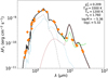 |
Fig. 10 SED of [W60] B90. The orange diamonds show the observations and the black line is the best-fit model from DUSTY, which is a superposition of attenuated flux (dashed light blue), the scattered flux (dot-dashed gray), and dust emission (dotted brown). The green curve represents the Spitzer IRS spectrum. |
 |
Fig. 11 Location of [W60] B90 (red triangle) in the Hertzsprung-Russell diagram of the RSG population in the LMC (black dots, Yang et al. 2021). The color map represents the central 12C mass fraction on the MIST evolutionary track, while the nodes indicate a step of 104 yr. |
5.7 Evolutionary status
We explore the location of [W60] B90 in the Hertzsprung-Russell diagram in Fig. 11 by using the derived Teff,J = ![Mathematical equation: $\[3900_{-100}^{+150}\]$](/articles/aa/full_html/2024/10/aa50737-24/aa50737-24-eq37.png) K (see Table 3) and log(L/L⊙) = 5.32 ± 0.01 dex (Antoniadis et al. 2024). Similar to de Wit et al. (2023), we compare its location to the LMC catalog of RSGs from Yang et al. (2021). We also used the MIST models (Dotter 2016; Choi et al. 2016) of rotating single stars (υ; = 0.4υ;crit) in the range of 8 to 25 M⊙. The position of [W60] B90 consistently matches the initial mass Mini = 25 M⊙ track, being more massive than Betelgeuse (Mini = 18–21; Joyce et al. 2020), with current carbon burning in the core and within the last two nodes of the evolutionary track. Therefore, following the expected evolution for a RSG, [W60] B90 should explode as a Type II SN within the next 104 yr (Smartt et al. 2009). However, the observational lack of massive RSGs exploding as SNe (the so-called ‘RSG problem’; Smartt 2009, 2015) suggests that either they end their lives in warmer states by stripping part of their envelopes or they collapse into black holes without exploding. Although determining the future evolution of [W60] B90 is beyond the scope of this paper, monitoring this evolved massive RSG could shed light on the “RSG problem” and indicate whether episodic mass-loss influences the fate of RSGs.
K (see Table 3) and log(L/L⊙) = 5.32 ± 0.01 dex (Antoniadis et al. 2024). Similar to de Wit et al. (2023), we compare its location to the LMC catalog of RSGs from Yang et al. (2021). We also used the MIST models (Dotter 2016; Choi et al. 2016) of rotating single stars (υ; = 0.4υ;crit) in the range of 8 to 25 M⊙. The position of [W60] B90 consistently matches the initial mass Mini = 25 M⊙ track, being more massive than Betelgeuse (Mini = 18–21; Joyce et al. 2020), with current carbon burning in the core and within the last two nodes of the evolutionary track. Therefore, following the expected evolution for a RSG, [W60] B90 should explode as a Type II SN within the next 104 yr (Smartt et al. 2009). However, the observational lack of massive RSGs exploding as SNe (the so-called ‘RSG problem’; Smartt 2009, 2015) suggests that either they end their lives in warmer states by stripping part of their envelopes or they collapse into black holes without exploding. Although determining the future evolution of [W60] B90 is beyond the scope of this paper, monitoring this evolved massive RSG could shed light on the “RSG problem” and indicate whether episodic mass-loss influences the fate of RSGs.
6 Summary and conclusions
We present a detailed study of the very luminous RSG [W60] B90 (log(L/L⊙) = 5.32 dex), motivated by the discovery of a bar-like structure at 1 pc, which is reminiscent of the bar around Betelgeuse. We found [W60] B90 to be a walkaway star, with a supersonic peculiar velocity between 16–25 (±11) km s−1 in the direction of the bar. We also obtained optical long-slit spectroscopy of the circumstellar environment of [W60] B90 to search for evidence of the hypothesized bow shock. We used the criterion [S II]/Hα> 0.4 to reveal the shocked origin of the nebular emission in the southern part of the bar, which confirms a causal connection with the RSG, and between the bar and the star, where the bow shock is expected. Therefore, [W60] B90 is the first extragalactic RSG with a suspected bow shock.
We compiled archival photometry to construct an optical light curve spanning more than 30 yr, reporting three dimming events in the optical with a recurrence of ~11.8 yr and ΔV ~1 mag. We note a similar recovery timescale of ~400 d for each dimming event in [W60] B90, in contrast with the Great Dimming of Betelgeuse, which lasted ~200 d. We attribute the delay in the recovery to the size of the atmosphere, as [W60] B90 is more extended than Betelgeuse and the adjustment within the atmosphere needs additional time to manifest. We support this argument by reporting similarities in the timescale between the dimmings of [W60] B90 with those of μ Cep and the hypergiant RW Cep (Anugu et al. 2023), which are comparable in size to our RSG. We also assemble a 10 yr MIR light curve reporting a general amplitude ΔW1 = 0.51 mag and ΔW2 = 0.37 mag, a variation ΔW1 = 0.42 mag and ΔW2 = 0.25 mag during the last dimming event, and a long-term variability correlation with the optical.
Optical multi-epoch spectroscopy during the recovery of the last dimming event revealed different atmospheric properties for each epoch and spectral variability (from M3 I to M4 I), highlighting the importance of light curves in assessing the current state of variable RSGs. We note a correlation correlation between the Teff,TiO and the brightness of the star, which might be connected to convection (Kravchenko et al. 2019, 2021). We detect an enhancement of AV after the dimming, which suggests an addition of dust in the line of sight, as a consequence of a mass ejection during the minimum. In addition, a single model cannot reproduce the complex atmosphere of the star during the closest epoch to the minimum. A composite model of cool and hot components considerably improves the description of the spectral features observed. We conclude that [W60] B90 suffered a mass ejection similar to that reported during the Great Dimming of Betelgeuse (Montargès et al. 2021; Dupree et al. 2022) and the dimming of RW Cep (Anugu et al. 2023). Furthermore, we find solar-like metallicity ![Mathematical equation: $\[Z=0.0_{-0.1}^{+0.2}\]$](/articles/aa/full_html/2024/10/aa50737-24/aa50737-24-eq38.png) dex from the atomic lines in the J-band, which might indicate the evolved state of [W60] B90 and prior mixing in the stellar interior entailing an overabundance of metals on the surface. We also report incompatible differences of ΔTeff > 300 K between the diagnostic in the J-band and the optical TiO bands. New models are urgently needed as the current ones are inconsistent depending on the spectral range observed. Further studies are needed in order to construct the new generation of RSG models, allowing further constraint of the basic properties of RSGs such as NLTE assumptions, the wind of the star, convection, and magnetic fields.
dex from the atomic lines in the J-band, which might indicate the evolved state of [W60] B90 and prior mixing in the stellar interior entailing an overabundance of metals on the surface. We also report incompatible differences of ΔTeff > 300 K between the diagnostic in the J-band and the optical TiO bands. New models are urgently needed as the current ones are inconsistent depending on the spectral range observed. Further studies are needed in order to construct the new generation of RSG models, allowing further constraint of the basic properties of RSGs such as NLTE assumptions, the wind of the star, convection, and magnetic fields.
The detection of shocked material in the CSM, the high mass-loss rate ![Mathematical equation: $\[\left(\dot{M}=4.4_{-1.7}^{+5.1} \times 10^{-6} ~\mathrm{M}_{\odot} ~\mathrm{yr}^{-1}\right)\]$](/articles/aa/full_html/2024/10/aa50737-24/aa50737-24-eq39.png) , the high variability reported in the optical and the MIR, and the changes in the extinction after the minimum in 2022 suggest that [W60] B90 is in an unstable evolutionary state and is undergoing episodes of mass loss. Its location in the Hertzsprung-Russell diagram is a good match with the Mini = 25 M⊙ MIST evolutionary models within the last 104 yr before the end of its life. This work reveals [W60] B90 to be a perfect laboratory with which to study episodic mass loss in evolved RSGs at low-Z environments. Despite our detailed analysis, further investigation is needed to shed more light on the system. Observations with high spatial resolution, for example with ALMA or VLTI, are needed to resolve the CSM structures and visually identify the speculated bow shock. Additionally, the coronagraph mounted on the James Webb Space Telescope would allow us to resolve the closest environment revealing the distribution of the warm dust formed by prior mass ejections. We propose to extend a similar analysis to other very luminous RSGs (e.g., WOH G64 and RSGs in low-Z galaxies from the ASSESS project; Levesque et al. 2009; de Wit et al. 2024) in order to understand their properties and verify the similarities with respect to [W60] B90. Constraining the behavior of the most luminous RSGs is crucial for understanding their evolution, as well as the “RSG problem”, and the origin of the observed upper L limit of RSGs.
, the high variability reported in the optical and the MIR, and the changes in the extinction after the minimum in 2022 suggest that [W60] B90 is in an unstable evolutionary state and is undergoing episodes of mass loss. Its location in the Hertzsprung-Russell diagram is a good match with the Mini = 25 M⊙ MIST evolutionary models within the last 104 yr before the end of its life. This work reveals [W60] B90 to be a perfect laboratory with which to study episodic mass loss in evolved RSGs at low-Z environments. Despite our detailed analysis, further investigation is needed to shed more light on the system. Observations with high spatial resolution, for example with ALMA or VLTI, are needed to resolve the CSM structures and visually identify the speculated bow shock. Additionally, the coronagraph mounted on the James Webb Space Telescope would allow us to resolve the closest environment revealing the distribution of the warm dust formed by prior mass ejections. We propose to extend a similar analysis to other very luminous RSGs (e.g., WOH G64 and RSGs in low-Z galaxies from the ASSESS project; Levesque et al. 2009; de Wit et al. 2024) in order to understand their properties and verify the similarities with respect to [W60] B90. Constraining the behavior of the most luminous RSGs is crucial for understanding their evolution, as well as the “RSG problem”, and the origin of the observed upper L limit of RSGs.
Data availability
Appendix tables are available at https://zenodo.org/records/13304127
Acknowledgements
G.M.S., S.d.W., A.Z.B., K.A., E.C., and M.K. acknowledge funding support from the European Research Council (ERC) under the European Union’s Horizon 2020 research and innovation program (Grant Agreement No. 772086). The work of K.B. is supported by NOIRLab, which is managed by the Association of Universities for Research in Astronomy (AURA) under a cooperative agreement with the U.S. National Science Foundation. We acknowledge useful discussions with Grigoris Maravelias, Manos Zapartas, Despina Hatzidimitriou, Stavros Akras, Maria Kopsacheili, and Maria del Mar Rubio. We thank the referee, Roberta Humphreys, for all the helpful suggestions. This paper includes data gathered with the 6.5m Magellan Telescopes located at Las Campanas Observatory, Chile. We acknowledge Marcelo Mora and Nidia Morrell for the data acquisition of the Epoch4 and Neb6 spectra obtained with the Baade 6.5m Magellan Telescope. This research is based on observations made with the NASA/ESA Hubble Space Telescope obtained from the Space Telescope Science Institute, which is operated by the Association of Universities for Research in Astronomy, Inc., under NASA contract NAS 5-26555. These observations are associated with program 10583. This work is based in part on observations made with the Spitzer Space Telescope, which is operated by the Jet Propulsion Laboratory, California Institute of Technology under a contract with NASA. This work has made use of data from the European Space Agency (ESA) mission Gaia (https://www.cosmos.esa.int/gaia), processed by the Gaia Data Processing and Analysis Consortium (DPAC, https://www.cosmos.esa.int/web/gaia/dpac/consortium). Funding for the DPAC has been provided by national institutions, in particular, the institutions participating in the Gaia Multilateral Agreement. This publication makes use of data products from the Near-Earth Object Wide-field Infrared Survey Explorer (NEOWISE), which is a joint project of the Jet Propulsion Laboratory/California Institute of Technology and the University of Arizona. NEOWISE is funded by the National Aeronautics and Space Administration. This work has made use of data from the Asteroid Terrestrial-impact Last Alert System (ATLAS) project. The Asteroid Terrestrial-impact Last Alert System (ATLAS) project is primarily funded to search for near-earth asteroids through NASA grants NN12AR55G, 80NSSC18K0284, and 80NSSC18K1575; byproducts of the NEO search include images and catalogs from the survey area. This work was partially funded by Kepler/K2 grant J1944/80NSSC19K0112 and HST GO-15889, and STFC grants ST/T000198/1 and ST/S006109/1. The ATLAS science products have been made possible through the contributions of the University of Hawaii Institute for Astronomy, the Queen’s University Belfast, the Space Telescope Science Institute, the South African Astronomical Observatory, and The Millennium Institute of Astrophysics (MAS), Chile. We acknowledge with thanks the variable star observations from the AAVSO International Database contributed by observers worldwide and used in this research. This research made use of Astropy5, a community-developed core Python package for Astronomy (Astropy Collaboration 2013, 2018).
Appendix A Local proper motion values
Table A.1 can be found as additional material in: https://zenodo.org/records/13304127
Appendix B Apertures and fluxes measured
Table B.1 and B.2 can be found as additional material in: https://zenodo.org/records/13304127
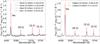 |
Fig. B.1 Comparison of the nebular lines in apertures located at 2.1″ in the North, South, East, and West of the star (left), and between the apertures with the highest and the lowest [S II]/Hα ratio (right). |
Appendix C Spectroscopic analysis of the B-star near [W60] B90
Apart from the long-slit spectroscopy observations presented in Table 1, we placed the slit in another position that was finally excluded from the analysis of [W60] B90 and the shocked material. The slit was centered at the coordinates RA=05:24:18.38 Dec= −69:38:54.9 on the star with Gaia DR3 ID 4657970853790677248 (Fig. C.1). The data was obtained on the same night as Epoch4 and Neb6, under the same technical settings, and reduced following the procedure described in Sect 2.2.
We analyze the spectral region 3900 − 4800Å (see Fig. C.2) using the criteria of Walborn & Fitzpatrick (1990) to determine the spectral classification of the star. The absence of He II lines and the presence of He I lines indicate a B spectral type. More specifically, the absence of He II λ4686 suggests a type later than B0.7, while the absence of Si II lines λλ4128 − 4130 supports a type not later than B2. The weak presence of C III+O II blends λλ4070 and 4650 suggests a B1 spectral type. The main criterion for the luminosity classification in B1 stars is the weakness of Si III λ4552 compared to He I λ4387, which suggests a V luminosity class. This classification is also supported by the low intensity of the Si IV λ4089 line compared to He I lines λλ4026 and 4121, as well as the low ratio of Si IV λ4116/He I λ4121. We therefore report a B1V spectral classification for this star. Furthermore, the feature in the right wing of Hγ and the RV inconsistency in the He I λ6678 line hint at a low luminosity companion, but further investigation is needed to confirm it. Finally, we find a Plmc=0.99 (see Sect. 3.1; Jiménez-Arranz et al. 2023) and a RV of 266 ± 7 km s−1 from the Balmer series, therefore confirming its membership to the LMC.
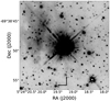 |
Fig. C.1 HST F675W image showing the location of [W60] B90 and the B-star, marked with a star symbol. |
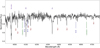 |
Fig. C.2 Spectral region showing the lines used to determine the B1V spectral type of the star. |
Appendix D Disentangling the origin of the nebular emission
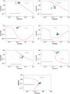 |
Fig. D.1 Diagnostic plots comparing the line ratio measurements (blue dots) in the CSM around [W60] B90 with the theoretical predictions of shocked vs. photoionized emission (red line, Kopsacheili et al. 2020). |
References
- Adams, S. M., Kochanek, C. S., Gerke, J. R., et al. 2017, MNRAS, 468, 4968 [Google Scholar]
- Alcock, C., Allsman, R. A., Alves, D., et al. 1997, ApJ, 486, 697 [NASA ADS] [CrossRef] [Google Scholar]
- Alcock, C., Allsman, R. A., Alves, D. R., et al. 1999, PASP, 111, 1539 [NASA ADS] [CrossRef] [Google Scholar]
- Antoniadis, K., Bonanos, A. Z., de Wit, S., et al. 2024, A&A, 686, A88 [NASA ADS] [CrossRef] [EDP Sciences] [Google Scholar]
- Anugu, N., Baron, F., Gies, D. R., et al. 2023, AJ, 166, 78 [NASA ADS] [CrossRef] [Google Scholar]
- Astropy Collaboration (Robitaille, T. P., et al.) 2013, A&A, 558, A33 [NASA ADS] [CrossRef] [EDP Sciences] [Google Scholar]
- Astropy Collaboration (Price-Whelan, A. M., et al.) 2018, AJ, 156, 123 [Google Scholar]
- Beasor, E. R., Davies, B., Smith, N., et al. 2020, MNRAS, 492, 5994 [Google Scholar]
- Bergemann, M., Kudritzki, R.-P., Plez, B., et al. 2012, ApJ, 751, 156 [Google Scholar]
- Bergemann, M., Kudritzki, R.-P., Würl, M., et al. 2013, ApJ, 764, 115 [NASA ADS] [CrossRef] [Google Scholar]
- Bergemann, M., Kudritzki, R.-P., Gazak, Z., et al. 2015, ApJ, 804, 113 [NASA ADS] [CrossRef] [Google Scholar]
- Bonanos, A. Z., Tramper, F., de Wit, S., et al. 2024, A&A, 686, A77 [NASA ADS] [CrossRef] [EDP Sciences] [Google Scholar]
- Chatys, F. W., Bedding, T. R., Murphy, S. J., et al. 2019, MNRAS, 487, 4832 [CrossRef] [Google Scholar]
- Choi, J., Dotter, A., Conroy, C., et al. 2016, ApJ, 823, 102 [Google Scholar]
- Cox, N. L. J., Kerschbaum, F., van Marle, A. J., et al. 2012, A&A, 537, A35 [NASA ADS] [CrossRef] [EDP Sciences] [Google Scholar]
- Cutri, R. M., Wright, E. L., Conrow, T., et al. 2021, VizieR Online Data Catalog: II/328 [Google Scholar]
- Davies, B., & Plez, B. 2021, MNRAS, 508, 5757 [NASA ADS] [CrossRef] [Google Scholar]
- Davies, B., Kudritzki, R.-P., Plez, B., et al. 2013, ApJ, 767, 3 [Google Scholar]
- Davies, B., Kudritzki, R.-P., Gazak, Z., et al. 2015, ApJ, 806, 21 [NASA ADS] [CrossRef] [Google Scholar]
- Davies, B., Crowther, P. A., & Beasor, E. R. 2018, MNRAS, 478, 3138 [NASA ADS] [CrossRef] [Google Scholar]
- Decin, L., Hony, S., de Koter, A., et al. 2006, A&A, 456, 549 [NASA ADS] [CrossRef] [EDP Sciences] [Google Scholar]
- Decin, L., Cox, N. L. J., Royer, P., et al. 2012, A&A, 548, A113 [Google Scholar]
- de Jager, C., Nieuwenhuijzen, H., & van der Hucht, K. A. 1988, A&AS, 72, 259 [NASA ADS] [Google Scholar]
- de Wit, S., Bonanos, A. Z., Tramper, F., et al. 2023, A&A, 669, A86 [NASA ADS] [CrossRef] [EDP Sciences] [Google Scholar]
- de Wit, S., Bonanos, A. Z., Antoniadis, K., et al. 2024, A&A, 689, A46 [NASA ADS] [CrossRef] [EDP Sciences] [Google Scholar]
- Dorda, R., & Patrick, L. R. 2021, MNRAS, 502, 4890 [NASA ADS] [CrossRef] [Google Scholar]
- Dorda, R., Negueruela, I., González-Fernández, C., & Tabernero, H. M. 2016, A&A, 592, A16 [NASA ADS] [CrossRef] [EDP Sciences] [Google Scholar]
- Dotter, A. 2016, ApJS, 222, 8 [Google Scholar]
- Drevon, J., Millour, F., Cruzalèbes, P., et al. 2024, MNRAS, 527, L88 [Google Scholar]
- Dupree, A. K., Strassmeier, K. G., Matthews, L. D., et al. 2020, ApJ, 899, 68 [Google Scholar]
- Dupree, A. K., Strassmeier, K. G., Calderwood, T., et al. 2022, ApJ, 936, 18 [NASA ADS] [CrossRef] [Google Scholar]
- Ekström, S., Georgy, C., Eggenberger, P., et al. 2012, A&A, 537, A146 [Google Scholar]
- Fraser, O. J., Hawley, S. L., & Cook, K. H. 2008, AJ, 136, 1242 [Google Scholar]
- Gaia Collaboration (Prusti, T., et al.) 2016, A&A, 595, A1 [NASA ADS] [CrossRef] [EDP Sciences] [Google Scholar]
- Gaia Collaboration (Vallenari, A., et al.) 2023, A&A, 674, A1 [NASA ADS] [CrossRef] [EDP Sciences] [Google Scholar]
- González-Torà, G., Wittkowski, M., Davies, B., & Plez, B. 2024, A&A, 683, A19 [NASA ADS] [CrossRef] [EDP Sciences] [Google Scholar]
- Gordon, K. D., Clayton, G. C., Misselt, K. A., Landolt, A. U., & Wolff, M. J. 2003, ApJ, 594, 279 [NASA ADS] [CrossRef] [Google Scholar]
- Groenewegen, M. A. T., & Sloan, G. C. 2018, A&A, 609, A114 [NASA ADS] [CrossRef] [EDP Sciences] [Google Scholar]
- Groenewegen, M. A. T., Sloan, G. C., Soszyński, I., & Petersen, E. A. 2009, A&A, 506, 1277 [NASA ADS] [CrossRef] [EDP Sciences] [Google Scholar]
- Guinan, E. F., Wasatonic, R. J., & Calderwood, T. J. 2019, ATel, 13341 [Google Scholar]
- Gvaramadze, V. V., Menten, K. M., Kniazev, A. Y., et al. 2014, MNRAS, 437, 843 [Google Scholar]
- Harper, G. M., Brown, A., & Guinan, E. F. 2008, AJ, 135, 1430 [Google Scholar]
- Harper, G. M., Brown, A., Guinan, E. F., et al. 2017, AJ, 154, 11 [Google Scholar]
- Henize, K. G. 1956, ApJS, 2, 315 [CrossRef] [Google Scholar]
- Heinze, A. N., Tonry, J. L., Denneau, L., et al. 2018, AJ, 156, 241 [Google Scholar]
- Hollis, J. M., Oliversen, R. J., Wagner, R. M., & Feibelman, W. A. 1992, ApJ, 393, 217 [NASA ADS] [CrossRef] [Google Scholar]
- Houck, J. R., Roellig, T. L., Van Cleve, J., et al. 2004, SPIE Conf. Ser., 5487, 62 [NASA ADS] [Google Scholar]
- Humphreys, R. M., & Jones, T. J. 2022, AJ, 163, 103 [NASA ADS] [CrossRef] [Google Scholar]
- Humphreys, R. M., Davidson, K., Ruch, G., & Wallerstein, G. 2005, AJ, 129, 492 [NASA ADS] [CrossRef] [Google Scholar]
- Humphreys, R. M., Helton, L. A., & Jones, T. J. 2007, AJ, 133, 2716 [NASA ADS] [CrossRef] [Google Scholar]
- Humphreys, R. M., Helmel, G., Jones, T. J., & Gordon, M. S. 2020, AJ, 160, 145 [NASA ADS] [CrossRef] [Google Scholar]
- Humphreys, R. M., Davidson, K., Richards, A. M. S., et al. 2021, AJ, 161, 98 [NASA ADS] [CrossRef] [Google Scholar]
- Humphreys, R. M., Richards, A. M. S., Davidson, K., et al. 2024, AJ, 167, 94 [NASA ADS] [CrossRef] [Google Scholar]
- Jayasinghe, T., Kochanek, C. S., Stanek, K. Z., et al. 2018, MNRAS, 477, 3145 [Google Scholar]
- Jiménez-Arranz, Ó., Romero-Gómez, M., Luri, X., et al. 2023, A&A, 669, A91 [NASA ADS] [CrossRef] [EDP Sciences] [Google Scholar]
- Jones, T. J., Shenoy, D., & Humphreys, R. 2023, Res. Notes Am. Astron. Soc., 7, 92 [Google Scholar]
- Josselin, E., & Plez, B. 2007, A&A, 469, 671 [NASA ADS] [CrossRef] [EDP Sciences] [Google Scholar]
- Joyce, M., Leung, S.-C., Molnár, L., et al. 2020, ApJ, 902, 63 [Google Scholar]
- Kaper, L., van Loon, J. T., Augusteijn, T., et al. 1997, ApJ, 475, L37 [NASA ADS] [CrossRef] [Google Scholar]
- Kelson, D. D. 2003, PASP, 115, 688 [NASA ADS] [CrossRef] [Google Scholar]
- Kelson, D. D., Illingworth, G. D., van Dokkum, P. G., & Franx, M. 2000, ApJ, 531, 159 [NASA ADS] [CrossRef] [Google Scholar]
- Kiss, L. L., Szabó, G. M., & Bedding, T. R. 2006, MNRAS, 372, 1721 [Google Scholar]
- Kochanek, C. S., Shappee, B. J., Stanek, K. Z., et al. 2017, PASP, 129, 104502 [Google Scholar]
- Kopsacheili, M., Zezas, A., & Leonidaki, I. 2020, MNRAS, 491, 889 [CrossRef] [Google Scholar]
- Kravchenko, K., Chiavassa, A., Van Eck, S., et al. 2019, A&A, 632, A28 [NASA ADS] [CrossRef] [EDP Sciences] [Google Scholar]
- Kravchenko, K., Jorissen, A., Van Eck, S., et al. 2021, A&A, 650, L17 [NASA ADS] [CrossRef] [EDP Sciences] [Google Scholar]
- Laplace, E., Götberg, Y., de Mink, S. E., Justham, S., & Farmer, R. 2020, A&A, 637, A6 [NASA ADS] [CrossRef] [EDP Sciences] [Google Scholar]
- Le Bertre, T., Matthews, L. D., Gérard, E., & Libert, Y. 2012, MNRAS, 422, 3433 [Google Scholar]
- Levesque, E. M. 2017, Astrophysics of Red Supergiants (Bristol, UK: IOP Publishing) [Google Scholar]
- Levesque, E. M., Massey, P., Olsen, K. A. G., et al. 2005, ApJ, 628, 973 [Google Scholar]
- Levesque, E. M., Massey, P., Olsen, K. A. G., & Plez, B. 2007, ApJ, 667, 202 [NASA ADS] [CrossRef] [Google Scholar]
- Levesque, E. M., Massey, P., Plez, B., & Olsen, K. A. G. 2009, AJ, 137, 4744 [NASA ADS] [CrossRef] [Google Scholar]
- Luridiana, V., Morisset, C., & Shaw, R. A. 2015, A&A, 573, A42 [NASA ADS] [CrossRef] [EDP Sciences] [Google Scholar]
- Ma, J.-Z., Chiavassa, A., de Mink, S. E., et al. 2024, ApJ, 962, L36 [NASA ADS] [CrossRef] [Google Scholar]
- Mackey, J., Mohamed, S., Neilson, H. R., Langer, N., & Meyer, D. M. A. 2012, ApJ, 751, L10 [NASA ADS] [CrossRef] [Google Scholar]
- MacLeod, M., Antoni, A., Huang, C. D., et al. 2023, ApJ, 956, 27 [CrossRef] [Google Scholar]
- Mainzer, A., Bauer, J., Grav, T., et al. 2011, ApJ, 731, 53 [Google Scholar]
- Mainzer, A., Bauer, J., Cutri, R. M., et al. 2014, ApJ, 792, 30 [Google Scholar]
- Marshall, J. L., Burles, S., Thompson, I. B., et al. 2008, SPIE, 7014, 701454 [Google Scholar]
- Mathewson, D. S., & Clarke, J. N. 1973, ApJ, 180, 725 [NASA ADS] [CrossRef] [Google Scholar]
- Meixner, M., Gordon, K. D., Indebetouw, R., et al. 2006, AJ, 132, 2268 [NASA ADS] [CrossRef] [Google Scholar]
- Meyer, D. M. A., Mignone, A., Petrov, M., et al. 2021, MNRAS, 506, 5170 [NASA ADS] [CrossRef] [Google Scholar]
- Mohamed, S., Mackey, J., & Langer, N. 2012, A&A, 541, A1 [Google Scholar]
- Montargès, M., Cannon, E., Lagadec, E., et al. 2021, Nature, 594, 365 [Google Scholar]
- Noriega-Crespo, A., van Buren, D., Cao, Y., & Dgani, R. 1997a, AJ, 114, 837 [NASA ADS] [CrossRef] [Google Scholar]
- Noriega-Crespo, A., van Buren, D., & Dgani, R. 1997b, AJ, 113, 780 [NASA ADS] [CrossRef] [Google Scholar]
- Osterbrock, D. E. 1989, Astrophysics of gaseous nebulae and active galactic nuclei (USA: University Science Books) [Google Scholar]
- Patrick, L. R. 2020, in XIV.0 Scientific Meeting (virtual) of the Spanish Astronomical Society, 174 [Google Scholar]
- Patrick, L. R., Evans, C. J., Davies, B., et al. 2017, MNRAS, 468, 492 [NASA ADS] [CrossRef] [Google Scholar]
- Patrick, L. R., Thilker, D., Lennon, D. J., et al. 2022, MNRAS, 513, 5847 [Google Scholar]
- Pietrzyński, G., Graczyk, D., Gallenne, A., et al. 2019, Nature, 567, 200 [Google Scholar]
- Pojmanski, G. 1997, Acta Astron., 47, 467 [Google Scholar]
- Renzo, M., Zapartas, E., de Mink, S. E., et al. 2019, A&A, 624, A66 [NASA ADS] [CrossRef] [EDP Sciences] [Google Scholar]
- Richards, A. M. S., Yates, J. A., & Cohen, R. J. 1996, MNRAS, 282, 665 [NASA ADS] [Google Scholar]
- Riebel, D., Srinivasan, S., Sargent, B., & Meixner, M. 2012, ApJ, 753, 71 [NASA ADS] [CrossRef] [Google Scholar]
- Riebel, D., Boyer, M. L., Srinivasan, S., et al. 2015, ApJ, 807, 1 [NASA ADS] [CrossRef] [Google Scholar]
- Shappee, B. J., Prieto, J. L., Grupe, D., et al. 2014, ApJ, 788, 48 [Google Scholar]
- Shenoy, D., Humphreys, R. M., Jones, T. J., et al. 2016, AJ, 151, 51 [NASA ADS] [CrossRef] [Google Scholar]
- Shingles, L., Smith, K. W., Young, D. R., et al. 2021, Transient Name Server AstroNote, 7, 1 [NASA ADS] [Google Scholar]
- Smartt, S. J. 2009, ARA&A, 47, 63 [NASA ADS] [CrossRef] [Google Scholar]
- Smartt, S. J. 2015, PASA, 32, e016 [NASA ADS] [CrossRef] [Google Scholar]
- Smartt, S. J., Eldridge, J. J., Crockett, R. M., & Maund, J. R. 2009, MNRAS, 395, 1409 [CrossRef] [Google Scholar]
- Stoop, M., Kaper, L., de Koter, A., et al. 2023, A&A, 670, A108 [NASA ADS] [CrossRef] [EDP Sciences] [Google Scholar]
- Sukhbold, T., Ertl, T., Woosley, S. E., Brown, J. M., & Janka, H. T. 2016, ApJ, 821, 38 [NASA ADS] [CrossRef] [Google Scholar]
- Tabernero, H. M., Dorda, R., Negueruela, I., & González-Fernández, C. 2018, MNRAS, 476, 3106 [NASA ADS] [CrossRef] [Google Scholar]
- Tetzlaff, N., Neuhäuser, R., & Hohle, M. M. 2011, MNRAS, 410, 190 [Google Scholar]
- Tonry, J. L., Denneau, L., Heinze, A. N., et al. 2018, PASP, 130, 064505 [Google Scholar]
- Udalski, A., Kubiak, M., & Szymanski, M. 1997, Acta Astron., 47, 319 [NASA ADS] [Google Scholar]
- Udalski, A., Soszynski, I., Szymanski, M. K., et al. 2008, Acta Astron., 58, 89 [NASA ADS] [Google Scholar]
- Udalski, A., Szymański, M. K., & Szymański, G. 2015, Acta Astron., 65, 1 [NASA ADS] [Google Scholar]
- Ulaczyk, K., Szymański, M. K., Udalski, A., et al. 2013, Acta Astron., 63, 159 [NASA ADS] [Google Scholar]
- van Loon, J. T., Cioni, M. R. L., Zijlstra, A. A., & Loup, C. 2005, A&A, 438, 273 [NASA ADS] [CrossRef] [EDP Sciences] [Google Scholar]
- Walborn, N. R., & Fitzpatrick, E. L. 1990, PASP, 102, 379 [Google Scholar]
- Watson, C. L., Henden, A. A., & Price, A. 2006, Soc. Astron. Sci. Ann. Symp., 25, 47 [NASA ADS] [Google Scholar]
- Wheeler, J. C., & Chatzopoulos, E. 2023, Astron. Geophys., 64, 3.11 [NASA ADS] [CrossRef] [Google Scholar]
- Wittkowski, M., Hauschildt, P. H., Arroyo-Torres, B., & Marcaide, J. M. 2012, A&A, 540, L12 [NASA ADS] [CrossRef] [EDP Sciences] [Google Scholar]
- Wright, E. L., Eisenhardt, P. R. M., Mainzer, A. K., et al. 2010, AJ, 140, 1868 [Google Scholar]
- Yang, M., & Jiang, B. W. 2011, ApJ, 727, 53 [NASA ADS] [CrossRef] [Google Scholar]
- Yang, M., Bonanos, A. Z., Jiang, B.-W., et al. 2018, A&A, 616, A175 [NASA ADS] [CrossRef] [EDP Sciences] [Google Scholar]
- Yang, M., Bonanos, A. Z., Jiang, B., et al. 2021, A&A, 646, A141 [EDP Sciences] [Google Scholar]
- Yang, M., Bonanos, A. Z., Jiang, B., et al. 2023, A&A, 676, A84 [NASA ADS] [CrossRef] [EDP Sciences] [Google Scholar]
Updated up to the submission date of the paper.
IRAF is distributed by the National Optical Astronomy Observatory, operated by the Association of Universities for Research in Astronomy (AURA) under agreement with the National Science Foundation.
All Tables
All Figures
|
Fig. 1 HST F675W image of [W60] B90 showing the PM analysis for PLMC = 0.7. The arrows represent the peculiar velocity direction of [W60] B90 for each cone to compute the local PM of the LMC. The length of the arrows is scaled with the peculiar velocity. The green dotted lines show the 1σ PM error from Gaia DR3 on the 4.5′ cone size. |
| In the text | |
|
Fig. 2 HST F675W image with the slits and the [S II]/Hα ratio for each aperture overlaid. The green color corresponds to ratios above 0.4 within the error, the yellow color corresponds to ratios with a lower limit below 0.4, and the red color corresponds to apertures below 0.4 within the error. |
| In the text | |
|
Fig. 3 Light curve of [W60] B90 indicating the respective survey and filter. Top: magnitudes obtained from each survey. Bottom: relative magnitude after subtracting the mean value of each data set. The vertical lines represent the epoch-spectroscopy as labeled in Table 1. |
| In the text | |
|
Fig. 4 Zoom in on the dimming events of [W60] B90. The first three panels show the comparison of the three dimmings of [W60] B90 with the Great Dimming of Betelgeuse (gray), the dimming of RW Cep (magenta), and a minimum from μ Cep (blue) in the V-band from AAVSO. The right panel overplots the photometry of the three dimmings of [W60] B90. We used the minimum of each data set as the zero-point reference for each graph. |
| In the text | |
|
Fig. 5 Mid-infrared light curve of [W60] B90 from NEOWISE and Spitzer. W1 and [3.6] are shown with full and open blue circles, respectively; W2 and [4.5] are shown with full and open green squares. ASAS-SN data are shown in gray with an offset for comparison. |
| In the text | |
|
Fig. 6 Comparison of the spectroscopic epochs of W60 [B90] in the optical (top) and the main TiO bands at 6150 and 7050 Å (bottom). The inset shows the light curve (as in Fig. 3) indicating each spectroscopic epoch with the dashed lines, following the color code of the spectra. |
| In the text | |
|
Fig. 7 Best MARCS model fit (red) for each epoch from MagE (black). Shaded areas in Epoch 1 show the spectral regions used in the fitting. |
| In the text | |
|
Fig. 8 Comparison between the best composite model (red), with 60% of the flux from a single Teff1 = 3950 K and 40% from Teff2 = 3300 K, and the best single model (gray) from Fig. 7 for Epoch 2. |
| In the text | |
|
Fig. 9 Derived parameters from the FIRE spectrum. Top: best fit of the FIRE spectrum (solid black) in the J-band for the LTE MARCS models (dashed-dot red) and the NLTE-corrected version (solid blue) with the NLTE effects applied to the indicated lines. The spectral regions used in the fitting are shown with gray shades. Bottom: best LTE MARCS model (dotted red) from the J-band to the FIRE spectrum (black). The model was reddened with E(B − V) = 1.05 mag to match the SED. The green-shaded region highlights the spectral region shown in the upper plot. |
| In the text | |
|
Fig. 10 SED of [W60] B90. The orange diamonds show the observations and the black line is the best-fit model from DUSTY, which is a superposition of attenuated flux (dashed light blue), the scattered flux (dot-dashed gray), and dust emission (dotted brown). The green curve represents the Spitzer IRS spectrum. |
| In the text | |
|
Fig. 11 Location of [W60] B90 (red triangle) in the Hertzsprung-Russell diagram of the RSG population in the LMC (black dots, Yang et al. 2021). The color map represents the central 12C mass fraction on the MIST evolutionary track, while the nodes indicate a step of 104 yr. |
| In the text | |
|
Fig. B.1 Comparison of the nebular lines in apertures located at 2.1″ in the North, South, East, and West of the star (left), and between the apertures with the highest and the lowest [S II]/Hα ratio (right). |
| In the text | |
|
Fig. C.1 HST F675W image showing the location of [W60] B90 and the B-star, marked with a star symbol. |
| In the text | |
|
Fig. C.2 Spectral region showing the lines used to determine the B1V spectral type of the star. |
| In the text | |
|
Fig. D.1 Diagnostic plots comparing the line ratio measurements (blue dots) in the CSM around [W60] B90 with the theoretical predictions of shocked vs. photoionized emission (red line, Kopsacheili et al. 2020). |
| In the text | |
Current usage metrics show cumulative count of Article Views (full-text article views including HTML views, PDF and ePub downloads, according to the available data) and Abstracts Views on Vision4Press platform.
Data correspond to usage on the plateform after 2015. The current usage metrics is available 48-96 hours after online publication and is updated daily on week days.
Initial download of the metrics may take a while.