| Issue |
A&A
Volume 690, October 2024
|
|
|---|---|---|
| Article Number | A242 | |
| Number of page(s) | 12 | |
| Section | The Sun and the Heliosphere | |
| DOI | https://doi.org/10.1051/0004-6361/202450343 | |
| Published online | 15 October 2024 | |
Coronal magnetic field and emission properties of small-scale bright and faint loops in the quiet Sun
1
Max Planck Institute for Solar System Research, Justus-von-Liebig-Weg 3, 37077 Göttingen, Germany
2
Space Research and Technology Institute, Bulgarian Academy of Sciences, Acad. Georgy Bonchev Str., Bl. 1, 1113 Sofia, Bulgaria
3
LESIA, Observatoire de Paris, Université PSL, CNRS, Sorbonne Université, Université Paris Cité, 5 place Jules Janssen, 92195, Meudon, France; Laboratoire Cogitamus, F-75005 Paris, France
4
School of Mathematics and Statistics, University of St Andrews, North Haugh, St Andrews, KY16 9SS Scotland, UK
Received:
12
April
2024
Accepted:
10
July
2024
Context. The present study provides statistical information on the coronal magnetic field and intensity properties of small-scale bright and faint loops in the quiet Sun.
Aims. We aim to quantitatively investigate the morphological and topological properties of the coronal magnetic field in bright and faint small-scale loops, with the former known as coronal bright points (CBPs).
Methods. We analyse 126 small-scale loops of all sizes using quasi-temporal imaging and line-of-sight magnetic field observations. These observations are taken by the Atmospheric Imaging Assembly (AIA) in the Fe XII 193 Å channel and the Helioseismic Magnetic Imager (HMI) on board the Solar Dynamics Observatory. We employ a recently developed automatic tool that uses a linear magneto-hydro-static (LMHS) model to compute the magnetic field in the solar atmosphere and automatically match individual magnetic field lines with small-scale loops.
Results. For most of the loops, we automatically obtain an excellent agreement of the magnetic field lines from the LMHS model and the loops seen in the AIA 193 Å channel. One stand-out result is that the magnetic field is non-potential. We obtain the typical ranges of loop heights, lengths, intensities, mean magnetic field strength along the loops and at loop tops, and magnetic field strength at loop footpoints. We investigate the relationship between all those parameters. We find that loops below the classic chromospheric height of 1.5 Mm are flatter, suggesting that non-magnetic forces (one of which is the plasma pressure) play an important role below this height. We find a strong correlation (Pearson coefficient of 0.9) between loop heights and lengths. An anti-correlation is found between the magnetic field strength at loop tops and loop heights and lengths. The average intensity along the loops correlates stronger with the average magnetic field along the loops than with the field strength at loop tops.
Conclusions. The latter correlation indicates that the energy release in the loops is more likely linked to the average magnetic field along the loops than the field strength on the loop tops. In other words, the energy is probably released all along the loops, but not just at the loop top. This result is consistent with a recent benchmarking radiative 3D MHD model.
Key words: Sun: atmosphere / Sun: chromosphere / Sun: corona / Sun: fundamental parameters / Sun: magnetic fields
© The Authors 2024
 Open Access article, published by EDP Sciences, under the terms of the Creative Commons Attribution License (https://creativecommons.org/licenses/by/4.0), which permits unrestricted use, distribution, and reproduction in any medium, provided the original work is properly cited.
This article is published in open access under the Subscribe to Open model.
Open Access funding provided by Max Planck Society.
1. Introduction
Coronal loops at all scales are the solar phenomena that dominate the solar corona when observed in extreme ultraviolet (EUV) emission from plasma heated to a million degrees. Loops in active regions (ARs) have been very intensively studied, and to a large extent, their morphological, magnetic, and plasma properties are well known (Reale 2014, and references therein). Bright small-scale loops in the quiet Sun, known as Coronal Bright Points (CBPs), were also studied in some details (for review see Madjarska 2019) although spatial and time resolution limitations have restricted certain investigations. Outside small- and large-scale loop regions, that is CBPs, and within ARs, the solar corona is filled with diffuse emission. Tiwari et al. (2023) suggested that most of the AR heating to high temperature is transient, while the background emission in ARs results from small, steady heating. Klimchuk & Porter (1995) proposed that the diffused quiet Sun emission component consists of fainter and less clearly distinguishable loops. Madjarska et al. (2023) demonstrated that this interpretation is indeed highly probable after deriving the properties of seven faint loops. The morphology and physical properties of CBP individual loops have received less attention. One reason is that before the TRansition Region and Coronal Explorer (TRACE), the Solar Dynamics Observatory (SDO), and the IRIS space missions, the limited spatial resolution of the existing instruments did not permit resolving individual loops. Hereafter, we will review some of the known properties of CBPs and their coronal magnetic structure.
The global sizes of CBPs have been typically determined by the diameter of their on-disc projected areas, assuming a circular shape. This approach was introduced at the time of the CBP discovery in 1969 (Vaiana et al. 1973) as they appeared in the limited-resolution of the first X-ray images as compact circle-like areas of enhanced emission with a diameter ranging from 20″ to 30″ (Golub et al. 1977). Although several studies also report on the size of CBPs, all of them use the same approach and found similar sizes (for more details see Section 3.4 in Madjarska 2019).
The heights of CBP loops, observed in extreme ultraviolet (EUV), mainly at coronal temperatures, have been estimated to range from 5 to 10 Mm with an average height of 6.5 Mm. Various methods have been employed; details can be found in section 3.5 of Madjarska (2019). To determine the heights of CBP loops in various temperatures, only CBPs nearby ARs have been studied as they are typically larger. Loops in emission from spectral lines with high formation temperatures were found to overlay cooler once. The CBP heights in chromospheric and transition region temperatures are estimated to extend to heights of 3 Mm (with 50% errors of this estimation).
The coronal magnetic topology of CBPs is crucial in modelling these phenomena. It was first derived by Parnell et al. (1994) and Mandrini et al. (1996). Pérez-Suárez et al. (2008) obtained the 3D structure of a CBP observed with several instruments on board TRACE, Solar Heliospheric Observatory (SoHO), and Hinode employing the Mpole code of Longcope (1996). From the visual comparison of the appearance of the CBP in enhanced Hinode’s X-ray Telescope (XRT) images and the extrapolated magnetic field (based on SoHO’s Michelson Doppler Imager magnetograms), Pérez-Suárez et al. (2008) concluded that a significant fraction of the magnetic field that builds up the skeleton of the CBP is close to potential. The loop lengths were reported in two studies. Mondal et al. (2023) employed a potential field model for a single CBP, and from all computed field lines, they estimated that lengths are in the range from a few megameters to up to 80 Mm, with a distribution that peaks at 30 Mm. Gao et al. (2022) also report the lengths of CBP loops obtained as L = πD/2, where D is the distance of the two footpoints of a loop. The authors find a 14–42 Mm length range, with an average of 23.5 Mm.
To the best of our knowledge, the coronal magnetic properties of small-scale loops in the quiet Sun and coronal holes have been investigated in a relatively small number of studies. Wiegelmann et al. (2010) used data from Sunrise/IMaX (Martínez Pillet et al. 2011). The study performed potential field extrapolations (linear force-free extrapolation was also tested). The force-free extrapolation was justified by the study of Martínez González et al. (2010), which noted that the loop topology appears potential as the magnetic fields at the footpoints become almost vertical when the loop crosses the minimum temperature region. Wiegelmann et al. (2010) investigated all magnetic loops that connect photospheric fluxes and found an average loop height of 1.24 ± 2.45 Mm with the magnetic field strength in the two footpoints of loops showing large differences.
Generally, there has been no attempt to estimate the length and heights of small-scale loops by directly matching individual loops with model-produced magnetic field lines. Although high-resolution images have existed since the time of the TRACE mission, more attention has been paid to AR loops, and attempts were made to find a methodology which can be used to extract the coronal magnetic properties of loops (Carcedo et al. 2003).
The main goal of the present study is to provide statistical information about the magnetic and morphological properties of small-scale loops, including their length, height, and magnetic field along the loops. The magnetic field observations are taken by the Helioseismic Magnetic Imager (HMI, Scherrer et al. 2012) and the imaging data by the Atmospheric Imaging Assembly (AIA, Lemen et al. 2012) on board SDO (Pesnell et al. 2012). The enumeration of the loop systems is identical to those in Paper I.
The paper is organized as follows: In Section 2, we briefly describe the data. Full details on the data are given in Paper I. Section 3 describes, in short, the methodology for computing linear magneto-hydro-static (LMHS) equilibria. Section 4 presents the results and discussion, including presentation and discussion on the obtained LMHS parameters (Section 4.2), the loop physical parameters (Section 4.3), and their relationship (Section 4.4). Section 5 gives a summary and the conclusions.
2. Observational data
The observations are described in full detail in (Madjarska et al. 2023, hereafter Paper I). Here, we summarize the main details of these data. We utilised imaging data from AIA (Lemen et al. 2012) on board SDO (Pesnell et al. 2012) taken in the Fe XII 193 Å channel (hereafter AIA 193) and HMI/SDO line-of-sight magnetograms (Scherrer et al. 2012). The data were collected over a period of 48 h starting on 2019, September 15, at 00:00 UT. The AIA 193 data have a 12-s cadence and 0.6″ × 0.6″ pixel size. To increase the signal-to-noise ratio, we binned every three consecutive AIA 193 images. We used HMI line-of-sight magnetograms taken at a 45-s cadence. The HMI data originally have a 0.5″ × 0.5″ pixel size but were rescaled to the AIA pixel size of 0.6″ using the hmi_prep.pro procedure. To increase the signal-to-noise ratio, we binned eight consecutive magnetograms. All images were derotated to 00:00 UT on September 16, 2019. The final cadence of the images is approximately 6 min. The events selected for this study are taken from a square field-of-view that covers −400″ to 400″ from the disc centre (or 1334 × 1334 px2) (see Fig. 1 in Paper I). The enumeration of the CBPs in the present paper is the same as in Paper I, allowing the reader to identify each CBP location in Fig. 1 of Paper I. The bright and faint loop systems were visually selected. The selection approach is described in full detail in Section 3 of Paper I.
3. Methodology: MHS equilibria
The present study employs a recently developed automatic algorithm to compute LMHS equilibria and match obtained field lines with features with enhanced emission in the SDO/AIA 193 channel (Wiegelmann & Madjarska 2023, hereafter Paper II). In the following, we will briefly describe the algorithm. The code uses line-of-sight HMI magnetograms as the photospheric boundary condition. While the solar corona is assumed to be force-free due to the low plasma β, which is not the case in the lower solar atmosphere. In the photosphere and chromosphere, the Lorentz force remains finite and needs to be compensated in the magneto-hydro-static (MHS) approximation by the plasma pressure gradient force and the gravity force. The MHS equations are:


where B is the magnetic field, j the electric current density, μ0 the permeability of free space, p the plasma pressure, ρ the mass density, and Ψ the gravitational potential. Zhu et al. (2022) provide a review of how these equations can be solved in their generic nonlinear form. Computing nonlinear MHS requires accurate photospheric magnetic vector field measurements, which are not available in the quiet Sun regions and coronal holes due to instrumental limitations.
For the study of loops in the quiet Sun, only the longitudinal magnetic field component Bl is measured accurately. Since the analyzed data are close to the Sun disc centre ( field of view of 400″ × 400″, 1″ ∼ 720 km), we neglect the small projection angle and assume that the vertical magnetic field component Bz = Bl. We, therefore, solve the special class of LMHS equations derived by Low (1991) by assuming that the electric current density can be written in the form:

This LMHS equation has three free parameters α, a, and κ. The parameter α defines the strength of the field-aligned electric currents (like for a force-free field). The parameter a is a pure number which measures the strength of the horizontal currents, and 1/κ prescribes the scale height of these currents. We compute the solution with the help of a Fast Fourier Transform (FFT). This technique was previously used to model magnetic structures where the plasma pressure and gravity deform the magnetic field, such as within filaments (Aulanier et al. 1999), in surges and arch filament systems (Mandrini et al. 2002). For the required flux balance in the FFT method, we compute mirror magnetograms as introduced by Seehafer (1978). The original magnetogram, in the range x = 0…Lx, y = 0…Ly, is mirrored to the regions with x < 0 or/and y < 0 to fill the region x = −Lx…Lx, y = −Ly…Ly. The mirroring assumed that Bz(−x, y, 0) = − Bz(x, y, 0), Bz(x, −y, 0) = − Bz(x, y, 0), and Bz(−x, −y, 0) = Bz(x, y, 0) (where x > 0, y > 0). Then, the final magnetogram, twice larger in x and y directions, is flux-balanced by construction.
The FFT method solves the LMHS for given free parameters α, a, and κ. These three parameters are apriori unknown and need to be computed from additional observations, here coronal images. To do so, we apply the recently developed algorithm to compute the optimum LMHS parameters by comparing closed magnetic field lines with plasma loops as seen in EUV images. The main idea of this approach is to compare closed magnetic field lines (which are an output of the MHS code with arbitrary parameters) with the emissivity seen in coronal images (see Paper II for details).
Our method is a generalization of a method developed by Green (2002), then by Carcedo et al. (2003), where the optimum linear force-free parameter α was computed by scanning the whole parameter space and field lines were computed from footpoints limited to a manually selected area. Here, our approach rather selects the footpoint areas automatically and chooses, as a standard option, the strongest positive and negative magnetic elements from the magnetogram. All field lines connecting these footpoint areas are projected onto the EUV image. Then, for each field line, we apply the following procedure: We extract the EUV emissivity from AIA data along the magnetic field line on a band of ±3 pixels perpendicular to it. The lateral extension is limited to minimise the inclusion of emission other than the EUV loop emission which will be selected during the minimisation process. In the frame of the field line curvilinear abscissa and its orthogonal direction, the emissivity is located within an elongated rectangle with the selected field line located by definition along the central axis (as shown in Fig. 1). At each location, j ( = 0 to m − 1) along the field line, the emissivity in the perpendicular direction is fitted with a Gaussian function. The shift of the Gaussian called Nmax provides a measure of the distance between the field line and the fitted EUV loop. How well the full field line agrees with the loop in EUV is quantified with
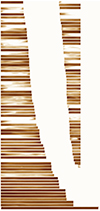 |
Fig. 1. All 126 examples of the uncurled loops.The colour level shows the AIA 193 intensity on a linear scale. The loops are arranged by the loop length. |
The quantity Ci2 has to be minimized over all the computed field lines with respect to the model parameters as

This defines α, a, and κ for the studied region containing the loop, as well as the field line which best matches the EUV loop. Finally, the method creates a so-called uncurled EUV image when convergence is achieved. Examples are shown in Fig. 1.
A further sophistication is that in images with several close-by EUV loops, we aim to select the brightest loop. This is done by defining

where Iuncurled is the observed loop intensity, integrated along and across the uncurled loop and normalized to the average emissivity of the image. In the present study, we choose n = 1. This functional LMHS has to be minimized to find the optimum model parameters α, a, κ, which is done with the help of a simplex-downhill method as defined in Wiegelmann & Madjarska (2023), Section 6 ‘fully automatic method’. To save computing time, we evaluated in this first step only magnetic field lines which magnetically connect the strongest positive and strongest negative magnetic elements in the FOV. We refer to it as the standard approach.
A visual inspection of the resulting magnetic loops revealed that, in several cases, the loops visible in the AIA 193 images did not connect the strongest negative and positive flux concentrations in the HMI image data. We recomputed these cases with other magnetic element pairs selected by hand. We refer to it as a non-standard approach. The photospheric magnetic field of the loops analysed here is far above the HMI errors of 10 G and, in the present case, 4 G, as we used 8 binned magnetograms; therefore, the extrapolation accuracy is highly reliable.
4. Results and discussion
4.1. Global description
For this study, we randomly chose 189 frames containing small-scale loop systems (SSLSs), some bright, others faint, as selected in Paper II. The challenges of using all 189 frames come from the fact that not all loops can be fitted with the automatic algorithm, and finding the best parameters is time-consuming. Of those, in 126 frames, we found a good agreement between a magnetic field line and a coronal loop seen in AIA 193. In the first column of Table A.1, we list each SSLS as bpXXX, where XXX is the numeration as in Paper I, and eleven of these loops were extracted from faint SSLSs as noted in Paper I. We should remark that some of the other loops are also fainter, although they compose generally bright SSLSs, that is, CBPs. The procedure selects the brightest loop when several loops are in the same frame. Some of the 126 loops were selected in the same loop system to test the temporal variation of α, a, and κ as well as the topological and quantitative properties of different loops in the same SSLSs or the temporal changes of the same loop. Concerning the latter, a dedicated study is in progress using 45 sec cadence AIA and HMI data. These loops are often taken in consecutive or close-by-in-time images.
For 97 out of 126 loops (77%), the modelling is done with the standard approach, that is, the loops connect the strongest positive and strongest negative magnetic elements. The remaining 29 loops (23%) are obtained with a non-standard approach. This is noted in column 6 (named App) of Table A.1, where ‘St’ refers to parameters obtained with a standard approach and ‘NSt’ to those obtained with a non-standard approach. In Fig. 1, we present the uncurled loops of all successfully extrapolated loop examples (126) sorted by their lengths. It can be noted that longer loops tend to be fainter.
In Fig. 2, two examples of loops obtained with the fully automatic algorithm (standard) are shown, while Fig. 3 presents two examples of the non-standard approach. A 3D view of all four loops is presented in Fig. 4. The rest of the loop cases analysed here (as in the left panels in Figs. 2 and 3) are archived at Zenodo. Finally, the detailed results obtained for the 126 loops are given in Table A.1, including the parameters α, a and κ in columns 3, 4 and 5; the averaged intensity (I, column 7), the loop lengths (L, column 8), height (H, column 9), the magnetic flux in the positive and negative footpoints of the loop (Bpos and Bneg, columns 10 and 11) and the average magnetic flux along the loop (Bav, in column 12). In Paper I, we provide the animations (intensity and photospheric magnetic field evolution) of all SSLSs studied there1.
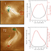 |
Fig. 2. Two examples of loops fitted with the fully (standard) automatic algorithm (cases 1 and 72). Left: AIA 193 intensity with the best field line (black line) fitted a loop. The circles mark the potential footpoint areas as automatically selected by the algorithm. Only closed magnetic field lines with footpoints in these circled areas are considered for the fitting procedure. The three black and green contours indicate negative polarities. The three orange and red contours outline positive polarities. All contours are relative to the absolute maximum field strength in the magnetograms, equispaced between 0 and max |Bz|. The intensity of each image is scaled to the maximum intensity of the image. Right: black curve shows the magnetic field strength along the loop length as obtained from the LMHS model. The red curve gives the loop height along its length. |
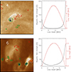 |
Fig. 3. Same as Fig. 2 of cases 4 and 6 for field lines obtained using a non-standard approach. See Section 4.1 for details. |
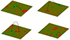 |
Fig. 4. Four examples of 3D loop views. The best-computed field lines are shown in black lines that match the observed AIA 193 loops. The observed magnetograms are shown at the bottom of the 3D plots with green/red colours for negative/positive Bz values, respectively. Top row: HMI magnetogram of cases 1 and 72 shown in Fig. 2. Bottom row: same for cases 4 and 6 shown in Fig. 3. |
4.2. LMHS parameters
In the second column of Table A.1, we provide the functional LMHS for all 126 loops. The smaller the value of LMHS in Eq. (7), the better the magnetic field lines and AIA 193 loops agree. For 94 out of the 126 loops, we get LMHS < 1 (see Paper II for more details about the functional LMHS). Visual inspection confirms the excellent agreement of the magnetic-field lines obtained from the LMHS modelling and the loops seen in the AIA 193 Å channel (log T ∼ 1 MK). The optimum solution is when LMHS is equal to zero (for more details, see Paper II). Higher values of LMHS correspond to worse agreement between a field line and a loop seen in AIA 193. The reason for that is that at some points along the field line, the maximum of the EUV emissivity is shifted away from the field lines, leading to higher values in Eq. (5), for example, cases 24 and 39. Higher values in LMHS can also occur for very faint plasma loops when Iuncurled in the functional of Eq. (7) becomes very small, such as cases 85 and 87.
As mentioned above, in columns 3–5 of Table A.1 annotated with α, a, and κ, we show the corresponding optimized parameters of the LMHS model as defined in Eq. (4). As mentioned in Section 3, the parameter α controls the field-aligned electric current density. The higher the absolute value of α, the stronger the electric current is. For positive values of α, the currents are parallel to the magnetic field and for negative values of α, the currents are antiparallel to the magnetic field. The parameter a controls the horizontal currents, which are partly perpendicular to the magnetic field lines and cause a finite Lorentz force. Large values of a mean that the magnetic structure is far away from a force-free equilibrium. Finally, κ defines how fast the non-magnetic forces decrease with height. If the parameter a = 0, we have no Lorentz force and the LMHS model reduces to a linear force-free model, which is the case for 14 cases.
A subclass of linear force-free equilibria are potential fields where also α = 0. This is not the case in any of the investigated examples, except for case 2, where α = 0.01 so that the magnetic field is nearly potential. The α values reported in Table A.1 are normalized by the magnetogram size. Out of all 126 loops, only 32 have a value of |α|< 1.0 and 17 of them have |α|< 0.5. These loops have rather moderate field-aligned electric currents, that is, the field is close to potential for these cases. All other force-free loops have absolute values of |α| up to 6 and contain rather strong field-aligned electric currents.
The parameter a is a dimensionless number in Eq. (4), which is limited in the model to a ≤ 1.2. Only 10 loops have a = 0. Moreover, only one loop (case 20) has both a = 0 and a small value of α = −0.14, which is very close to a potential magnetic field.
The ratio 1/κ is the height at which the non-magnetic forces drop to 1/e (about 37%). This can be assumed to be the height of the forced layer. In Table A.1 1/κ is given in Mm−1. For instance, for a pixel size of 432 km, as in the present work, the forced layer has a height of 2.2 Mm for κ = 0.2 and a height of 0.72 Mm for κ = 0.6. If a is equal to zero, we have a force-free field and, therefore, no κ. The values of 1/κ are typically small, and the median is only 0.7 Mm, so about half of the vertical extension of the classical chromosphere. The median of loop height is also small, 2.7 Mm, while still above a factor 3 larger than the median of 1/κ. This means that, apart from their footpoints, most loops have nearly a force-free field in the corona above the forced layer.
Cases 25 and 26 correspond to the same loop recorded 6 min apart. One could note that the parameter α has changed from −0.16 to 0.16 which can be considered negligible. The same is valid for all other parameters (see Table A.1). The same can be seen for cases 43 and 44, where the images are taken 12 min apart. Cases 110–115 sample different loops in the same CBP, BP046, with a time difference between the frames from 12 min to 14 h (the time difference between two frames is 6 min as explained in Paper I). The loops are found to have a different α parameter, ranging from −0.8 to 5.5 indicating the energetic complexity of small-scale systems as in ARs (e.g. Reale 2014).
We learned from the investigation in Paper II that α influences the loop-fitting more than a and κ. This is linked to the small vertical extension of the forced layer compared to the loop height (so a large fraction of loops are typically force-free). As tested in Paper II, it is possible to do a constraint optimization (fix a and κ) and vary only α. From the few examples in Paper II, the fitting (values of LMHS) is only slightly worse than fitting all three parameters. This could be further explored in the future if we have, for instance, vector magnetograms from which we could deduce a from measurements at photospheric and chromospheric heights (e.g. with photospheric and chromospheric vector magnetograms). Furthermore, we could compute the Lorentz force and the related parameter a in both photospheric and chromospheric magnetograms to find out how fast a drops with height from the photosphere.
4.3. Loop physical parameters
Table 1 summarizes some of the physical parameters obtained from the LMHS model. The loops’ height (H) range is from 0.2 Mm (we exclude here case 28, which has a height of 0.01 Mm) to 13 Mm. We find that 38 loops have heights below 1.5 Mm (the typical height of the chromosphere) and 88 loops above 1.5 Mm. The average height, taking into account all 126 loops, is 4 Mm. Loop lengths are in the range from 1.4 Mm to 60 Mm with a median of 15 Mm. The average loop length for loops below typical chromospheric heights of 1.5 Mm is 8 Mm, while above this height is 20 Mm. For comparison, loop heights measured in active regions are typically in the range of 10–93 Mm and have loop lengths in the range from 60 to 350 Mm (e.g. Aschwanden et al. 2008; Xie et al. 2017). Thus, the loops studied here are significantly shorter than AR loops.
Statistics of the morphological and magnetic properties of small-scale loops.
A natural question to address is whether the field lines with low heights, that is, as low as 0.2 Mm, indeed confine plasmas heated to a million degrees. As a matter of fact, the observations show very short, bright, elongated EUV features connecting magnetic flux concentrations of opposite polarities. Those short bright loops are typically observed towards the end of the lifetime of SSLSs (see the animation of Paper I). To further explore the truthfulness of this observation, that indeed small-low lying loops confining million-degree plasma exist, one can employ spectroscopic and imaging co-observations as done in section 4 of the study by Madjarska & Doyle (2008). Such data permit investigation of whether the emission in the imaging channels comes from plasma at transition region or even chromospheric temperatures rather than coronal. It is well known that coronal EUV imaging channels could be contaminated with such emission, including SDO/AIA 193 (for details see Mou et al. 2018; Tiwari et al. 2022 and references therein). A forthcoming study will employ data from the IRIS, SDO/AIA and Solar Orbiter Extreme-Ultraviolet Imager (EUI) to explore this in full detail.
The loops studied here have a median (average) length/height ratio of 9 (12) for the loops with heights below 1.5 Mm and 4 (5) for loops higher than 1.5 Mm. The median (average) length/height ratio for all 126 loops is 5 (7). This indicates that lower loops are significantly flatter than a half-circle loop (length/height =π), while higher loops are more rounded. The flatness of lower loops is due to the significant role of non-magnetic forces including gravity and plasma pressure at heights below 1.5 Mm (classical chromospheric top height).
The average magnetic field strength B along the loops when all loops are considered ranges from 5 G to 81 G. Loops with heights below 1.5 Mm reach maximum values of B of 66 G, while B can be as high as 81 G for loops higher than 1.5 Mm. However, if we consider the average values, they indicate that loops lower than 1.5 Mm have similar average magnetic-field strength along the loops than the higher loops (25 G compared to 23 G, respectively).
The average magnetic field B at loop tops for lower loops (< 1.5 Mm) is 17 G compared to 8 G for the higher loops (heights above 1.5 Mm), which is a factor 2 lower. These are mean tendencies within a broad range of values from 1 G to 60 G for all the loops. For lower loops (heights below 1.5 Mm), the maximum of B is twice higher (60 G) than for loops above 1.5 Mm (33 G), so the same result as above with the average magnetic field B at loop tops.
Next, we compared the footpoint magnetic field measure from the starting(end)-point to a field line. The magnetic field of the loop footpoints is from ∼500 G (max Bstrong) to as weak as ∼0.3 G (min Bweak). Lower loops are rooted in a weaker magnetic field with an average Bweak/Bstrong of 22/50, while for higher loops, the values are 58/138, that is twice higher. The difference in the magnetic field strength in the two footpoints may cause siphon flow (Bethge et al. 2012). However, to establish this, spectroscopic data are needed to obtain the Doppler velocities. This will be the subject of another future statistical work where Interface Region Imaging Spectrograph (IRIS) data will be employed.
The inclination of the magnetic field (defined as the angle between B and the vertical z-axis) was also explored. We find some correlation between the inclination at the weak and strong B footpoints with a Pearson correlation coefficient cP = 0.52 (Fig. B.3, left panel). The inclination in both footpoints anti-correlates with loop heights with the same Pearson coefficient cP = −0.47 (Fig. B.3, middle and right panels). Indeed, it is expected that higher loops have more vertical footpoints. Very weak anti-correlation is found for the strong (cP = −0.28) and weak (cP = −0.25) magnetic field footpoints and loop length.
4.4. Relationship of loop physical parameters
Figures B.1 and B.2 provide the statistical correlation for the various loop parameters. The highest correlation is between the lengths and heights of the loops with a Pearson correlation coefficient cP = 0.9, Fig. B.1a. We obtained a power law index γ = 1.46 for the linear fit log(H) = γ log(L)−1.3. One can notice that loops with lower heights deviate asymmetrically from the linear fit, possibly related to the influence of gravity and pressure at lower heights.
We found a relatively high correlation (cP = 0.6) between the magnetic field strength in the two footpoints (Fig. B.1b). The relationship is a power law of log(Bweak) = 0.85 log(Bstrong)−0.2. There is some, although not a strong correlation between the footpoints with stronger and weaker magnetic fields and loop heights (cP = 0.46 and 0.45, respectively, (Figs. B.1c, d). For the power law relationships, we obtained log(H) = 0.7 log(Bstrong)−0.9 and log(H) = 0.36 log(Bweak)−0.1, respectively. The correlation is weaker for the magnetic field at footpoints versus loop lengths, cP of 0.34 and 0.31, respectively (Figs. B.1e, f). The two relationships could be represented in average with the power laws of log(L) = 0.32 log(Bstrong)+0.5 and log(L) = 0.16 log(Bweak)+0.9, respectively.
Next, we describe the correlations between the magnetic field strength at the loop top and its mean along the loop. First, we notice that the loop with the smallest length and height is isolated from the other loops (Figs. B.2a, c, d). Therefore, we excluded it from our statistics. Next, there is a clear anti-correlation between the field strength on the loop tops (Btop) and heights (cP = −0.59, Fig. B.2a). The relationship is a power law of log(H) = − 0.89 log(Btop)+1.2. As in Fig. B.1a, the smaller loop heights (below ∼2 Mm) deviate asymmetrically from the linear fit in Fig. B.2a. A slightly stronger correlation is present with loop lengths (cP = −0.64, Fig. B.2c) and the power law relation is log(L) = − 0.59 log(Btop)+1.7. In contrast, we found a weak correlation between the average magnetic field strength along the loop Bav and the loop heights and lengths with cP = −0.3 and −0.44, Fig. B.2b and d, respectively. The two relationships are a power law of log(Bav) = − 0.63 log(H)+1.2 and log(Bav) = −0.62 log(L)+2.0, respectively.
This contrasts with the results of Mandrini et al. (2000) obtained for coronal loops within active regions (ARs) where cP = −0.88 between the loop Bav and lengths. However, this result is obtained in different conditions: within ARs, with 100 ≤ Bfoot ≤ 500 G and for longer loops (50 ≤ L ≤ 300 Mm). They found that for L below 50 Mm, Bav is almost independent of loop length in ARs. Here, a similar result is obtained in the quiet Sun.
Next, we investigated the correlation with the loop intensity, which is defined as an average along the loop length with 1 pixel on both sides of the loop centre. The lengths and heights of the loops are uncorrelated with the loop intensity (cP of −0.19 and −0.12, respectively). The intensity of the loop is correlated (cP = 0.58, log(I) = 0.74log(Bav)+1.2) with the average magnetic field strength along the loop (Fig. B.2f). This correlation is stronger than the intensity correlation with the field strength on the loop tops (cP = 0.35, Fig. B.2e). The relationship is a power law of log(I) = 0.28 log(Btop)+2.0. These correlations indicate that the energy release in the loop is more linked to the average B along the loop than the field strength on the loop top. In other words, the energy is likely released all along the loops, not only at the loop tops. This is plausible, but it remains that the short length of the loops allows for the efficient redistribution of the input energy along the loop. The thermal conduction could be so efficient in such short loops (it scales as L−2) that it could transfer the energy input all along the loop, independently of its original input location. In comparison to X-ray loops in ARs, the results show a dispersion that is broadly similar to the present result. In Figures 1 and 2 of Klimchuk & Porter (1995), the temperature and plasma pressure are anti-correlated with loop lengths but with a substantial dispersion. Mandrini et al. (1996) investigated the relationship between loop length and B but only statistically (not for individual loops). B was found to anti-correlate with loop lengths with also significant dispersion (Figure 2 in their paper). To conclude, we can speculate that the loop intensity, which is a function of plasma density and temperature, is correlated with B but with a substantial dispersion.
This brings us to the discussion and future applications of the present study for the validation of present and future models of small-scale loops that confine plasma heated to a million degrees. The most recent are the 3D radiative MHD models by Nóbrega-Siverio et al. (2023) and Chen et al. (2022). While the former is based on the Bifrost code (Gudiksen et al. 2011), the latter employs the MURaM code (Vögler et al. 2005; Rempel 2017). Previously, all CBP models were built on ad-hoc driving mechanisms, and magnetic reconnection was employed as the main heating mechanism. One pioneering model for its time is the so-called Converging Flux Model (CFM) (e.g. Priest et al. 1994; von Rekowski et al. 2006) where the magnetic energy is converted through magnetic reconnection in the corona to thermal energy. More recently, Wyper et al. (2018) developed a model exploring the formation of CBPs in coronal holes and associated collimated flows, that is, jets.
The model by Nóbrega-Siverio et al. (2023) has been specifically developed to understand the plasma heating of small-scale loops that are the subject of investigation in the present study. In this model, the energy injection is produced through surface convection. The model explains the sustainability of the CBP heating for several hours. It also provides unprecedented observational diagnostics compared with simultaneous space and ground observations. The model is based on fan-spine configuration and demonstrates how stochastic motions associated with photospheric convection can significantly stress the CBP magnetic field topology, leading to important Joule and viscous heating around the CBP inner spine at a few megameters above the solar surface (transition region and low corona). Magnetic reconnection in the null point in the corona has some but lesser (than the Joule and viscous) heating contribution. The results from the present study will be directly compared with this model to verify its validity and will be reported in a forthcoming study.
5. Summary and conclusions
We presented here the first-of-its-kind statistical study on the coronal magnetic field properties of small-scale loops observed in emission with formation temperatures at ∼1 MK. The brighter of these loops compose the so-called coronal bright points. The study employs a recently developed automatic algorithm to compute LMHS equilibria that match computed field lines with enhanced emission features in the SDO/AIA 193 channel.
We reported the statistical properties of 126 loops for which we found a good agreement between a computed magnetic field line and an observed coronal loop seen in the Fe XII 193 Å channel of AIA. The magnetic field is found to be non-potential, with rare cases of field lines that are close to potential. Loops preserve the same α for a short time period, which is at least 6 min. A forthcoming dedicated study will explore the lifetime and temporal variation of the coronal magnetic properties of small-scale loops using a 45 s data cadence.
We summarize here our main results. The average loop height is 4 Mm, while the average loop length is 17 Mm. Loops at lower heights, below 1.5 Mm (considered classic chromospheric height), are flatter, possibly caused by the role of gravity and plasma pressure that are in play at these heights. The average magnetic field strength B along the loops ranges from 5 G to 81 G. The magnetic field at loop tops varies from 1 G to 60 G. The highest Pearson correlation coefficient (cP) is found between the lengths and heights of the loops (cP = 0.9).
The loop intensity correlates stronger with the average magnetic field along the loops than with the magnetic field at loop tops, suggesting that the main energy deposition that causes the plasma to heat to up to a million degrees does not happen on loop tops but rather occurs at lower heights along the loops as also predicted by the recent model of Nóbrega-Siverio et al. (2023). Meanwhile, simulations with the MURaM code by Chen et al. (2022) have suggested magnetic braiding as a possible mechanism for the heating of small-scale loops without presenting a detailed investigation, which is hopefully forthcoming.
The present study will be extended to data from the Solar Orbiter EUI high-resolution imager. Given its higher spatial resolution, it is likely that one AIA 193 loop will be composed of several strands. Therefore, the properties of the loop may depend on the number of strands and their degree of interlacement. At the photospheric level, it will be worthwhile to determine if the magnetic field (B) is monolithic or consists of several flux concentrations.
Data availability
All loop extrapolation examples are available at https://zenodo.org/records/13229635
Acknowledgments
We want to thank very much the referee for their helpful comments and suggestions. MM and TW acknowledge DFG grants WI 3211/8-1 and WI 3211/8-2, project number 452856778. TW acknowledges DLR grant 50OC2301. The HMI and AIA data are provided by the NASA/SDO science teams and have been retrieved using Stanford University’s Joint Science Operations Centre/Science Data Processing Facility. MM and KG thank the ISSI (Bern) for supporting the team “Observation-Driven Modelling of Solar Phenomena.”
References
- Aschwanden, M. J., Wülser, J.-P., Nitta, N. V., & Lemen, J. R. 2008, ApJ, 679, 827 [NASA ADS] [CrossRef] [Google Scholar]
- Aulanier, G., Démoulin, P., Mein, N., et al. 1999, A&A, 342, 867 [NASA ADS] [Google Scholar]
- Bethge, C., Beck, C., Peter, H., & Lagg, A. 2012, A&A, 537, A130 [NASA ADS] [CrossRef] [EDP Sciences] [Google Scholar]
- Carcedo, L., Brown, D. S., Hood, A. W., Neukirch, T., & Wiegelmann, T. 2003, Sol. Phys., 218, 29 [NASA ADS] [CrossRef] [Google Scholar]
- Chen, F., Rempel, M., & Fan, Y. 2022, ApJ, 937, 91 [NASA ADS] [CrossRef] [Google Scholar]
- Gao, Y., Tian, H., Van Doorsselaere, T., & Chen, Y. 2022, ApJ, 930, 55 [NASA ADS] [CrossRef] [Google Scholar]
- Golub, L., Krieger, A. S., Harvey, J. W., & Vaiana, G. S. 1977, Sol. Phys., 53, 111 [NASA ADS] [CrossRef] [Google Scholar]
- Green, L. M., López fuentes, M. C., Mandrini, C. H., et al. 2002, Sol. Phys., 208, 43 [Google Scholar]
- Gudiksen, B. V., Carlsson, M., Hansteen, V. H., et al. 2011, A&A, 531, A154 [NASA ADS] [CrossRef] [EDP Sciences] [Google Scholar]
- Klimchuk, J. A., & Porter, L. J. 1995, Nature, 377, 131 [NASA ADS] [CrossRef] [Google Scholar]
- Lemen, J. R., Title, A. M., Akin, D. J., et al. 2012, Sol. Phys., 275, 17 [Google Scholar]
- Longcope, D. W. 1996, Sol. Phys., 169, 91 [NASA ADS] [CrossRef] [Google Scholar]
- Low, B. C. 1991, ApJ, 370, 427 [NASA ADS] [CrossRef] [Google Scholar]
- Madjarska, M. S. 2019, Liv. Rev. Sol. Phys., 16, 2 [Google Scholar]
- Madjarska, M. S., & Doyle, J. G. 2008, A&A, 482, 273 [NASA ADS] [CrossRef] [EDP Sciences] [Google Scholar]
- Madjarska, M. S., Galsgaard, K., & Wiegelmann, T. 2023, A&A, 678, A32 [NASA ADS] [CrossRef] [EDP Sciences] [Google Scholar]
- Mandrini, C. H., Démoulin, P., Van Driel-Gesztelyi, L., et al. 1996, Sol. Phys., 168, 115 [NASA ADS] [CrossRef] [Google Scholar]
- Mandrini, C. H., Démoulin, P., & Klimchuk, J. A. 2000, ApJ, 530, 999 [NASA ADS] [CrossRef] [Google Scholar]
- Mandrini, C. H., Démoulin, P., Schmieder, B., Deng, Y. Y., & Rudawy, P. 2002, A&A, 391, 317 [NASA ADS] [CrossRef] [EDP Sciences] [Google Scholar]
- Martínez González, M. J., Manso Sainz, R., Asensio Ramos, A., & Bellot Rubio, L. R. 2010, ApJ, 714, L94 [CrossRef] [Google Scholar]
- Martínez Pillet, V., del Toro Iniesta, J. C., Álvarez-Herrero, A., et al. 2011, Sol. Phys., 268, 57 [CrossRef] [Google Scholar]
- Mondal, B., Klimchuk, J. A., Vadawale, S. V., et al. 2023, ApJ, 945, 37 [NASA ADS] [CrossRef] [Google Scholar]
- Mou, C., Madjarska, M. S., Galsgaard, K., & Xia, L. 2018, A&A, 619, A55 [NASA ADS] [CrossRef] [EDP Sciences] [Google Scholar]
- Nóbrega-Siverio, D., Moreno-Insertis, F., Galsgaard, K., et al. 2023, ApJ, 958, L38 [CrossRef] [Google Scholar]
- Parnell, C. E., Priest, E. R., & Golub, L. 1994, Sol. Phys., 151, 57 [NASA ADS] [CrossRef] [Google Scholar]
- Pérez-Suárez, D., Maclean, R. C., Doyle, J. G., & Madjarska, M. S. 2008, A&A, 492, 575 [NASA ADS] [CrossRef] [EDP Sciences] [Google Scholar]
- Pesnell, W. D., Thompson, B. J., & Chamberlin, P. C. 2012, Sol. Phys., 275, 3 [Google Scholar]
- Priest, E. R., Parnell, C. E., & Martin, S. F. 1994, ApJ, 427, 459 [Google Scholar]
- Reale, F. 2014, Liv. Rev. Sol. Phys., 11, 4 [Google Scholar]
- Rempel, M. 2017, ApJ, 834, 10 [Google Scholar]
- Scherrer, P. H., Schou, J., Bush, R. I., et al. 2012, Sol. Phys., 275, 207 [Google Scholar]
- Seehafer, N. 1978, Sol. Phys., 58, 215 [NASA ADS] [CrossRef] [Google Scholar]
- Tiwari, S. K., Hansteen, V. H., De Pontieu, B., Panesar, N. K., & Berghmans, D. 2022, ApJ, 929, 103 [NASA ADS] [CrossRef] [Google Scholar]
- Tiwari, S. K., Wilkerson, L. A., Panesar, N. K., Moore, R. L., & Winebarger, A. R. 2023, ApJ, 942, 2 [NASA ADS] [CrossRef] [Google Scholar]
- Vaiana, G. S., Krieger, A. S., & Timothy, A. F. 1973, Sol. Phys., 32, 81 [NASA ADS] [CrossRef] [Google Scholar]
- Vögler, A., Shelyag, S., Schüssler, M., et al. 2005, A&A, 429, 335 [Google Scholar]
- von Rekowski, B., Parnell, C. E., & Priest, E. R. 2006, MNRAS, 369, 43 [NASA ADS] [CrossRef] [Google Scholar]
- Wiegelmann, T., & Madjarska, M. S. 2023, Sol. Phys., 298, 3 [NASA ADS] [CrossRef] [Google Scholar]
- Wiegelmann, T., Solanki, S. K., Borrero, J. M., et al. 2010, ApJ, 723, L185 [NASA ADS] [CrossRef] [Google Scholar]
- Wyper, P. F., DeVore, C. R., Karpen, J. T., Antiochos, S. K., & Yeates, A. R. 2018, ApJ, 864, 165 [NASA ADS] [CrossRef] [Google Scholar]
- Xie, H., Madjarska, M. S., Li, B., et al. 2017, ApJ, 842, 38 [NASA ADS] [CrossRef] [Google Scholar]
- Zhu, X., Neukrich, T., & Wiegelmann, T. 2022, Sci. China E: Technol. Sci., 65, 1710 [CrossRef] [Google Scholar]
Appendix A: Additional table on the coronal magnetic and intensity properties of small-scale loops
Coronal magnetic properties of small-scale loops in the quiet Sun.*
Continued from previous page
Continued from previous page
Appendix B: Additional figures
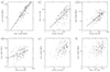 |
Fig. B.1. Scatter plots of some statistical properties for 126 loops. (a) Loop length vs. loop height (Pearson correlation cP= 0.90), (b) Magnetic field strength in the strong vs. weak footpoint of magnetic loop (cP= 0.60), (c) Stronger magnetic field footpoint vs loop height (cP= 0.46), (d) Weaker magnetic field footpoint vs. loop height (cP= 0.45), (e) Stronger magnetic field footpoint vs. loop length (cP= 0.34), and (f) Weaker magnetic field footpoint vs. loop length (cP= 0.31). |
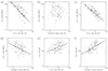 |
Fig. B.2. Scatter plots of some statistical properties for 126 loops. (a) Magnetic field strength at the loop top vs. loop height (Pearson correlation coefficient cP of −0.59), (b) Average magnetic field strength along the loop vs. loop height (cP = −0.30) (c) Magnetic field strength on loop top vs. loop length (cP = −0.64), (d) Average magnetic field strength along the loop vs. loop length (cP = −0.44), (e) Magnetic field strength on loop top vs. loop average intensity (cP = 0.35), (f) Average magnetic field strength along the loop top vs. loop average intensity (cP = 0.58). |
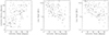 |
Fig. B.3. Scatter plots of magnetic field line inclination relationships. Left: Inclination at the weak B footpoint vs. the strong. Middle: Inclination at the strong B footpoint vs. loop height. Right: Inclination at the weak B footpoint vs. loop height. Linear fits: y = a + bx with a = 23.56 and b = 0.60 for the inclination at the strong vs. the inclination at the weak footpoint. a = 7.01 and b = −0.08 for inclination at strong footpoint vs. loop height. a = 7.07 and b=−0.07 for inclination at weak footpoint vs. loop height. |
All Tables
All Figures
|
Fig. 1. All 126 examples of the uncurled loops.The colour level shows the AIA 193 intensity on a linear scale. The loops are arranged by the loop length. |
| In the text | |
|
Fig. 2. Two examples of loops fitted with the fully (standard) automatic algorithm (cases 1 and 72). Left: AIA 193 intensity with the best field line (black line) fitted a loop. The circles mark the potential footpoint areas as automatically selected by the algorithm. Only closed magnetic field lines with footpoints in these circled areas are considered for the fitting procedure. The three black and green contours indicate negative polarities. The three orange and red contours outline positive polarities. All contours are relative to the absolute maximum field strength in the magnetograms, equispaced between 0 and max |Bz|. The intensity of each image is scaled to the maximum intensity of the image. Right: black curve shows the magnetic field strength along the loop length as obtained from the LMHS model. The red curve gives the loop height along its length. |
| In the text | |
|
Fig. 3. Same as Fig. 2 of cases 4 and 6 for field lines obtained using a non-standard approach. See Section 4.1 for details. |
| In the text | |
|
Fig. 4. Four examples of 3D loop views. The best-computed field lines are shown in black lines that match the observed AIA 193 loops. The observed magnetograms are shown at the bottom of the 3D plots with green/red colours for negative/positive Bz values, respectively. Top row: HMI magnetogram of cases 1 and 72 shown in Fig. 2. Bottom row: same for cases 4 and 6 shown in Fig. 3. |
| In the text | |
|
Fig. B.1. Scatter plots of some statistical properties for 126 loops. (a) Loop length vs. loop height (Pearson correlation cP= 0.90), (b) Magnetic field strength in the strong vs. weak footpoint of magnetic loop (cP= 0.60), (c) Stronger magnetic field footpoint vs loop height (cP= 0.46), (d) Weaker magnetic field footpoint vs. loop height (cP= 0.45), (e) Stronger magnetic field footpoint vs. loop length (cP= 0.34), and (f) Weaker magnetic field footpoint vs. loop length (cP= 0.31). |
| In the text | |
|
Fig. B.2. Scatter plots of some statistical properties for 126 loops. (a) Magnetic field strength at the loop top vs. loop height (Pearson correlation coefficient cP of −0.59), (b) Average magnetic field strength along the loop vs. loop height (cP = −0.30) (c) Magnetic field strength on loop top vs. loop length (cP = −0.64), (d) Average magnetic field strength along the loop vs. loop length (cP = −0.44), (e) Magnetic field strength on loop top vs. loop average intensity (cP = 0.35), (f) Average magnetic field strength along the loop top vs. loop average intensity (cP = 0.58). |
| In the text | |
|
Fig. B.3. Scatter plots of magnetic field line inclination relationships. Left: Inclination at the weak B footpoint vs. the strong. Middle: Inclination at the strong B footpoint vs. loop height. Right: Inclination at the weak B footpoint vs. loop height. Linear fits: y = a + bx with a = 23.56 and b = 0.60 for the inclination at the strong vs. the inclination at the weak footpoint. a = 7.01 and b = −0.08 for inclination at strong footpoint vs. loop height. a = 7.07 and b=−0.07 for inclination at weak footpoint vs. loop height. |
| In the text | |
Current usage metrics show cumulative count of Article Views (full-text article views including HTML views, PDF and ePub downloads, according to the available data) and Abstracts Views on Vision4Press platform.
Data correspond to usage on the plateform after 2015. The current usage metrics is available 48-96 hours after online publication and is updated daily on week days.
Initial download of the metrics may take a while.