| Issue |
A&A
Volume 690, October 2024
|
|
|---|---|---|
| Article Number | A358 | |
| Number of page(s) | 13 | |
| Section | Stellar structure and evolution | |
| DOI | https://doi.org/10.1051/0004-6361/202450042 | |
| Published online | 22 October 2024 | |
Comparison of the disk precession models with the photometric behavior of TT Ari in 2021-2023
1
Institut für Astronomie und Astrophysik, Kepler Center for Astro and Particle Physics, Universität Tübingen, Sand 1, 72076 Tübingen, Germany
2
Parallax Enterprise, Kazan, Russia
3
American Association of Variable Star Observers, 49 Bay State Road, Cambridge, MA 02138, USA
4
AstroMallorca, Palma, Balearic Islands, Spain
5
Space Physics and Astronomy research unit, PO Box 3000 FIN-90014 University of Oulu, Finland
Received:
20
March
2024
Accepted:
19
August
2024
Abstract
We present a comparative analysis of photometric observations of the cataclysmic variable TT Ari in its bright state obtained by the TESS orbital observatory in 2021 and 2023 and by ground-based amateur telescopes in 2022. The light curves from 2021 and 2022 are dominated by modulations with a period slightly shorter than the orbital one (negative superhumps), 0.13292 and 0.13273 d, respectively. From the data obtained in 2023, we see much stronger modulations appearing on a much longer timescale of a few days with an amplitude of up to 0.5 mag, compared to 0.2 mag in 2021. We also find the negative superhump variability with the period of 0.1338 d in the 2023 observations, but the significance of these negative superhumps is much lower than in the previous seasons. We detect less significant additional modulations with a period exceeding the orbital one (positive superhumps) in the observations from 2021 and 2022. Their periods are 0.15106 and 0.1523 d, respectively. We also find a previously unnoticed periodic signal corresponding to the orbital period of 0.13755 d in the TESS observations in 2021. Theoretical models of tidal precession of an elliptical disk predict a decrease in the precession period (and an increase in the period of the positive superhumps) with increasing disk radius, which is consistent with the observed photometric behavior of the system. This enables us to estimate the mass ratio q of the components in TT Ari to be in the range of 0.24–0.29. The tilted disk precession model predicts a period of nodal precession whose value is in general agreement with observations.
Key words: accretion / accretion disks / methods: observational / techniques: photometric / novae / cataclysmic variables / pulsars: individual: TT Ari
Corresponding author; This email address is being protected from spambots. You need JavaScript enabled to view it.
© The Authors 2024
 Open Access article, published by EDP Sciences, under the terms of the Creative Commons Attribution License (https://creativecommons.org/licenses/by/4.0), which permits unrestricted use, distribution, and reproduction in any medium, provided the original work is properly cited.
This article is published in open access under the Subscribe to Open model. This email address is being protected from spambots. You need JavaScript enabled to view it. to support open access publication.
1. Introduction
TT Ari is a bright (about 10.5–11 mag in the V band) cataclysmic variable star belonging to the subclass of the VY Scl stars (anti-dwarf novae), and is available for systematic observations even with small amateur telescopes. This is a binary system consisting of a white dwarf and a late-type (M3.5) main sequence star (Gänsicke et al. 1999). The orbital period Porb of TT Ari, determined from the radial velocity curves, is 0.13755 days (Cowley et al. 1975). Most of the time, the system is in a bright (high) state. Sometimes the brightness of the system decreases from 11 to 17 mag, as in 1983 and 2009 (Koff & Patterson 2010).
Estimates of the mass ratio of the components q and the inclination angle of the orbital plane to the line of sight i are within the limits: 0.19 ≤ q = M2/M1≤ 0.4; 17° ≤ i ≤ 30° according to Cowley et al. (1975), Wu et al. (2002), and Belyakov et al. (2010). Here, M2 is the mass of the secondary donor star, and M1 is the mass of the white dwarf. The system is not eclipsing because of the small inclination angle. However, the brightness of the system varies with an amplitude of a few tenths of a magnitude, with a period close to the orbital but noticeably different from it. This brightness variability was discovered in 1969 (Smak & Stepien 1969) and studied further by other authors (see, e.g., Semeniuk et al. 1987; Andronov et al. 1999; Smak 2013; Bruch 2019). It was shown that the photometric period can be either shorter or longer than the orbital one, and it depends on the mean brightness of the system (Stanishev et al. 2001; Belova et al. 2013). If the brightness of the system is lower than V ≈ 11.3 mag, then the photometric period exceeds the orbital one, while in the brighter state the photometric period is shorter than orbital. Being in a bright state most of the time, the TT Ari system is similar to the nova-like variable V603 Aql, which demonstrates a photometric period longer than the orbital one, but when the system becomes brighter, it transits to a state with a photometric period shorter than the orbital (Patterson et al. 1997; Suleimanov et al. 2004).
The reason for the photometric variability in such systems is still not reliably known. The most plausible explanation is provided by the model of an elliptical precessing accretion disk. In this case, the observed photometric period is the beat period between the orbital period and the disk precession period. Such a model was used to explain the photometric variability of SU UMa-type dwarf novae during especially bright and long outbursts (so-called superhumps during superoutbursts; Osaki 1985), and was confirmed by numerical calculations (Whitehurst 1988). According to these calculations, the disk becomes elliptical due to a 3:1 resonance between the Keplerian period at the outer edge of the disk and the orbital period. This kind of resonance is possible only for a sufficiently small mass ratio of the components, namely of q ≤ 0.3 (or even q < 0.22; see Smak 2020). An elliptical disk precesses in the direction of orbital motion (apsidal precession) and this kind of precession can only explain the photometric periods that exceed the orbital one (positive superhumps).
Patterson et al. (1997) suggested that the accretion disk can be not only elliptical, but also inclined to the orbital plane. In this case, it is also precessing in the direction opposite to the orbital motion (nodal precession). In the restricted three-body problem, the period of the nodal precession is about twice as long as the apsidal precession. If this relationship also exists in the accretion disk precession, this should lead to a well-defined relationship between photometric periods longer and shorter than the orbital one if they are observed in the same system. Indeed, the ratio of the apsidal and nodal disk precession periods is close to 0.5 in the case of V603 Aql (Patterson et al. 1997; Suleimanov et al. 2004).
A search for photometric variability corresponding to the expected precession period of the accretion disk has been attempted by many authors (see, e.g., Semeniuk et al. 1987; Udalski 1988; Kraicheva et al. 1999). The most complete analysis of the system’s photometric behavior, summarizing observations made over the past 40 years, is presented by Bruch (2019). This authors showed, in particular, that the system’s light curves often contain a periodicity that is close to the expected disk precession period but does not coincide with it. Bruch (2022) also performed an analysis of the long (quasi-)continuous photometric observations of the system obtained by the TESS orbital observatory (Ricker et al. 2014). He showed that in addition to the negative superhumps (predominant ones) and positive superhumps, only the beat period between these two photometric periods is reliably detected.
In addition to near-orbital photometric variability, TT Ari exhibits quasi-periodic oscillations with an amplitude of about 0.1 mag and a period of close to 20 minutes (Semeniuk et al. 1987; Udalski 1988; Tremko et al. 1996; Kraicheva et al. 1999; Bruch 2019). The nature of this kind of oscillation has not yet been established. At the same time, other authors do not find significant quasi-periodic oscillations in the range of 15–20 minutes (Vogt et al. 2013) and note that such oscillations are transient, short-lived phenomena (Smak 2014). There is no doubt, however, that there is an excess in the power spectrum of the light curves against a background of red noise in the period range of 10–60 minutes (Kraicheva et al. 1999; Belova et al. 2013).
The aim of the present work is to analyze two long quasi-continuous observations of the cataclysmic variable TT Ari obtained by the TESS observatory in 2021 and 2023, supplemented by our ground-based observations performed in 2022. We search for periodicities associated with the precession of the accretion disk and study the brightness variability of the system on timescales of tens of minutes.
2. Observations
The Transiting Exoplanet Survey Satellite (TESS) orbital observatory is designed primarily for exoplanet searches. However, as a result of its work, relatively long homogeneous time-series of observations of a large number of stars, including cataclysmic variables, become available. In particular, TESS observed TT Ari twice: once in 2021 from August 20 to October 10 in Sectors 42 and 43, and once very recently in 2023 from September 20 to November 11 in Sectors 70 and 71. An analysis of the first TESS observation was presented in Bruch (2022). Here we re-examine this TESS light curve and analyze the second light curve. We then compare the findings with the analysis of our own observations. Throughout the paper, the TESS data sets are referred to as TESS-21 and TESS-23. In the following section, we show that during the TESS-23 observations, around JD 2460240, the photometric behavior of TT Aur changed dramatically. For this reason, we divided the TESS-23 set into two subsets, TESS-23a and TESS-23b. Also, after a short gap in the TESS-21 light curve between JD 2459473 and 2459474, the average brightness of TT Ari decreased by about 0.05 mag, which was accompanied by a change in the character of the variability (see below). These first- and second-half pieces of the TESS-21 light curve are referred to as TESS-21a and TESS-21b. For the convenience of comparison of the TESS data with our own observations, we converted the TESS fluxes F, given in units of electrons per second, into TESS magnitudes T using the relation T = −2.5log10F + ZP, where ZP = 20.44 is the TESS zero-point magnitude based on the values quoted in the TESS Instrument Handbook.
Additional observations of TT Ari were taken with two amateur telescopes from July 2022 to January 2023; a total of 44 nights of data with a total duration of 136 hours were obtained. Observations from 2022 July 17 to 2022 September 16 were carried out using a 5″ Schmidt-Cassegrain telescope installed 15 km northeast of Kazan (Russia) in an area free from urban development and ambient light sources. The CCD camera ZWO ASI-294MC without filters was used as a detector. The duration of each observation was 20-40 seconds. Primary reduction was performed by the standard method using MaxIm DL 5.10 software. The following observations from 2022 September 20 to 2023 January 7 were performed in Palma (Majorca, Balearic Islands, Spain) in a zone of urban development and strong light pollution. A 127-mm Maksutov-Cassegrain telescope with the V filter was used with the CCD camera ZWO ASI533MM. The exposure time of each observation was 60 seconds. Primary reduction was performed using DeepSkyStacker 3.3.2.
Aperture photometry was carried out using the nearby comparison (R) and check (C) stars, whose brightness was taken from the AAVSO database. These stars are indicated in a finding chart of TT Ari in Fig. 1, and their V magnitudes are listed in Table 1.
 |
Fig. 1. Finding chart of TT Ari. |
Comparison stars.
3. Analysis of the variability of TT Ari
Light curves of TT Ari are shown in Fig. 2. In 2021–2023, when the data analyzed here were collected, the system was in a bright state, varying between roughly 10.6 and 11.2 mag. We note that the variability of the system in 2023 differs significantly from its usual photometric behavior. Usually, the variability of TT Ari is dominated by a photometric period close to the orbital one (see, e.g., Bruch 2019). However, the dominant variability timescale was significantly longer in 2023, namely of about a few days.
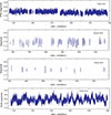 |
Fig. 2. Light curves of TT Ari obtained by TESS in 2021 and 2023 (top and bottom panels, respectively), and in Kazan and Palma de Mallorca in 2022 (two middle panels). |
Using the generalised Lomb-Scargle (GLS) period analysis method (Zechmeister & Kürster 2009) as implemented in PyAstronomy1 (Czesla et al. 2019), we calculated the power spectra of individual data sets. These periodograms exhibit several strong peaks, which can be roughly divided into two groups: those located around the orbital frequency νorb = 7.27 d−1, and those below ∼1 d−1. These two groups of periods are further investigated separately. The period errors given below were also estimated using the PyAstronomy/GLS method, as it delivers an associated error when estimating the period.
To examine the evolution of signals over short time intervals, we also calculated slidograms (i.e., sets of the power spectra calculated with the window moving along the time series) of selected data sets, following the technique of a sliding periodogram (see, e.g., Neustroev et al. 2005). The slidograms were calculated adopting different values of the time-span of the window, which sets the frequency resolution of the power spectrum. For frequencies close to and higher than the orbital one, we settled on the windows of 2–4 days, while for low frequencies we used the window of 10 days as a good compromise between time resolution and frequency resolution. The more homogeneous nature of the TESS data resulted in higher-quality periodograms, which we analyze first before comparing the results with those derived from the two other data sets.
The calculated slidograms were also used to investigate how amplitudes of selected variabilities depend on time during the TESS-21 and TESS-23 observations. To find these amplitudes, the light curves of all the time intervals (windows) were fitted by a sinusoid with the given period.
3.1. Photometric periods close to the orbital period
Bruch (2022) noticed that the remarkable feature of the TESS-21 light curve is the simultaneous presence of negative and positive superhumps (modulations with periods shorter and longer than the orbital one, respectively), something that has never previously been observed in TT Ari. We confirm (see Fig. 3, top left panel) that TESS-21 is indeed dominated by negative superhumps with a period of 0.132920(2) d (ν− = 7.5233(1) d−1 and at least three first harmonics) and a total amplitude of 0.05 mag (see Fig. 3, top right panel, and Table 2). Positive superhumps with the period of 0.15106(1) d are evident in the power spectrum as the peaks at ν+ = 6.6200(6) d−1 (see Fig. 3, bottom left panel) and its first harmonic 2ν+. The amplitude of this periodicity is significantly smaller, about 0.01 mag (Fig. 3, bottom right panel). The beat between these two signals (ν−-ν+) produces a very strong peak at 0.9011(3) d−1 (1.1094(3) d) and peaks at its first two harmonics. This period is the second most important with an oscillation amplitude of approximately 0.03 mag; a more detailed discussion is provided in the following subsection. There is also evidence for a signal at ν−+ν+ = 14.143 d−1. The reliable detection of two photometric periods above and below the orbital one indicates that both the apsidal and the nodal precessions were found simultaneously. This means that the disk was elliptical during the observational interval and at the same time inclined to the orbital plane if the model suggested by Patterson et al. (1997) is correct.
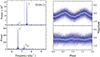 |
Fig. 3. Results from a search for periods around the orbital one in TESS 21 light curves. Left panels: Periodograms of the observed (top panel) and pre-whitened by the ν− frequency (bottom panel) light curves of the TESS-21 observations in the frequency range of 5–10 d−1. The strongest peaks corresponding to the negative (ν−) and positive (ν+) superhumps and the orbital variability (νorb) are labeled. The position of the νorb frequency in the top panel is shown by the vertical dashed line. Right panels: The TESS-21 light curve folded with the negative (top panel) and positive (bottom panel) superhump periods. The phase-binned light curves and their best sinusoid fits are also shown. |
Periods found in the observational intervals: sequentially TESS-21a, TESS-21b, Kazan-22, TESS-23a, and TESS-23b. The periods in different intervals are divided by double lines.
Surprisingly, we also detect a peak at νorb = 7.271(1) d−1 (0.13753(3) d) corresponding to modulations with the orbital period. Although this peak is relatively weak in the original periodogram, it becomes apparent after pre-whitening the light curve with the negative superhumps’ signal (Fig. 3, bottom left panel). The amplitude of the variability with this period is very low, about 0.005 mag. In the past, orbital photometric modulations were detected only during the deep low state and have never been seen in the high state (Bruch 2019, 2022).
It is obvious that the ν+ peak is much less significant than that of ν−. Moreover, the slidogram of TESS-21 (Fig. 4) shows that the positive superhumps were not always visible, and were most significant during the last 10 days of this observation. We also note that the significance of the peak corresponding to the negative superhumps varies during the observation interval of about four days, which is close to the expected period of the inclined accretion disk precession.
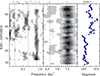 |
Fig. 4. Sliding periodograms (slidograms) in two frequency ranges calculated for the TESS-21 data set, shown as gray-scale images. The slidograms in a low-frequency range of 0.1–1.1 d−1 are calculated with a window of 10 days, while for frequencies close to the orbital one, we used the window of 2 days. The right panel shows the light curve, also smoothed with the window of 2 days. Dashed vertical lines in the slidograms denote the important frequencies discussed in the paper (see text for explanation). |
An analysis of the time dependencies of superhump amplitudes during the TESS-21 observation confirms these conclusions (Fig. 5, top panels). Indeed, when using a sliding window of 1 or 2 days, the amplitude of the negative superhumps shows variability with a typical timescale of 4–5 days. These variations are smoothed at the longer windows. The amplitudes of the positive superhumps increase at the end of the observational set and show variability with the period corresponding to the beat frequency with the period of the negative superhumps ν−-ν+. These beats disappear if the ν− prewhitened light curve is considered. Similar irregular resonances with the negative superhumps are seen in the time dependence of the orbital variability amplitude. They also disappear if the prewhitened light curve is considered.
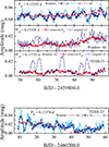 |
Fig. 5. Time dependencies of amplitudes of found photometric modulations with frequencies higher than 1 d−1 for TESS-21 (top panels) and TESS-23 (bottom panel) data sets. |
The periodogram of the Kazan observations obtained roughly 300 days after TESS-21 is generally consistent with that of TESS-21, despite being affected by aliases due to gaps and irregularities present in the data sampling (see Fig. 6, top left panel). This power spectrum is also dominated by the very strong peak at ν− = 7.5340(3) d−1 and its one-day aliases (2ν− is also present). After prewhitening the light curve with this signal, the signal of the positive superhumps at ν+ = 6.5628(9) d−1 becomes apparent (Fig. 6, bottom left panel). The amplitudes of these periodicities are larger than in 2021, measuring 0.065 mag and 0.033 mag, respectively (Fig. 6, right panels). However, the peak corresponding to the beat between these two signals ν−-ν+ = 0.971 d−1 is very weak, in contrast to TESS-21, where it appears to be the second strongest in the periodogram.
Unfortunately, the following observations made in Palma have a large duty cycle and relatively short durations during the nights. Therefore, the corresponding periodogram is heavily affected by an extremely complex window function with large aliasing effects, making it difficult to reliably decipher the exact frequencies of the dominated oscillations. However, the frequency of the strongest peak at 7.5273(3) d−1 is very close to ν− from the Kazan data.
Interestingly, the appearance of the light curve of the TESS-23 data set and its corresponding periodogram are completely different from those of TESS-21. The light curve exhibits strong modulations (with an amplitude of up to 0.5 mag, compared to 0.2 mag in TESS-21) on a relatively long (a few days) timescale. The power spectrum of the entire TESS-23 data set is indeed dominated by low-frequency modulations, which we discuss in Section 3.2, and only shows a weak signal at ν− = 7.476(18) d−1 (0.1338(3)) with a low amplitude of 0.01–0.02 mag (see Fig. 7). The sliding periodogram in the frequency range close to the orbital one demonstrates (Fig. 8) that, on about JD 2460240, TT Ari experienced a transition to a state in which the negative superhumps, which were seen clearly before that date, suddenly almost disappeared. As seen in Fig. 5 (bottom panel), the amplitude of the negative superhumps after this date dropped below 0.01 mag but then began to increase slowly again.
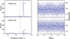 |
Fig. 7. Results from a search for periods around the orbital one in TESS 23 light curves. Left panels: Periodograms of the observed light curves of the TESS-23a (top panel) and TESS-23b (bottom panel) observations in the frequency range of 6–8 d−1. The strongest peak corresponding to the negative (ν−) superhumps is labeled. The position of the νorb frequency is shown by the vertical dashed line. Right panels: TESS-23a (top panel) and TESS-23b (bottom panel) light curves folded with the period of the negative superhumps. The phase-binned light curves and their best sinusoid fits are also shown. |
Due to the presence of this transition, we split the TESS-23 set into two subsets, TESS-23a and TESS-23b, and studied them separately. We find that their periodograms shown in Fig. 7 are not notably different, apart from a much stronger ν− signal in TESS-23a compared to TESS-23b, and somewhat stronger low-frequency signals in TESS-23b than in TESS-23a (see Fig. 9 below). However, even in TESS-23a the ν− signal was much weaker than it was in our previous data sets.
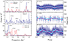 |
Fig. 9. Results of searching long periods in all the investigated light curves. Left panels: Periodograms of the light curves obtained during all the observational intervals in the frequency range of 0.1–1.1 d−1. The vertical dashed lines show the positions of the frequencies corresponding to the expected periods of the nodal (left dashed lines) and apsidal (right dashed lines in the two upper panels) precessions of the tilted elliptical accretion disk. The periods corresponding to the two most stable peaks around periods 2.7–2.9 d and 1.8–1.9 d are marked. A peak corresponding to the observation duty cycle of 1 day is also visible in the middle panel. Right panels: Light curves folded with the most significant low-frequency periods. |
3.2. Low-frequency range: Search for direct evidence of disk precession
All the calculated periodograms show relatively strong peaks at frequencies of ≲1 d−1. In this interval, in addition to modulations at the beat ν−-ν+ frequency, a direct periodic signal from the precession of the accretion disk is expected (see, e.g., Semeniuk et al. 1987; Smak 2013). As mentioned before, photometric periods close to the orbital one, Pph, are interpreted as beat periods between the orbital period Porb and the disk precession period Ppr:
 (1)
(1)
Here, the minus sign is used when the disk precesses in the direction of the orbital motion (apsidal line precession, a positive superhump), and the plus sign is used when the disk precesses in the opposite direction to the orbital motion (tilt disk node line precession, a negative superhump).
Using this expression, we can estimate the expected disk precession periods from the found photometric periods of superhumps. It appears that the period of precession of the line of apsides Ppr+ should have been close to 1.538 and 1.414 d (νpr+ = 0.650 and 0.707 d−1) at the time of the TESS-21 and Kazan observations, respectively, while the period of precession of the line of nodes Ppr− should have been 3.953, 3.788, and 4.831 d (νpr− = 0.253, 0.264, and 0.207 d−1) at the time of the TESS-21, Kazan, and TESS-23a observations, respectively. We note that the derived ratio of precessions Ppr+/Ppr− is almost constant, at 0.39 and 0.37 for the observations in 2021 and 2022, respectively. This ratio is smaller than was expected from the ratio of the precession periods for the Moon (0.47) and that found for V603 Aql (0.47–0.51, Patterson et al. 1997; Suleimanov et al. 2004).
Periodograms in a frequency range of 0.1–1.1 d−1 for all the investigated observational intervals are presented in the left panels of Fig. 9. There are almost no clear peaks at the expected disk precession period, except for the peak at 0.23–0.25 d−1 in TESS-21, which corresponds to νpr− with the low amplitude of about 0.01–0.02 mag. Although this peak is relatively weak, the sliding periodogram demonstrates (Fig. 4, left panel) that the νpr− signal appears much stronger after JD 2459474. Indeed, the peak close to νpr− in the periodogram of TESS-21b is more significant (Fig. 9).
It is interesting that the strengthening of the νpr− modulation in TESS-21b is accompanied by a weakening of the beat signal (ν−-ν+) at 0.901 d−1; see also the top panels of Fig. 10. There was also an appearance of a weak signal with a frequency of close to νpr+ = 0.650 d−1.
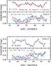 |
Fig. 10. Time dependencies of the amplitudes of the photometric modulations with frequencies of lower than 1 d−1 found in the TESS-21 (top panels) and TESS-23 (bottom panel) data sets. |
In contrast to TESS-21, TESS-23 is dominated by low-frequency modulations, which produce several strong peaks in the periodogram (Fig. 9, left panels). However, the corresponding slidogram (Fig. 8, left panel) indicates that all these signals have a low degree of coherence. Nevertheless, during the first half of TESS-23, and also later in this time interval, there was a very strong signal with a frequency of close to νpr−, namely 0.234 d−1. The amplitude of this periodicity is about 0.1 mag (see the right panels of Fig. 9 and the bottom panels of Fig. 10).
There are also a few other prominent peaks in the presented periodograms, whose frequencies are close to each other in different time intervals. These peaks correspond to periods of 2.75 d and 1.81 d (TESS-21), 2.95 d and 1.82 d (Kazan-22), and 2.73 d and 1.88 d (TESS-23b); see Fig. 9. We note that the amplitudes of these periodicities increase in the second halves of both the TESS observations and that, during the TESS-23 observation, the amplitudes of low-frequency oscillations are a few times larger than during other observations (see Fig. 10). A period of close to 2.95 d was also detected earlier by other observers (e.g., 2.92 d, Andronov et al. 1999). Formally, a peak that corresponds to the beat frequency ν−-ν+ ≈ 0.968 d−1 (1.033 d) exists in the periodogram of the Kazan observations (see Fig. 9), but the significance of this peak is low. All of the periods found in the investigated frequency range are collected in Table 2.
3.3. Quasi-periodic oscillations on a scale of tens of minutes
A study of the quasi-periodicity of the system was carried out in the range of periods from 5 to 60 minutes using all the observed intervals. For the ground-based data (Kazan and Palma), this analysis was conducted for each night with a duration of observation of longer than 1.5 hours. The most frequently observed periods are in the range of 15–30 minutes with a brightness amplitude of about 0.02 mag. At the same time, we note that periods of about 15 and 27 minutes can be repeated over two or three consecutive nights. As an example, Fig. 11 (left-hand panel) shows the periodogram and how the periodogram changes during the night for the light curve obtained on 2023 January 7. It can be seen that the found period is not constant, but varies over times comparable with the period itself. At the end of the night, the frequency of this peak drifts towards lower frequencies. This is the most significant period found in the interval under study and is close to the periods noted earlier as periods of quasi-periodic oscillations in the system (Semeniuk et al. 1987).
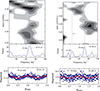 |
Fig. 11. Examples of searching for quasi-periodic oscillation in ground-based light curves. Top panels: Slidograms in the range of periods of 15–60 minutes during the nights 2023 January 7 (left panel) and 2022 August 1 (right panel). Middle panels: Corresponding periodograms in the same range of periods for the same nights. Bottom panels: Light curves folded with the most significant periods. |
Another example is shown in the right panel of Fig. 11, this time for the night of 2022 August 1. The periodogram of this night also shows a fairly significant period of 20 minutes. However, the corresponding slidogram demonstrates that no stable modulations with any characteristic period were present throughout the night. Moreover, the peaks in the night-averaged periodogram do not correspond exactly to the emerging short-period modulations seen in the slidogram.
Results of the TESS observations are presented in the sliding periodograms in the range of periods of 15–60 minutes (Fig. 12). All the peaks appearing in this interval of periods are short-lived.
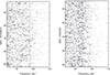 |
Fig. 12. Slidograms in the frequency range of 20–150 d−1 during the entire TESS-21 (left panel) and TESS-23 (right panel) observations. The vertical dashed lines show the positions of the break frequencies νc, 90 d−1 (TESS-21) and 72 d−1 (TESS-23). |
We also computed wide-range power spectra of the observed light curves corresponding to all the observed intervals, excluding Palma observations. The results are presented as separate power spectra in log-log scale (Fig. 13). Every power spectrum can be described by a power law (red noise) and some additional noise component making the power spectrum flat at the frequencies between approximately 10 d−1 and 100 d−1. The excess noise can be described by the analytical function:
 (2)
(2)
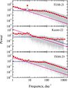 |
Fig. 13. Total power spectra (gray curves) in log-log scale obtained using TESS-21 (top panel), Kazan-22 (middle panel), and TESS-23 (bottom panel) observations. The red circles show the averaged power spectra. The magenta lines show the power law with an exponent of −2, and the blue curves are the fits of the excess power spectra, represented by the formula (2) with the parameters A = 5, νc = 90 d−1, and γ = 2.2 (TESS-21), A = 2.7, νc = 90 d−1, and γ = 2.2 (Kazan-22), and A = 7, νc = 72 d−1, and γ = 2.2 (TESS-23). |
The red noise, which probably arises due to random viscosity fluctuations in the accretion disk (Lyubarskii 1997), can be approximated by the power law with an exponent of −2 in all the observational intervals. The exponent γ = 2.2 describing the additional noise spectra, is also the same for all the power spectra, but the power level in the TESS observations is higher, that is, A = 5 (TESS-21) and A = 7 (TESS-23) versus A = 2.7 (Kazan-22). The break frequencies are identical for power spectra obtained using observations in 2021 and 2022, at νc = 90 d−1, but appears lower in the TESS-23 observations, νc = 72 d−1. The higher accuracy of the TESS observatory data makes it possible to trace the red noise of the additional component up to the Nyquist frequency (≈4000 d−1), and towards low frequencies down to the characteristic frequencies corresponding to several days. The power spectrum of the Kazan observations is similar in appearance to the TESS power spectra. Due to limitations imposed by ground-based observations, the high frequencies above ∼200 d−1 are not available for analysis.
These results confirm previous conclusions (Kraicheva et al. 1999; Smak 2013; Bruch 2019), namely that the system TT Ari shows no quasi-periodic brightness oscillations, and its variability at times of 10–60 minutes is stochastic noise, among which quite significant variability sometimes appears at some characteristic frequency from a given interval.
4. Comparison with precession models and estimations of the system parameters
4.1. Elliptical disk precession
According to the current concepts, the disk becomes elliptical and begins to precess towards orbital motion when it expands beyond the 3:1 resonance radius R3 : 1 (Whitehurst 1988; Osaki 1989):
 (3)
(3)
where rres is a relative disk radius, and a is the semi-major axis of the orbit (formula (5.125) in Frank et al. 2002).
The period of precession  and the corresponding period of positive superhumps
  – to the formation of which the precession contributes –, depend on the mass ratio q. The superhump period excess
  can potentially be calibrated using accurate values of q and observed values of ε+. Several such empirical relationships between ε+ and q have been obtained based on observations of cataclysmic variables (mostly of SU UMa-type stars) showing positive superhumps (see, e.g., Patterson et al. 2005; McAllister et al. 2019, and references therein). Using the dependence proposed by Patterson et al. (2005),
 (4)
(4)
and adopting the values of ε+ observed in TT Ari ( varies between 0.1483 and 0.1523 days (Bruch 2019, and this work), and therefore ε+ is within 0.078-0.107), one obtains a mass ratio of within 0.29 – 0.37.
It must be noted that all the existing relationships are poorly calibrated at the larger ε+ values end, which is populated by only a few systems with longer Porb and higher q. These stars are not of SU UMa type but are nova-like systems that display permanent superhumps, for which accurate measurements of system parameters, and in particular q, are not available. For example, four such systems from Tables 3 and A1 of McAllister et al. (2019) cover ε+ in the range of 0.063–0.069 and were measured to have a q of between 0.24 and 0.31 with an accuracy of ∼20%. Thus, to estimate q in TT Ari, we have to rely on extrapolation. Despite this, the estimate of q ≈ 0.30 corresponding to ε+ = 0.078 appears reasonable (see figure 7 in McAllister et al. 2019).
This value of q is close to the critical mass ratio qcr at which a binary system may still possess positive superhumps. The exact value of qcr is not known but is commonly accepted to be within 0.30–0.35 based on various theoretical and numerical studies (e.g. Pearson 2006; Wood et al. 2011; Thomas & Wood 2015). There is a natural condition for the existence of qcr, namely the outer disk radius must be at least as large as the 3:1 resonance radius. The outer disk boundary is defined by the tidal interaction with the secondary star. At some distance from the primary, the tidal and viscous stresses become comparable and truncate the disk (Paczynski 1977; Papaloizou & Pringle 1977; Ichikawa & Osaki 1994). The outer disk boundary can be calculated as the largest streamline (the truncated orbit) in the restricted three-body problem that does not cross any other periodic orbit (Paczynski 1977). We note that periodic orbits at large distances from the primary deviate from a circular Keplerian flow and cannot be characterised by a single parameter2 as these streamlines are elongated perpendicular to the lines of centre of the two stars.
Adopting the approach by Paczynski (1977), Smak (2020) recently presented an approximation formula for the orbit-averaged radius of the truncated orbit:
 (5)
(5)
Although the meaning of rRoche is not given in the paper, we can confirm, based on our calculations, that it is the volume radius of the Roche lobe of the white dwarf. It can be approximated using, for example, a formula by Eggleton (1983):
 (6)
(6)
Based on the fact that the intersection of the two relations (3) and (5) gives q = 0.22, Smak (2020) questioned the origin of positive superhumps due to the 3:1 resonance in higher q systems. However, most of the recent SPH simulations, which treat tidal effects accurately, still show the appearance of the superhumps in binaries with a much higher mass ratio of up to q≈0.35 (e.g., Wood et al. 2009). There may be several reasons for this disagreement.
First, Smak (2020), in his analysis, considered a simple case of circular orbits. However, it is well known that the width of the 3:1 resonance depends strongly on the eccentricity (e.g., Hadjidemetriou 1993), and all the orbits in the outer disk are highly noncircular. For example, using Eq. (5) for a system with q = 0.300, one obtains the orbit-averaged circular radius rtid/rRoche = 0.872. In reality, this orbit is highly elongated, which should significantly widen the resonance range. Indeed, using an approximation formula for rmax from Neustroev & Zharikov (2020),
 (7)
(7)
one can obtain rmax/rRoche = 0.951, while r1/rRoche = 0.782 and r2/rRoche = 0.790.
Second, to calculate the truncated disk radius, Paczynski (1977) adopted the inviscid three-body formalism. However, accretion disks are not collections of noninteracting test particles, but are hydrodynamical flows where gas pressure effects could be potentially important. Indeed, Goodman (1993) demonstrated (see his Fig. 3) that if radial pressure gradients are not neglected, then the disk in systems with q ≳ 0.15 can expand beyond the Paczynski’s radius. From the observational point of view, there exists observational evidence that accretion disks in some cataclysmic variables are extended all the way to rL and that the matter can even escape from the disk in the orbital plane (see, e.g., Kato et al. 2008; Hernandez et al. 2017; Neustroev & Zharikov 2020; Subebekova et al. 2020; Zamanov et al. 2024).
Thus, taking the above into account, in the following we assume that the positive superhumps observed in TT Ari originate from a large precessing elliptical disk, which can be explained by the resonance model. As the changes in the period of the positive superhumps are much greater than the errors in its determination, the obtained interval of the mass ratio 0.29–0.37 cannot be considered to be the result of statistical errors. The actual value of q, of course, does not change. Consequently, we suggest that the changes in the period of the superhumps are associated with a change in the outer radius of the disk. This means that the lowest value of ε+ corresponds to the case of the outer disk radius equal to the 3:1 resonance radius3, and the increase in ε+ is connected with the increase in the outer disk radius. Here we point out again that the values 0.29 and 0.37 may be quite inaccurate, as they were estimated in the extrapolation regime.
Following Pearson (2006) (see also Lubow 1992; Montgomery 2001), we consider the dependence of the excess of the positive superhumps’ period on the tidal and pressure forces as
 (8)
(8)
where νpr+ is the frequency of the apsidal precession of the eccentric accretion disk. Hirose & Osaki (1990) derived an expression connecting the ratio of the precession frequency of an elliptical disk to the orbital frequency with the relative disk radius r and the mass ratio q. This can be represented as a series:
 (9)
(9)
For our purposes, it suffices to confine ourselves to the first five terms of the series. The contribution of the higher-order terms is negligible. The values of the corresponding coefficients cn are taken from Pearson (2003) and presented in Table 3.
Coefficients cn.
According to Lubow (1992), the precession frequency caused by the pressure effects can be presented as the following equation:
 (10)
(10)
where as is the sound speed at the considered disk radius R, k is a radial wave number, and 2πνp is an angular rotation frequency of the disk matter at this radius. The radial wave number can be determined by using the pitch angle β of a spiral density wave generated by both tidal and pressure forces:
 (11)
(11)
Assuming Kepler orbital motion in the disk, we can relate the frequency of the orbital motion to the orbital frequency:
 (12)
(12)
Finally, the expression for the ratio νpress/νorb can be obtained in the commonly accepted form:
 (13)
(13)
First of all, we estimate the mass ratio in the system assuming that the smallest value of ε+ = 0.078 corresponds to the situation where the outer accretion disk radius is equal to the resonance radius. From the simultaneous solution of equations (3) and (8), we obtain that q ≈ 0.235, if we ignore pressure effects. The pressure effects decelerate the precession frequency, and therefore we expect the mass ratio to be larger if we take into account pressure effects.
The value of νpress/νorb depends not only on the disk radius and the mass ratio but also on the large semi-axis of the system orbit a, the sound speed on the given radius as, and the pitch angle of the spiral waves β. Montgomery (2001) showed from her numerical simulations that the pitch angle is between 13 and 21 degrees. We use these limits on β in our further estimations. We also assume that the accretion disk in TT Ari is in a quasi-permanent hot state during the observations, and therefore that hydrogen is (almost) fully ionized and that the plasma temperature on the outer disk radius is about 104 K. Therefore, we considered two values of the sound speed, 10 and 7.5 km s−1. The first value approximately corresponds to the isothermal sound speed for plasma temperature 104 K, and we also consider the possibility that the plasma temperature could be lower. For the computation of the a value, we assume that the white dwarf mass is 0.8 solar masses.
Incorporating the assumptions described above, we find that the q value is between 0.24 (as = 7.5 km s−1 and β = 21°) and 0.29 (as = 10 km s−1 and β = 13°) if taking into account the pressure effects. In all the cases considered, the resonance radius rres (see Eq. (3)) is larger than the tidal radius rtd (see Eq. (5)) by 1–3%. We also calculated the outer disk radius necessary to reach the maximum observed value of ε+ = 0.107. In all the cases considered, this radius is about 99% of rL, determined by Eq. (6).
Thus, we conclude that, at q = 0.24 − 0.29, the tidal resonance model is the cause of the precession of an elliptical disk, which is in agreement with the observations if we admit that the outer disk radius can be larger than the critical radius rtd determined by Paczynski (1977). In accordance with the model, the increase in the period of the positive superhumps is caused by an increase in the outer radius of the disk. We also conclude that the upper possible value of q ≈ 0.29 is in accordance with the estimation using Patterson’s empirical relation (4).
Based on the above calculations, we can estimate the masses of the components in the system. Several empirical and theoretical relationships exist in the literature between the orbital period and the donor mass in cataclysmic variables, most of which predict a similar value of M2 for the orbital period of TT Ari, of namely Porb = 3.3 hours. For example, the empirical relation by Patterson et al. (2005),
 (14)
(14)
where Porb is expressed in hours, gives M2 ≈ 0.22 M⊙. A more recent, semi-empirical broken-power-law donor sequence for cataclysmic variables from Knigge et al. (2011) predicts M2 to be ≈0.21 M⊙. For further estimations, we assume that the mass of the donor star is 0.18–0.24 M⊙, which gives a mass of the white dwarf of 0.62–1 M⊙ at q = 0.24 − 0.29.
4.2. Tilted disk precession
We show above that the increase in the period of the positive superhumps can be connected to the increase in the outer radius of the accretion disk. The positive superhumps dominate when their period is relatively short, 0.148–0.149 days (see Table 3 in Bruch 2019). However, when the period of the positive superhumps reaches 0.150–0.151 days, the domination of the negative superhumps begins. In particular, in the observations presented above, which were performed in 2021 and 2022, the negative superhumps dominate, although the relatively weak positive superhumps were also present, and their period was above 0.151 d. Therefore, in the framework of the interpretation of the negative superhumps as a precession of the tilted disk and the above suggestion that the increase in the period of the positive superhumps is connected to the expansion of the outer disk radius, this leads to the suggestion that the disk becomes inclined (at least near the outer radius) after reaching some boundary radius.
We also note that the transition4 from the positive to negative superhumps in TT Ari has been associated with a brightness increase, which can also be related to an increase in the outer disk radius (see e.g., Suleimanov et al. 2004). The disk precession model of TT Ari presented above shows that the period of the positive superhumps of about 0.150–0.151 d corresponds to the relative disk radius of about r ≈ 0.47 − 0.48. We hereafter refer to this relative outer disk radius as the transition radius.
The brightness variability of the system when a tilted disk exists is most probably connected with changes in the apparent area of the disk. The apparent area of the tilted disk varies because of changes in the inclination angle to the line of sight due to orbital motion and precession. In Fig. 14, two positions of the accretion disk are shown. The positions correspond to two almost opposite orbital phases. In the first position, a brightness is maximal because the angle between the line of sight and the normal to the disk plane is minimal, i − θ. In the second position, which shifts approximately on the orbital phase angle π, the brightness is minimal at the maximum value of the angle defined above, i + θ. Here, θ is the angle of inclination of the disk to the orbital plane of the system. The difference between the orbital phases of these two accretion-disk positions is slightly less than π due to the nodal precession of the disk.
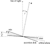 |
Fig. 14. Geometry of the tilted disk precession. Here, n is a normal to the orbital plane, and the normal to the tilted accretion disk plane rotates around n with the period of the negative superhumps. |
The light curves of the system show sine-like variations with a period close to the orbital one (see e.g., Fig. 8). This means that the angle θ is always less than i; otherwise the light curve would be of a double-wave form. As the angle i is small, the inclination of the disk to the orbital plane must also be small. We note that the accretion disk can be inclined at the outer radii only, with the disk plane coinciding with the orbital plane at the central parts.
If we assume that the disk inclines to the orbital plane when the outer radius of the disk reaches the transition radius, it is logical to suggest that with a further increase in the disk radius, the inclination angle will also increase. The amplitude of brightness variability should also increase accordingly. Indeed, the measurements given in Table 3 of Bruch (2019) demonstrate that the amplitude of brightness variations of TT Ari increases with the value of ε− (see Fig. 15). Moreover, from the observations showing both types of superhumps simultaneously, we see that with an increase in ε+ between the TESS-21 and Kazan observations, the value of the corresponding negative superhump period deficit  also increased (see Table 2). Thus, these observational facts support the idea that both an increase in the tilted angle of the disk and an increase in ε− are associated with an increase in the outer radius of the disk.
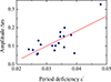 |
Fig. 15. Dependence of the amplitude of the system’s brightness change on the negative superhump period deficit ε− according to Table 3 in Bruch (2019). |
The dynamics of a tilted disk have been studied many times. Such studies are commonly based on the precession of a point mass on an inclined orbit (with respect to the orbital plane) around a white dwarf under the gravitational influence of the secondary component (see, e.g., Montgomery 2009, and references therein). Based on Montgomery’s paper, in which she considers the accretion disk as a collection of such particles uniformly precessing together, like a solid body, we obtain a formula relating the ratio of the precession frequency to the orbital frequency νpr−/νorb with disk radius and disk inclination to the orbital plane θ:
 (15)
(15)
As mentioned above, the transition to a tilted disk possibly occurs at r ≈ 0.47 − 0.48, and the relative disk radius cannot be larger than rL ≈ 0.49 − 0.504 (for the largest and the smallest possible q, 0.29 and 0.24, correspondingly). Therefore, according to (15), the value of the frequency ratio turns is found to be within (0.034 − 0.04) cos θ. The period of negative superhumps varies from 0.1323 days (Belova et al. 2013; Kim et al. 2009) to 0.13424 days (Kraicheva et al. 1999), which results in frequency ratio values of from 0.04 to 0.025. Therefore, the observed values are close to the computed values, because the angle θ is small and cos θ ≈ 1.
The formal application of expression (15) to observational data requires the value cos θ > 1 at the smallest observed values Pph− and q < 0.29. This may be due to the fact that the numerical coefficient in equation (15) is not known precisely, because it depends on the disk surface density distribution along the radius (see, e.g., Larwood 1998). The value 15/32 was obtained in the homogeneous disk approximation, which is generally not true. However, we also suggest that the mass ratio is, in reality, closer to the found upper limit of q ≈ 0.29, or could be even larger if the pressure effects are more significant than assumed.
We note that the above consideration is applicable to the usual state of TT Ari, where the negative superhumps dominate, as they do in 2021 and 2022. The light curve observed in 2023 cannot be explained by the simple toy model presented above. One can speculate that the accretion disk was so highly tilted that the gas stream met the disk at a much smaller radius than the outer disk radius, creating a bright spot inside the disk. This bright spot, which is visible during only half of the inclined disk precession period, can potentially generate the variability of the system brightness on a timescale of a few days.
4.3. Low-frequency periodicities
Here we speculate about possible reasons for the observed low-frequency periodicities. The most interesting is the periodicity near the beat frequency ν− − ν+ observed in 2021 by the TESS observatory. This beat frequency can also be presented as a sum of the expected precession frequencies νpr− + νpr+.
It is important to note that the ratio νorb/(ν− − ν+) ≈ 1.107 d/0.13755 d ≈ 8. Therefore, this beat frequency is close to being in resonance with the orbital motion. We note that the sum of the nodal and the apsidal precession frequencies of the orbit of the Moon is also in resonance with the orbital period of the Earth, 1/18.6 yr + 1/8.8 yr ≈ 1/6. This similarity could be considered to be an additional argument in favor of the idea that the observed negative and positive superhumps are connected with the precession of the elliptical tilted accretion disk, in accordance with the model suggested by Patterson et al. (1997). On the other hand, the ratio of the beat frequency with a low significance, observed in 2022, is close to being in the resonance 2:15, 1.033 d/0.13755 d ≈ 7.5.
In all the observations presented here, there are two approximately stable periodicities at the periods 1.83–1.88 d and 2.73–2.95 d. It is possible to connect the first group of periods with the apsidal precession period at the resonance radius rres. Indeed, if we convert the period 1.88 d to the positive superhump period, we obtain a value that is close to the minimal observed positive superhump period in the system TT Ari, of namely 0.1484 d (see Table 3 in Bruch 2019), and a period excess of ε+ ≈ 0.078. This value coincides with the value that we used in Sect. 4.1 to find the resonance radius. Therefore, we can suggest that the 3:1 resonance instability arises at the resonance radius, and we directly observe this precession period. The instability wave transfers to the outer disk radius with the decreasing precession period, and the observed period of the negative superhumps forms as a beat period between the precession period near the outer disk radius and the orbital period. The reason for the flux variation could simply be the change in brightness of the place of the accretion stream and the accretion disk interaction.
The second group of the periods, 2.73–2.95 d, can be connected with the nodal precession of the tilted accretion disk. These periods can be converted to the periods of the negative superhumps using relation (1), namely 0.1310–0.1314 d. The corresponding period deficits, ε−, are 0.044–0.048. Such low negative superhump periods were never observed and the values of ε− expected from Eq. (15) are smaller for the obtained q range. Nevertheless, we speculate that the considered group of periods correspond to the nodal precession of the tilted accretion disk with the radius close to the Roche lobe radius, whereas Eq. (15) downplays the deficit of the period. This may mean that the accretion disk always extends almost up to the Roche lobe radius, but the negative superhumps correspond to the smaller radius, which can be connected with the place of the accretion stream and the accretion disk interaction.
5. Summary and concluding remarks
This paper presents a comparative analysis of photometric light curves of the cataclysmic variable TT Ari obtained by the TESS orbital observatory in 2021 and 2023, and derived from long ground-based observations in 2022 carried out with amateur telescopes. The observational data and the performed analysis complement the recent extended studies of this cataclysmic variable star (Bruch 2019, 2022).
The system was in a bright state during all of the observational runs presented here. The variability was relatively consistent in its characteristics throughout 2021–2022, predominantly showing a slightly shorter photometric period than the orbital one; this variability is interpreted as negative superhumps from a tilted accretion disk. However, the 2023 light curve exhibits much stronger modulations on a much longer timescale of a few days, with an amplitude of up to 0.5 mag, compared to 0.2 mag in 2021. Previously, dominant negative superhump modulations with a total amplitude of ∼0.10–0.12 mag were found at the beginning of the 2023 data set to have a much milder amplitude of ∼0.04 mag. Moreover, we observe for the first time that, in the second half of the 2023 observational period, TT Ari experienced a transition to a state in which the amplitude of the negative superhumps became even smaller.
In 2021–2022, in addition to the negative superhumps, TT Ari also showed positive superhumps and modulations with the orbital period. The simultaneous presence of all three types of modulation has never previously been observed in TT Ari. The detection of both positive and negative superhumps in the light curves strongly suggests that both the apsidal and the nodal precessions of the accretion disk in TT Ari were found simultaneously. Thus, in 2021–2022, the disk was elliptical and also inclined to the orbital plane, that is, if the interpretation suggested by Patterson et al. (1997) is correct.
We looked for low-frequency photometric modulations directly related to the nodal and/or apsidal precessions of the disk. No strong evidence for such modulations was found, although a periodicity close to that expected for the nodal disk precession is seen in the first half of the 2023 observations. On the other hand, calculated periodograms show a few prominent low-frequency peaks whose frequencies are close in different time intervals. The nature of these modulations is unclear.
The broad-band power spectra of the TESS and ground-based data are consistent with each other. In general, they can be described by red noise, a power law with an exponent of −2, and with an additional signal superimposed on it, which makes a spectrum flat up to the frequency νc = 90 d−1 (72 d−1 in 2023) and then falls off as a power law at higher frequencies with an exponent of −2.2. The difference in the level of this additional noise component and red noise is maximal near νc, corresponding to a period of 16–20 minutes. On some nights, this resulted in peaks in the periodograms at frequencies corresponding to 15–30 minutes. However, the periodicity corresponding to these peaks appears to be short-lived. This confirms the conclusions of other authors (see, e.g., Smak 2014) that the quasi-periodic oscillations on time intervals of 10–60 minutes in TT Ari are short-lived and that the corresponding variability resembles stochastic noise.
We combined the results we obtained with those summarized by Bruch (2019) and compared them with predictions based on theoretical models of accretion disk precession in binary systems. Here we assume that the resonance model suggested by Osaki (1985) is acceptable for the description of the photometric properties of TT Ari, although it requires the resonant radius to be larger than the tidal radius. Thus, we assume that the accretion disk in one or another form exists at radii greater than the boundary radius, as determined by Paczynski (1977). Application of the model of the elliptical accretion disk precession allowed us to find the mass ratio of the components in the system, q, which we find to be in the range of 0.24–0.29. The uncertainty arises from the ambiguity of the pressure effects taken into account. The larger the pressure effect, the larger q.
We interpret the increase in the period of the positive superhumps as an expansion of the outer disk radius. It is important that the outer disk radius is less than the equivalent Roche lobe radius, even for the largest observed period of positive superhumps. This means that our assumption does not lead to any contradictions. However, if we were to find a superhump period that is significantly longer than the maximum period observed yet, this would mean that our assumption is wrong.
Our model of tilted disk precession predicts values for the precession period that are broadly consistent with observations. The previously proposed suggestion that the amplitude and the period of negative superhumps increase with increasing disk radius is also in agreement with observations.
The use of various empirical relations between the mass of the secondary M2 and the orbital period allowed us to estimate the secondary mass M2 to be in the range of 0.18 − 0.24 M⊙, whereas we find the white dwarf mass M1 to be 0.62 − 1 M⊙.
To describe the largest streamlines, Paczynski (1977) used two radial extrema r1 and r2, and the largest radius rmax.
More accurately, the disk has the radius at which the 3:1 resonance starts affecting the disk.
Sometimes the negative and positive superhumps are observed simultaneously, although usually one of them dominates over the other. Therefore, there has to be some time interval when the dominance of one type of superhump modulations is replaced by the other type. It seems natural to call this time interval a transition period, and the corresponding event a transition.
Acknowledgments
The authors thank the Referee for the very useful remarks and suggestions, and Alexander Tokranov for his help with the English language. VFS thank the Deutsche Forschungsgemeinschaft (DFG) for financial support (grant WE 1312/59-1). VN acknowledges the financial support from the visitor and mobility program of the Finnish Centre for Astronomy with ESO (FINCA), funded by the Academy of Finland grant nr 306531.
References
- Andronov, I. L., Arai, K., Chinarova, L. L., et al. 1999, AJ, 117, 574 [NASA ADS] [CrossRef] [Google Scholar]
- Belova, A. I., Suleimanov, V. F., Bikmaev, I. F., et al. 2013, Astron. Lett., 39, 111 [NASA ADS] [CrossRef] [Google Scholar]
- Belyakov, K. V., Suleimanov, V. F., Nikolaeva, E. A., & Borisov, N. V. 2010, AIP Conf. Ser., 1273, 342 [NASA ADS] [Google Scholar]
- Bruch, A. 2019, MNRAS, 489, 2961 [NASA ADS] [CrossRef] [Google Scholar]
- Bruch, A. 2022, MNRAS, 514, 4718 [NASA ADS] [CrossRef] [Google Scholar]
- Cowley, A. P., Crampton, D., Hutchings, J. B., & Marlborough, J. M. 1975, ApJ, 195, 413 [NASA ADS] [CrossRef] [Google Scholar]
- Czesla, S., Schröter, S., Schneider, C. P., et al. 2019, PyA: Python astronomy-related packages, Astrophysics Source Code Library [record ascl:1906.010] [Google Scholar]
- Eggleton, P. P. 1983, ApJ, 268, 368 [Google Scholar]
- Frank, J., King, A., & Raine, D. J. 2002, Accretion Power in Astrophysics: Third Edition (Cambridge, UK: Cambridge University Press) [Google Scholar]
- Gänsicke, B. T., Sion, E. M., Beuermann, K., et al. 1999, A&A, 347, 178 [Google Scholar]
- Goodman, J. 1993, ApJ, 406, 596 [NASA ADS] [CrossRef] [Google Scholar]
- Hadjidemetriou, J. D. 1993, Celest. Mech. Dyn. Astron., 56, 563 [NASA ADS] [CrossRef] [Google Scholar]
- Hernandez, M. S., Zharikov, S., Neustroev, V., & Tovmassian, G. 2017, MNRAS, 470, 1960 [NASA ADS] [CrossRef] [Google Scholar]
- Hirose, M., & Osaki, Y. 1990, PASJ, 42, 135 [NASA ADS] [Google Scholar]
- Ichikawa, S., & Osaki, Y. 1994, PASJ, 46, 621 [NASA ADS] [Google Scholar]
- Kato, T., Maehara, H., & Monard, B. 2008, PASJ, 60, L23 [NASA ADS] [CrossRef] [Google Scholar]
- Kim, Y., Andronov, I. L., Cha, S. M., Chinarova, L. L., & Yoon, J. N. 2009, A&A, 496, 765 [NASA ADS] [CrossRef] [EDP Sciences] [Google Scholar]
- Knigge, C., Baraffe, I., & Patterson, J. 2011, ApJS, 194, 28 [Google Scholar]
- Koff, R. A., & Patterson, J. 2010, Soc. Astron. Sci. Ann. Symp., 29, 83 [Google Scholar]
- Kraicheva, Z., Stanishev, V., Genkov, V., & Iliev, L. 1999, A&A, 351, 607 [NASA ADS] [Google Scholar]
- Larwood, J. 1998, MNRAS, 299, L32 [NASA ADS] [CrossRef] [Google Scholar]
- Lubow, S. H. 1992, ApJ, 401, 317 [NASA ADS] [CrossRef] [Google Scholar]
- Lyubarskii, Y. E. 1997, MNRAS, 292, 679 [Google Scholar]
- McAllister, M., Littlefair, S. P., Parsons, S. G., et al. 2019, MNRAS, 486, 5535 [NASA ADS] [CrossRef] [Google Scholar]
- Montgomery, M. M. 2001, MNRAS, 325, 761 [NASA ADS] [CrossRef] [Google Scholar]
- Montgomery, M. M. 2009, ApJ, 705, 603 [NASA ADS] [CrossRef] [Google Scholar]
- Neustroev, V. V., & Zharikov, S. V. 2020, A&A, 642, A100 [NASA ADS] [CrossRef] [EDP Sciences] [Google Scholar]
- Neustroev, V. V., Zharikov, S., Tovmassian, G., & Shearer, A. 2005, MNRAS, 362, 1472 [NASA ADS] [CrossRef] [Google Scholar]
- Osaki, Y. 1985, A&A, 144, 369 [NASA ADS] [Google Scholar]
- Osaki, Y. 1989, PASJ, 41, 1005 [NASA ADS] [Google Scholar]
- Paczynski, B. 1977, ApJ, 216, 822 [CrossRef] [Google Scholar]
- Papaloizou, J., & Pringle, J. E. 1977, MNRAS, 181, 441 [NASA ADS] [CrossRef] [Google Scholar]
- Patterson, J., Kemp, J., Saad, J., et al. 1997, PASP, 109, 468 [CrossRef] [Google Scholar]
- Patterson, J., Kemp, J., Harvey, D. A., et al. 2005, PASP, 117, 1204 [Google Scholar]
- Pearson, K. J. 2003, MNRAS, 346, L21 [CrossRef] [Google Scholar]
- Pearson, K. J. 2006, MNRAS, 371, 235 [NASA ADS] [CrossRef] [Google Scholar]
- Ricker, G. R., Winn, J. N., Vanderspek, R., et al. 2014, SPIE Conf. Ser., 9143, 914320 [Google Scholar]
- Semeniuk, I., Schwarzenberg-Czerny, A., Duerbeck, H., et al. 1987, Acta Astron., 37, 197 [NASA ADS] [Google Scholar]
- Smak, J. 2013, Acta Astron., 63, 453 [NASA ADS] [Google Scholar]
- Smak, J. 2014, Acta Astron., 64, 167 [NASA ADS] [Google Scholar]
- Smak, J. 2020, Acta Astron., 70, 313 [NASA ADS] [Google Scholar]
- Smak, J., & Stepien, K. 1969, Commmun. Konkoly Obs. Hungary, 65, 355 [NASA ADS] [Google Scholar]
- Stanishev, V., Kraicheva, Z., & Genkov, V. 2001, A&A, 379, 185 [NASA ADS] [CrossRef] [EDP Sciences] [Google Scholar]
- Subebekova, G., Zharikov, S., Tovmassian, G., et al. 2020, MNRAS, 497, 1475 [Google Scholar]
- Suleimanov, V., Bikmaev, I., Belyakov, K., et al. 2004, Astron. Lett., 30, 615 [NASA ADS] [CrossRef] [Google Scholar]
- Thomas, D. M., & Wood, M. A. 2015, ApJ, 803, 55 [NASA ADS] [CrossRef] [Google Scholar]
- Tremko, J., Andronov, I. L., Chinarova, L. L., et al. 1996, A&A, 312, 121 [NASA ADS] [Google Scholar]
- Udalski, A. 1988, Acta Astron., 38, 315 [NASA ADS] [Google Scholar]
- Vogt, N., Chené, A. N., Moffat, A. F. J., et al. 2013, Astron. Nachr., 334, 1101 [CrossRef] [Google Scholar]
- Whitehurst, R. 1988, MNRAS, 232, 35 [NASA ADS] [Google Scholar]
- Wood, M. A., Thomas, D. M., & Simpson, J. C. 2009, MNRAS, 398, 2110 [CrossRef] [Google Scholar]
- Wood, M. A., Still, M. D., Howell, S. B., Cannizzo, J. K., & Smale, A. P. 2011, ApJ, 741, 105 [NASA ADS] [CrossRef] [Google Scholar]
- Wu, X., Li, Z., Ding, Y., Zhang, Z., & Li, Z. 2002, ApJ, 569, 418 [NASA ADS] [CrossRef] [Google Scholar]
- Zamanov, R. K., Stoyanov, K. A., Marchev, V., et al. 2024, Astron. Nachr., 345, e20240036 [NASA ADS] [CrossRef] [Google Scholar]
- Zechmeister, M., & Kürster, M. 2009, A&A, 496, 577 [CrossRef] [EDP Sciences] [Google Scholar]
All Tables
Periods found in the observational intervals: sequentially TESS-21a, TESS-21b, Kazan-22, TESS-23a, and TESS-23b. The periods in different intervals are divided by double lines.
All Figures
|
Fig. 1. Finding chart of TT Ari. |
| In the text | |
|
Fig. 2. Light curves of TT Ari obtained by TESS in 2021 and 2023 (top and bottom panels, respectively), and in Kazan and Palma de Mallorca in 2022 (two middle panels). |
| In the text | |
|
Fig. 3. Results from a search for periods around the orbital one in TESS 21 light curves. Left panels: Periodograms of the observed (top panel) and pre-whitened by the ν− frequency (bottom panel) light curves of the TESS-21 observations in the frequency range of 5–10 d−1. The strongest peaks corresponding to the negative (ν−) and positive (ν+) superhumps and the orbital variability (νorb) are labeled. The position of the νorb frequency in the top panel is shown by the vertical dashed line. Right panels: The TESS-21 light curve folded with the negative (top panel) and positive (bottom panel) superhump periods. The phase-binned light curves and their best sinusoid fits are also shown. |
| In the text | |
|
Fig. 4. Sliding periodograms (slidograms) in two frequency ranges calculated for the TESS-21 data set, shown as gray-scale images. The slidograms in a low-frequency range of 0.1–1.1 d−1 are calculated with a window of 10 days, while for frequencies close to the orbital one, we used the window of 2 days. The right panel shows the light curve, also smoothed with the window of 2 days. Dashed vertical lines in the slidograms denote the important frequencies discussed in the paper (see text for explanation). |
| In the text | |
|
Fig. 5. Time dependencies of amplitudes of found photometric modulations with frequencies higher than 1 d−1 for TESS-21 (top panels) and TESS-23 (bottom panel) data sets. |
| In the text | |
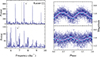 |
Fig. 6. As in Fig. 3, but for the Kazan observations. |
| In the text | |
|
Fig. 7. Results from a search for periods around the orbital one in TESS 23 light curves. Left panels: Periodograms of the observed light curves of the TESS-23a (top panel) and TESS-23b (bottom panel) observations in the frequency range of 6–8 d−1. The strongest peak corresponding to the negative (ν−) superhumps is labeled. The position of the νorb frequency is shown by the vertical dashed line. Right panels: TESS-23a (top panel) and TESS-23b (bottom panel) light curves folded with the period of the negative superhumps. The phase-binned light curves and their best sinusoid fits are also shown. |
| In the text | |
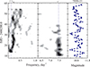 |
Fig. 8. As in Fig. 4, but for the TESS-23 observations. |
| In the text | |
|
Fig. 9. Results of searching long periods in all the investigated light curves. Left panels: Periodograms of the light curves obtained during all the observational intervals in the frequency range of 0.1–1.1 d−1. The vertical dashed lines show the positions of the frequencies corresponding to the expected periods of the nodal (left dashed lines) and apsidal (right dashed lines in the two upper panels) precessions of the tilted elliptical accretion disk. The periods corresponding to the two most stable peaks around periods 2.7–2.9 d and 1.8–1.9 d are marked. A peak corresponding to the observation duty cycle of 1 day is also visible in the middle panel. Right panels: Light curves folded with the most significant low-frequency periods. |
| In the text | |
|
Fig. 10. Time dependencies of the amplitudes of the photometric modulations with frequencies of lower than 1 d−1 found in the TESS-21 (top panels) and TESS-23 (bottom panel) data sets. |
| In the text | |
|
Fig. 11. Examples of searching for quasi-periodic oscillation in ground-based light curves. Top panels: Slidograms in the range of periods of 15–60 minutes during the nights 2023 January 7 (left panel) and 2022 August 1 (right panel). Middle panels: Corresponding periodograms in the same range of periods for the same nights. Bottom panels: Light curves folded with the most significant periods. |
| In the text | |
|
Fig. 12. Slidograms in the frequency range of 20–150 d−1 during the entire TESS-21 (left panel) and TESS-23 (right panel) observations. The vertical dashed lines show the positions of the break frequencies νc, 90 d−1 (TESS-21) and 72 d−1 (TESS-23). |
| In the text | |
|
Fig. 13. Total power spectra (gray curves) in log-log scale obtained using TESS-21 (top panel), Kazan-22 (middle panel), and TESS-23 (bottom panel) observations. The red circles show the averaged power spectra. The magenta lines show the power law with an exponent of −2, and the blue curves are the fits of the excess power spectra, represented by the formula (2) with the parameters A = 5, νc = 90 d−1, and γ = 2.2 (TESS-21), A = 2.7, νc = 90 d−1, and γ = 2.2 (Kazan-22), and A = 7, νc = 72 d−1, and γ = 2.2 (TESS-23). |
| In the text | |
|
Fig. 14. Geometry of the tilted disk precession. Here, n is a normal to the orbital plane, and the normal to the tilted accretion disk plane rotates around n with the period of the negative superhumps. |
| In the text | |
|
Fig. 15. Dependence of the amplitude of the system’s brightness change on the negative superhump period deficit ε− according to Table 3 in Bruch (2019). |
| In the text | |
Current usage metrics show cumulative count of Article Views (full-text article views including HTML views, PDF and ePub downloads, according to the available data) and Abstracts Views on Vision4Press platform.
Data correspond to usage on the plateform after 2015. The current usage metrics is available 48-96 hours after online publication and is updated daily on week days.
Initial download of the metrics may take a while.