| Issue |
A&A
Volume 690, October 2024
|
|
|---|---|---|
| Article Number | A288 | |
| Number of page(s) | 32 | |
| Section | Catalogs and data | |
| DOI | https://doi.org/10.1051/0004-6361/202347094 | |
| Published online | 17 October 2024 | |
JADES NIRSpec initial data release for the Hubble Ultra Deep Field
Redshifts and line fluxes of distant galaxies from the deepest JWST Cycle 1 NIRSpec multi-object spectroscopy
1
Department of Physics, University of Oxford,
Denys Wilkinson Building, Keble Road,
Oxford
OX1 3RH,
UK
2
Centre for Astrophysics Research, Department of Physics, Astronomy and Mathematics, University of Hertfordshire,
Hatfield
AL10 9AB,
UK
3
Cosmic Dawn Center (DAWN),
Copenhagen,
Denmark
4
Niels Bohr Institute, University of Copenhagen,
Jagtvej 128,
2200
Copenhagen,
Denmark
5
Scuola Normale Superiore,
Piazza dei Cavalieri 7,
56126
Pisa,
Italy
6
European Southern Observatory,
Karl-Schwarzschild-Strasse 2,
85748
Garching,
Germany
7
Kavli Institute for Cosmology, University of Cambridge,
Madingley Road,
Cambridge
CB3 0HA,
UK
8
Cavendish Laboratory – Astrophysics Group, University of Cambridge,
19 JJ Thomson Avenue,
Cambridge
CB3 0HE,
UK
9
Department of Physics and Astronomy, University College London,
Gower Street,
London
WC1E 6BT,
UK
10
NRC Herzberg,
5071 West Saanich Rd,
Victoria,
BC V9E 2E7,
Canada
11
Steward Observatory University of Arizona
933 N. Cherry Avenue
Tucson
AZ 85721,
USA
12
Astrophysics Research Institute, Liverpool John Moores University,
146 Brownlow Hill,
Liverpool
L3 5RF,
UK
13
Centro de Astrobiología (CAB), CSIC–INTA,
Cra. de Ajalvir Km. 4,
28850
Torrejón de Ardoz, Madrid,
Spain
14
Department of Physics and Astronomy, University of Manitoba,
Winnipeg
MB R3T 2N2,
Canada
15
European Space Agency (ESA), European Space Astronomy Centre (ESAC),
Camino Bajo del Castillo s/n, 28692 Villanueva de la Cañada, Madrid, Spain; European Space Agency, ESA/ESTEC, Keplerlaan 1,
2201 AZ
Noordwijk,
The Netherlands
16
Jodrell Bank Centre for Astrophysics, Department of Physics and Astronomy, School of Natural Sciences, The University of Manchester,
Manchester
M13 9PL,
UK
17
School of Physics, University of Melbourne,
Parkville
3010,
VIC,
Australia
18
ARC Centre of Excellence for All Sky Astrophysics in 3 Dimensions (ASTRO 3D),
Australia
19
Sorbonne Université, CNRS, UMR 7095, Institut d’Astrophysique de Paris,
98 bis bd Arago,
75014
Paris,
France
20
Max-Planck-Institut für Astronomie,
Königstuhl 17,
69117
Heidelberg,
Germany
21
Center for Astrophysics | Harvard & Smithsonian,
60 Garden St.,
Cambridge,
MA
02138,
USA
22
Department of Astronomy, University of Texas,
Austin,
TX
78712,
USA
23
ATG Europe for the European Space Agency, ESTEC,
Noordwijk,
The Netherlands
24
Department of Physics and Astronomy, The Johns Hopkins University,
3400 N. Charles St.,
Baltimore,
MD
21218,
USA
25
European Space Agency, Space Telescope Science Institute,
Baltimore,
MD,
USA
26
Department of Astronomy, University of Wisconsin-Madison,
475 N. Charter St.,
Madison,
WI
53706,
USA
27
Department for Astrophysical and Planetary Science, University of Colorado,
Boulder,
CO
80309,
USA
28
Observational Cosmology Laboratory, NASA Goddard Space Flight Center,
8800 Greenbelt Rd.,
Greenbelt,
MD,
USA
29
Max-Planck-Institut für Astronomie,
Königstuhl 17,
69117
Heidelberg,
Germany
30
Department of Astronomy and Astrophysics, University of California, Santa Cruz,
1156 High Street,
Santa Cruz,
CA
95064,
USA
31
NSF’s National Optical-Infrared Astronomy Research Laboratory,
950 North Cherry Avenue,
Tucson,
AZ
85719,
USA
★ Corresponding author; andy.bunker@physics.ox.ac.uk
Received:
4
June
2023
Accepted:
21
May
2024
We describe the NIRSpec component of the JWST Deep Extragalactic Survey (JADES), and provide deep spectroscopy of 253 sources targeted with the NIRSpec micro-shutter assembly in the Hubble Ultra Deep Field and surrounding GOODS-South. The multi-object spectra presented here are the deepest so far obtained with JWST, amounting to up to 28 hours in the low-dispersion (R~30–300) prism, and up to 7 hours in each of the three medium-resolution R ≈ 1000 gratings and one high-dispersion grating, G395H (R ≈ 2700). Our low-dispersion and medium-dispersion spectra cover the wavelength range 0.6–5.3 μm. We describe the selection of the spectroscopic targets, the strategy for the allocation of targets to micro-shutters, and the design of the observations. We present the public release of the reduced 2D and 1D spectra, and a description of the reduction and calibration process. We measure spectroscopic redshifts for 178 of the objects targeted extending up to z = 13.2. We present a catalogue of all emission lines detected at S/N > 5, and our redshift determinations for the targets. Combined with the first JADES NIRCam data release, these public JADES spectroscopic and imaging datasets provide a new foundation for discoveries of the infrared universe by the worldwide scientific community.
Key words: instrumentation: spectrographs / surveys / galaxies: evolution / galaxies: high-redshift
© The Authors 2024
 Open Access article, published by EDP Sciences, under the terms of the Creative Commons Attribution License (https://creativecommons.org/licenses/by/4.0), which permits unrestricted use, distribution, and reproduction in any medium, provided the original work is properly cited.
This article is published in open access under the Subscribe to Open model. Subscribe to A&A to support open access publication.
1 Introduction
JWST (Gardner et al. 2023) is the largest programme in astrophysics to date, and is far more than simply the successor to the Hubble Space Telescope (HST). As well as having seven times the collecting area of HST, JWST operates over a wider range of wavelengths (0.6–25 μm) in a lower-background environment (at L2), making it orders of magnitude more sensitive than previous observatories. One of the major goals of the JWST mission is to study the formation and evolution of galaxies, in particular in the early universe through observations of high redshift galaxies.
The JWST Advanced Deep Extragalactic Survey (JADES, Bunker et al. 2020; Rieke 2020; Eisenstein et al. 2023) is the largest Cycle 1 programme aiming to study galaxy evolution out to the highest redshifts. JADES is a coordinated survey designed and executed by the NIRSpec and NIRCam Guaranteed Time Observation (GTO) teams. It provides NIRCam and MIRI imaging as well as NIRSpec spectroscopy over two fields. An important aspect of JADES is the assembly of a large data set of spectroscopic observations spanning from cosmic noon to within the epoch of reionization, enabling confirmation of high-redshift candidates, accurate redshift measurements, and unprecedented constraints on the physical conditions in distant galaxies. With such spectroscopy, we can explore the mass-metallicity relation, dust attenuation, star formation rates and star formation histories in galaxies, as well as ionization parameters, ionizing photon escape fraction, and the presence of any active galactic nuclei. Spectroscopy is also key to understanding the physical states of the interstellar, circumgalactic and intergalactic media, and their evolution with cosmic time. Crucially, assembling this data set is enabled by the new multi-object spectroscopy (MOS) capabilities of JWST with the near-infrared spectrograph (NIRSpec; Jakobsen et al. 2022).
NIRSpec operates in the range 0.6–5.3 μm, and has three spectral resolutions: a low-dispersion prism (R ≈ 30–300) which captures all the wavelength range with a single exposure, and medium- and high-resolution gratings (R ≈ 1000 and R ≈ 2700) which use three bands to cover the wavelength range. One unique feature of this spectrograph is its use of a micro-shutter assembly (MSA), developed specifically for NIRSpec to enable multi-object spectroscopy of hundreds of objects at once over a ![$\[3^\prime_\cdot6 \times 3^\prime_\cdot4\]$](/articles/aa/full_html/2024/10/aa47094-23/aa47094-23-eq1.png) field of view (Ferruit et al. 2022).
field of view (Ferruit et al. 2022).
As described in Eisenstein et al. (2023), JADES has Deep and Medium tiers, where the Medium tier adds area to capture rarer objects, while the Deep tier allows for searches of the faintest, and most distant galaxies. The survey covers two fields with huge legacy data sets thanks to the Great Observatories Origins Deep Survey (GOODS Dickinson et al. 2003; Giavalisco et al. 2004), GOODS-South and GOODS-North. As well as the multi-wavelength efforts of the original GOODS survey, there have been extensive observing efforts in the same area, including, but not limited to, the CANDELS survey with Hubble (Cosmic Assebly Near-Infrared Deep Extragalactic Legacy Survey, Grogin et al. 2011; Koekemoer et al. 2011) and the GREATS survey with Spitzer (GOODS Re-ionization Era wide-Area Treasury from Spitzer, Stefanon et al. 2021). In particular the GOODS-South field includes the region of the sky with the deepest Hubble images ever taken, the Hubble Ultra Deep Field (HUDF, Beckwith et al. 2006; Bouwens et al. 2010; Ellis et al. 2013), where we focus the Deep portion of our survey. The Medium tier adds area with observations in GOODS-North, and the extended GOODS-South field, predominantly within the footprint of the CANDELS data.
In this paper, we present our deep spectroscopy of targets in the HUDF and surrounding GOODS-South field and outline our target selection strategy. We release the raw data and make our reduced data products available to the community1, and in a companion paper (Rieke et al. 2023) we present the complementary JADES NIRCam imaging of the HUDF. From the prism and medium-dispersion R ≈ 1000 spectra we derive redshifts and fluxes of prominent emission lines. The data from the single high-dispersion grating used (G395H, R ≈ 2700) also forms part of this data release, but we do not perform detailed on this analysis in this paper.
The structure of this paper is as follows. Section 2 describes how potential spectroscopic targets were selected from imaging data (primarily a combination of JADES NIRCam and HST), and how these were allocated to different priority classes so that the NIRSpec MSA configuration could be optimised for our science goals. The NIRSpec observations are described in Section 3 and the data processing is outlined in Section 4. In Section 5 we present our redshift measurements, and detected emission line fluxes of individual galaxies. Our conclusions are in Section 6. Throughout this work, we assume the Planck 2018 cosmology (Planck Collaboration VI 2020) and the AB magnitude system (Oke & Gunn 1983).
2 Targets
JADES observations take NIRCam imaging and NIRSpec spectroscopy in parallel. As the survey progresses, JADES aims to leverage NIRCam photometry to select targets for later NIRSpec observations where possible, as this will enable the identification of the highest-redshift objects and facilitates near mass-limited samples at lower redshifts. However, for many of our early observations, we take spectroscopy in regions which have not yet been imaged by NIRCam.
In the initial planning phase, the Deep tier presented here was to be observed prior to NIRCam imaging and hence would comprise only targets previously identified (mostly from HST imaging). However, scheduling changes meant that we ended up having NIRCam data available shortly before our final MSA configuration needed to be set2. This unforeseen opportunity was exploited scientifically to refine the target selection by making use of the additional JADES photometry from NIRCam images, with observations completed 16 days before the NIRSpec observations. Thus, our selected targets represent a NIRCam-based selection, supplemented with some HST-based targets compiled from the literature. We note that the NIRCam images available when drawing up our target list did not cover the full region of the NIRSpec MSA (see Figure 1).
We used NIRCam data taken between 29th September and the 5th October 2022 described in Rieke et al. (2023), which added nine photometric bands, potentially improving photometric redshifts over previous HST-based studies as well as identifying HST-dark sources. We used a very early reduction of the data and describe the limitations of this in Appendix B. We measured the HST and NIRCam photometry using ![$\[0^{\prime\prime}_\cdot3\]$](/articles/aa/full_html/2024/10/aa47094-23/aa47094-23-eq2.png) -arcsec diameter apertures and applying aperture corrections for each filter appropriate for compact sources. We estimated photometric redshifts from two different SED-fitting codes with very different template sets and underlying assumptions, EAZY (Brammer et al. 2008) and BEAGLE (Chevallard & Charlot 2016), and these were used in our target selection.
-arcsec diameter apertures and applying aperture corrections for each filter appropriate for compact sources. We estimated photometric redshifts from two different SED-fitting codes with very different template sets and underlying assumptions, EAZY (Brammer et al. 2008) and BEAGLE (Chevallard & Charlot 2016), and these were used in our target selection.
In this Section, we first describe our over-arching prioritisation system for allocating targets for spectroscopy. We then describe the assembly of these NIRCam- and HST-based catalogues, which formed the source material for our target allocation.
2.1 Priority class system
The target selection for the NIRSpec MOS observations was designed to prioritise rare targets, either at high redshift, or with low number density, while building up a statistical sample spanning from cosmic noon to within the epoch of reionization. This was achieved by sorting the potential targets into a limited number of priority classes and employing the NIRSpec team’s eMPT software suite (Bonaventura et al. 2023) to optimise the placement of targets within each class in sequence on the MSA. The priority class criteria employed are presented in Table 1. The science goals for the JADES survey as a whole are diverse (Section 1, see also Eisenstein et al. 2023), and the first deep pointings presented here represent the initial step in building up the entire sample.
We emphasise that the JADES NIRSpec survey does not employ a single selection function, but within each priority class there is a well defined set of criteria. The highest priority targets (Class 1) are used to set and optimise the NIRSpec pointing centres (see Section 2.3) and are the bright, robust highest redshift candidates (z > 8.5). Classes 2 and 3 allow for less robust candidates and fainter candidates, respectively, at similarly high redshifts. Progressing down the priority classes predominantly represents a progression in decreasing redshift, as the number counts then increase. A notable departure from this is Class 5 in which we include bright objects to achieve a few high signal-to-noise continuum spectra per pointing.
In Class 4, we aim to target galaxies in the redshift interval 5.7 < z < 8.5 which are expected to have sufficiently bright rest-frame optical emission lines to enable emission line ratio work and exploration of interstellar medium (ISM) conditions (Cameron et al. 2023; Curti et al. 2024). Our goal is to achieve S /N > 25 in the Hα line (available at z < 7) or, when not available (i.e. z > 7), [O III] λ5007. This would gives an expected S /N ≈ 8 or more for the Hβ line, and the resulting uncertainty of 10–15% on the Balmer decrement, f(Hα)/f(Hβ), allows for an estimate of the attenuation due to dust (e.g. Sandles et al. 2023). To achieve these target emission line fluxes in Class 4, we select on the rest-frame UV magnitude around 1500 Å. At z ≈ 6, a galaxy with a star formation rate of 2.5 M⊙ yr−1 has a magnitude in the F115W filter of AB = 27.5 for the rest-UV longward of the Lyman-α break (assuming a Salpeter 1955 initial mass function and no dust extinction), and an expected Hα flux of 3 × 10⁻¹⁹ erg cm−2 s−1 at 4.5 μm (adopting the Kennicutt 1998 conversion from star formation rate to Hα flux). This should be detectable at S/N = 25 in the prism spectroscopy of the Deep tier of JADES (duration ≈ 100 ksec), using the STScI Exposure Time Calculator3. Hence for Class 4 we adopt a magnitude cut of AB = 27.5 in the broad-band filters just above the Lyman-α break. Fainter targets in the same redshift interval appear in Class 6.
Class 7 represents the statistical sample spanning 1.5 < z < 5.7, which will be built up over multiple tiers, spanning from cosmic noon to the epoch of reionization. Within Class 7, we paid particular attention to placing unusual objects first before the more common star-forming galaxy population. Specifically, galaxies which exhibited colours in the rest-frame UVJ colour-colour plane consistent with being passive or quenched galaxies were identified following the criteria for specific star formation rate (sSFR), log(sSFR/yr−1) < −9.5 given in Leja et al. (2019). We also prioritised ALMA sources which had a match to sources in the HST or NIRCam images (e.g. Aravena et al. 2016; Decarli et al. 2016; Rujopakarn et al. 2016; Dunlop et al. 2017; Franco et al. 2018; Yamaguchi et al. 2019; Hodge et al. 2013), along with AGN including those selected from the IR, from variability, or from X-ray selection with an optical/near-IR counterpart (Alonso-Herrero et al. 2006; Castelló-Mor et al. 2013; Del Moro et al. 2016; Luo et al. 2011, 2017; Sarajedini et al. 2011; Treister et al. 2006, 2009b,a; Young et al. 2012).
Any unused areas on the MSA following the placement of sources in Classes 1–7 (described above) were filled with very low priority targets in Class 8 and 9, which comprised: fainter targets which did not pass the brightness to be in Class 7; targets at lower redshifts than z ≈ 1.5; and targets for which the astrometry was unreliable. Blank sky shutters were also added.
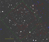 |
Fig. 1 Field layout of the NIRSpec Deep-HST observations presented in this paper. The green rectange is the region covered by the original HST/ACS Hubble Ultra Deep Field. The red rectangle is the smaller area covered in the Ultra Deep HST/WFC 3 imaging. The background image is the NIRCam F200W from JADES, except for the region to the right of the blue line which has not yet been observed by NIRCam; we show in this region the HST/WFC 3 from GOODS-South/CANDELS in blue. The short red lines denote the five-shutter ( |
![$\[2^{\prime\prime}_\cdot6\]$](/articles/aa/full_html/2024/10/aa47094-23/aa47094-23-eq3.png)
Target prioritisation categories.
2.2 Establishing input catalogue of possible spectroscopic targets
The Hubble Ultra Deep Field (HUDF) and surrounding GOODS-South are very well studied fields. To provide an input target list for potential observation with the NIRSpec MSA, we compiled a large list of galaxies from the literature, which we cross-matched with our NIRCam-derived catalogues after first correcting the coordinates of the literature sources onto the same Gaia DR2 astrometric frame (see Appendix A), leveraging the CHArGE re-reduction of the GOODS-S HST imaging which has been registered to the Gaia DR2 astrometric frame (Kokorev et al. 2022; Brammer 2023)4. Where no match to an HST-detected object was identified within ![$\[0^{\prime\prime}_\cdot3\]$](/articles/aa/full_html/2024/10/aa47094-23/aa47094-23-eq6.png) with the NIRCam-based catalogue (with co-ordinates defined as target centres), the target catalogue was supplemented with the HST-detected object. In regions of MSA footprint with no NIRCam coverage, all objects are taken from the HST-based catalogues. We later impose selection criteria to populate the various priority classes which dictated the allocation of observed sources to the MSA micro-shutters. The priority classes for each object eventually observed are presented in Table F.1, where we list the final priorities allocated on the basis of NIRCam photometry (where available), and we also give the initial priority allocations on the basis of HST data alone.
with the NIRCam-based catalogue (with co-ordinates defined as target centres), the target catalogue was supplemented with the HST-detected object. In regions of MSA footprint with no NIRCam coverage, all objects are taken from the HST-based catalogues. We later impose selection criteria to populate the various priority classes which dictated the allocation of observed sources to the MSA micro-shutters. The priority classes for each object eventually observed are presented in Table F.1, where we list the final priorities allocated on the basis of NIRCam photometry (where available), and we also give the initial priority allocations on the basis of HST data alone.
A main driver of the JADES survey is to observe the highest redshift targets, for which we compiled a sample of galaxies which had been identified as z > 5.6 candidates by one or more studies in the literature, or from our NIRCam+HST analysis. The lower end of this redshift range corresponds to where the i′-band drop-out technique using the HST/ACS filter set becomes effective. The list of galaxies compiled from the literature includes any studies that have previously selected z ≳ 6 candidates based on the Lyman break technique and/or photometric redshifts (Bunker et al. 2004; Yan & Windhorst 2004; Oesch et al. 2010, 2013; Lorenzoni et al. 2011, 2013; Yan et al. 2010; Ellis et al. 2013; McLure et al. 2013; Schenker et al. 2013; Bouwens et al. 2015, 2021; Finkelstein et al. 2015; Harikane et al. 2016). The sample from the literature was largely based on Lyman-break drop-out selection (e.g. Bunker et al. 2004; Bouwens et al. 2015) although some are more generally based on photometric redshifts (e.g. Finkelstein et al. 2015). We cross-matched different samples in the literature which present high redshift candidates, and we note that while many galaxies were in common (using a matching tolerance of ![$\[0^{\prime\prime}_\cdot2\]$](/articles/aa/full_html/2024/10/aa47094-23/aa47094-23-eq7.png) ), there was a significant fraction which appeared in only one selection. This may be due to those papers using earlier reductions of HST data, perhaps not including all the data now available, or slightly different colour cuts, S /N thresholds, and photometric aperture choices by the various research groups. Hence, to refine this selection of potential high-redshift targets, we inspected all the z > 5.6 candidates from the literature. We used a slightly lower redshift cut for this inspection of candidates than ultimately adopted for Classes 4 and 6 (z > 5.7, Table 1) so as to allow slight changes in photometric redshift due to our remeasured photometry. For each z > 5.6 candidate, we re-measured the aperture photometry from the HST images (with
), there was a significant fraction which appeared in only one selection. This may be due to those papers using earlier reductions of HST data, perhaps not including all the data now available, or slightly different colour cuts, S /N thresholds, and photometric aperture choices by the various research groups. Hence, to refine this selection of potential high-redshift targets, we inspected all the z > 5.6 candidates from the literature. We used a slightly lower redshift cut for this inspection of candidates than ultimately adopted for Classes 4 and 6 (z > 5.7, Table 1) so as to allow slight changes in photometric redshift due to our remeasured photometry. For each z > 5.6 candidate, we re-measured the aperture photometry from the HST images (with ![$\[0^{\prime\prime}_\cdot36\]$](/articles/aa/full_html/2024/10/aa47094-23/aa47094-23-eq8.png) -diameter apertures and appropriate aperture corrections) and ran photometric redshift fits with EAZY (Brammer et al. 2008) and BEAGLE (Chevallard & Charlot 2016). For those galaxies which also appeared in our NIRCam-based catalogue, we also calculated the photometric redshift including both the NIRCam and HST photometry.
-diameter apertures and appropriate aperture corrections) and ran photometric redshift fits with EAZY (Brammer et al. 2008) and BEAGLE (Chevallard & Charlot 2016). For those galaxies which also appeared in our NIRCam-based catalogue, we also calculated the photometric redshift including both the NIRCam and HST photometry.
We also visually inspected the HST images (and NIRCam images where available) in all wavebands, using a co-addition of all the HST data taken in the GOODS-South field from the Hubble Legacy Field v2.0 images (Whitaker et al. 2019; Illingworth et al. 2016), which goes deeper than many of the images used in the past to construct the early catalogues of Lyman break galaxies. For the sources selected from NIRCam photometry, we also removed spurious high redshift candidates due to artifacts and deblending issues.
We retained only the most robust candidates in our highest priority classes, those which were clearly detected at longer wavelengths, had a strong spectral break and were undetected at short wavelengths, and where the photometric redshifts strongly favoured a high redshift solution. Some objects were either only faintly detected or had spectral energy distributions where the photometric redshift was unclear (with both high and low redshift solutions possible). These were placed in a class for more marginal targets, which were allocated at lower priority than the more robust candidate high-redshift galaxies. In the case of the highest redshifts (zphot > 8.5) from the previous literature, the most robust candidates with HST F160W magnitudes brighter than AB = 29 were placed in the top priority ‘Class 1’ (Table 1), with those judged to be less robust placed in Class 2. From our NIRCam-based selection, we added two targets not appearing in the literature to Class 1 which had robust photometric redshifts z > 9 and were brighter than AB = 29.5 mag in filters just longward of the putative Lyman-α break, and a further two NIRCam-selected targets which were judged to be less robust were added to Class 2. Galaxies with zphot > 8.5 and fainter than F160W AB = 29 in the literature-based selection appear in Class 3.
Galaxies with redshifts in the interval 5.7 < z < 8.5 span the epoch of reionization and are also potentially selected by the Lyman-break technique using drop-outs in the F775W, F850LP and F105W filters on HST. For these targets, we impose a magnitude cut on the broad-band filter longward of the Lyman-α break, sampling the rest-frame UV (a proxy for star formation). Those galaxies brighter than AB = 27.5 in that filter were allocated to Class 4 (with this magnitude cut justified in Section 2.1), with less robust candidates and slightly fainter galaxies (27.5 < AB < 29) in Class 6.1. Candidates fainter than AB = 29 appear in Class 6.2. Some objects were up-weighted in this visual inspection exercise from Class 6 to Class 4 if they showed signs of strong line emission in the NIRCam photometry (<20%). Our input sample, after visual inspection and photometric checks, comprised about 300 galaxies at z > 5.7 within the total NIR-Spec MSA footprint. There were other cases (about 5% of the sample drawn from the literature) where we identified targets which seem to have flux below the putative Lyman-α break, and these were demoted to lower redshift classes based on the our revised photometric redshifts (including the NIRCam photometry where available). A number of high-redshift candidates from the literature were essentially undetected in the full co-added HST imaging, and these were removed from our sample (about 20%, but we note that many of these would not have passed the magnitude cuts to place them in our very highest priority classes).
Galaxies with photometric redshifts below z = 5.7 formed our lower-priority classes, in particular Class 5 (bright objects), and Class 7 (a magnitude-limited sample prioritised in redshift slices). When assigning priorities in Class 7, we used the opportunity to base the magnitude limit of AB = 29 mag on the longest wavelength NIRCam filter available (F444W), to make the selection as close to a mass-selected sample as possible, and to homogenise the selection with that planned for other tiers of JADES. Where NIRCam imaging was not available (or a literature source did not have a match in our NIRCam catalogue), we imposed a magnitude cut in HST/WFC 3 F160W of AB = 29, as this H-band filter is the reddest available HST data. This HST photometry for each galaxy was drawn from the latest available catalogue in which it appeared out of: Whitaker et al. (2019), Rafelski et al. (2015), Skelton et al. (2014) or Guo et al. (2013). If the source did not appear in any of these large catalogues, then we adopted the HST H-mag from the discovery paper if available (e.g. Lyman break catalogues) or we remeasured the photometry.
In Class 7, photometric redshifts are used to assign objects to four different redshift bins, with the smaller number of objects in the higher redshift slice 4.5 < z < 5.7 being allocated to MSA shutters before the next slice (3.5 < z < 4.5) and then those with 2.5 < z < 3.5 and finally 1.5 < z < 2.5. In the MSA target allocation in Class 7, we first placed the unusual targets (quiescent galaxies, AGN and ALMA sources) descending through the four redshift bins in order (sub-classes 7.1–7.4) before then placing shutters on the more common star-forming galaxies, again working down the four redshifts bins in turn to allocate targets. Where available, the photometric redshifts were drawn from the high-redshift catalogues of Bouwens et al. (2021), Finkelstein et al. (2015) or Bouwens et al. (2015), which generally utilised the Lyman break in HST filters extending to the UV. We supplemented Class 7 with photometric redshifts from the UVUDF survey (Rafelski et al. 2015), or, if unavailable, from the 3DHST survey (Brammer et al. 2012; Skelton et al. 2014), which in particular extended to lower redshifts than the Lyman break selected catalogues. For some lower redshift objects, the additional NIRCam photometry was not guaranteed to improve the photometric redshifts due to the small aperture used compared to the size of the objects, and the differences in point spread function (PSF). We therefore only replaced the HST-derived photometric redshift with the HST+NIRCam-derived photometric redshift when the BEAGLE and EAZY photometric redshifts agreed. Specifically, the redshift bin was assigned first using the HST-based photometric redshift (where available). This was then adjusted only if the range between the EAZY and BEAGLE (primary or secondary redshift solution) 95% credible regions overlapped, or the redshift solutions agreed within Δz = 0.1. As with Classes 1–6, all the Class 7 sources were visually inspected on the HST and NIRCam images, and a few eliminated as being unreliable.
2.3 Target assignment
The NIRSpec multi-object spectroscopic observations presented in this paper were carried out in MOS mode with the MSA (Ferruit et al. 2022) with NIRCam operating in parallel. The MSA configurations employed were designed using the NIRSpec GTO team’s so-called eMPT software suite (Bonaventura et al. 2023), and then imported into the STScI Astronomers Proposal Tool (APT) for execution. For a given choice of disperser and assigned roll angle, the eMPT is capable of identifying the pointings of the MSA on the sky that capture the largest possible number of high priority targets whose images fall within the open areas of operational shutters to a specified accuracy without their spectra overlapping on the detector. Three shutter tall slitlets were assigned to each target, and the telescope was nodded by one shutter facet (529 mas) along the spatial direction such that the targets were observed in each shutter in sequence. An ‘acceptance zone’ spanning 184 mas in the dispersion direction and 445 mas in the spatial direction was employed throughout, corresponding to the full open area of a shutter with ≃9 mas shaved off the edges. This was to prevent targets leaving the open shutter areas during any of the nods due to differential optical distortion arising in the telescope and NIRSpec optics. For all targets, only shutters whose low resolution prism spectra avoid truncation by the gap between the two detector arrays of NIRSpec (Jakobsen et al. 2022; Ferruit et al. 2022) were employed.
As described in Bonaventura et al. (2023), the eMPT approach to designing the MSA masks starts by exercising its so-called ‘initial pointing algorithm’ (IPA) module. This identifies the ensemble of candidate pointings within a specified range of the nominal pointing that provide the largest possible coverage of the targets designated as Priority Class 1 in the input catalogue at the roll angle assigned to the observation. Other eMPT modules are then employed to fill up the remainder of the MSA mask at each pointing with additional targets in decreasing order of scientific priority. For the observations presented here, three separate ‘dithered’ pointings were planned with the goal of smoothing out detector defects in the dispersed spectra beyond that achieved by the three nods performed at each pointing. For the highest priority targets the objective was to achieve the largest possible total exposure time by observing these targets at all three dithers, while for the brighter lower priority targets the desire was to observe as many targets as possible, especially considering that these targets are placed on the MSA last and therefore become progressively more difficult to accommodate. For any given trial of three pointings drawn from the set of all optimal Priority Class 1 covering pointings identified by the IPA module, the eMPT distinguishes between targets that can be observed at all three pointings, in only two of the pointings, and in only a single pointing, and gives the user complete control over the order in which targets in each subset are placed on the MSA. This process is carried out for all candidate triple pointings that constitute reasonable dithers of the spectra on the detector, and the triple pointing achieving the best overall target coverage was selected as the final one.
Another important consideration when using the MSA is to avoid targets being contaminated by the unintended light from nearby targets entering any of the (nodded) slitlets. The eMPT automatically eliminates such targets in a ‘point source’ manner based on the input catalogue, but since the contamination due to extended sources is difficult to automate, the candidate MSA masks produced by the eMPT were subjected to a final visual inspection. Remaining undesirable targets were flagged and subsequently removed from the MSA masks. However, since the removal of a higher priority target can significantly change the placement of all lower priority targets that are placed after it, rather than start the process again from scratch, bespoke software was employed that allowed the process to converge after one or two iterations by optimally filling the gaps in the MSA opened up by removed contaminated targets with other non-overlapping ones, while leaving all others in place.
The grating exposures taken at each pointing employed as the starting point the same MSA masks as the prism exposures, but were modified using bespoke software to protect the grating spectra of the first five priority class targets by closing all shutters containing lower priority targets whose spectra collided with those of the higher priority targets.
Through the above process, prism spectra of a total of 253 unique objects were obtained in the three pointings and series of exposures described in this paper. Of these, 27% were observed in all three pointings, 24% in two pointings, and 49% in a single pointing. The three pointings cover 145, 155 and 149 individual prism targets each. In comparison, the grating observations cover a total of 198 unique targets, of which 28% are observed at three pointings, 21% at two pointings and 51% in a single pointing. The three grating pointings cover 119, 121 and 111 individual targets each.
In practice, the late addition of high priority NIRCam sources, and re-prioritisation of the catalogue (see Section 2.2) were incorporated without being able to re-optimise the pointings themselves. As a consequence, only four of the six highest priority targets in Table F.1 were observed in three dithers as opposed to all of them as would have been the case if the pointing could have been tweaked. One of the added Priority 1 NIRCam targets (ID 2773) was observed in two pointings and a second one (ID 17400) in only a single pointing.
3 Observations
The NIRSpec MSA observations of JADES Deep/HST were taken on UT 21–25 October 2022 as the JWST Program ID: 1210 (PI: N. Lützgendorf). The observations were split into three visits, which differed in their pointings by < 1 arcsec and employed separate MSA masks (see Section 2.3) but identical exposure sequences. The three pointings were selected such that they shift the spectra on the detector by a sufficient amount in order to smooth out detector defects; one shutter (268 mas or 2.6 pixels) in the dispersion direction plus one shutter (529 mas or 5.0 pixels) in the spatial direction for the second pointing, and three shutters (804 mas or 7.8 pixels) in the dispersion direction for the third pointing.
At each pointing we took observations with the low-resolution prism and four grating/filter combinations (G140M/F070LP, G235M/F170LP, G395M/F290LP and G395H/F290LP). We used the NRSIRS2 readout pattern (Rauscher et al. 2017) with 19 groups for an integration time of 1400 seconds, with two integrations per exposure. The MSA configurations opened three adjacent shutters for each target and the targets were ‘nodded’ between these shutters (perpendicular to the dispersion direction) with an exposure at each position. For the prism only, this sequence was repeated four times to obtain very deep observations. At each one of the three pointings the total integration time (number of exposures) was 33.6 ks (24) for the prism and 8.4 ks (6) for each grating. Thus the sources observed in all three pointings attained total integration time of 100 ks for the prism and 25 ks for each grating.
4 Data processing
In processing this data, the NIRSpec GTO Team used a custom pipeline derived from the pipeline originally developed by the ESA NIRSpec Science Operations Team (SOT) described in section 4.3 of Ferruit et al. (2022) and based on the workflow and algorithms described in Alves de Oliveira et al. (2018). This custom pipeline will be presented in a future paper (Carniani et al., in prep.). We briefly describe here the main data reduction steps. The two NIRSpec detectors were read non-destructively multiple times using the NRSIRS2 readout mode. The master bias frame and dark current were subtracted, and we also corrected artefacts such as snowballs (Ferruit et al. 2022; Giardino et al. 2019). For each exposure we fit the slope (i.e. the count rate) for each pixel, identifying and removing jumps due to cosmic ray strikes, and flagging when saturation occurred. We background-subtracted the 2D spectrum in each shutter by taking the average of the two other exposures in the three-nod pattern. In some cases of spatially-extended objects, or those falling close to one end of a shutter, we excluded the adjacent shutter containing light from the target object (or in some cases a contaminating source) from the background subtraction. We note that very extended sources (a small minority of our targets) may be prone to some self-subtraction using this local background subtraction approach.
The individual 2D spectra from each shutter were then flat fielded and corrected for illumination by the spectrograph optics and the wavelength-dependent throughput of the dispersing element. The wavelength and flux calibration was then applied, with each pixel of the 2D spectrum having an associated wavelength and distance along the shutter, accounting for the slight tilt of the shutters relative to the dispersion direction, along with optical distortions. At each stage of the data reduction process we also propagated noise and data quality arrays.
The position of the object within the micro-shutter along the dispersion direction was also taken into account when applying the wavelength calibration – many of our targets are compact (Figure 2 and Figure 3) with intrinsic sizes smaller than the ![$\[0^{\prime\prime}_\cdot2\]$](/articles/aa/full_html/2024/10/aa47094-23/aa47094-23-eq9.png) shutter width, so making wrong assumptions about the slit being uniformly illuminated or that each object is well centered would lead to wavelength offsets. We applied a path-loss correction to account for flux falling outside the micro-shutter; given the large wavelength range covered by NIRSpec (0.6 < λ < 5.3 μm) it was critical to account for the considerable PSF variation with wavelength. We took into account the position of the object within the micro-shutter (see the “intra-shutter offset” columns in Table F.1), and calculated the slit loss as a function of wavelength for a point source at this location; this was a reasonable approximation for many of our targets which are often compact (Figure 2), particularly at high redshift and also potentially for the star-forming regions giving rise to emission lines within more extended galaxies.
shutter width, so making wrong assumptions about the slit being uniformly illuminated or that each object is well centered would lead to wavelength offsets. We applied a path-loss correction to account for flux falling outside the micro-shutter; given the large wavelength range covered by NIRSpec (0.6 < λ < 5.3 μm) it was critical to account for the considerable PSF variation with wavelength. We took into account the position of the object within the micro-shutter (see the “intra-shutter offset” columns in Table F.1), and calculated the slit loss as a function of wavelength for a point source at this location; this was a reasonable approximation for many of our targets which are often compact (Figure 2), particularly at high redshift and also potentially for the star-forming regions giving rise to emission lines within more extended galaxies.
The spectra are curved on the detector due to optical distortions, and we rectify the 2D spectrum (transforming such that the wavelength and distance along the microshutter in the cross-dispersion direction lie along the x and y axes respectively), re-sampling the 2D spectrum onto a finer wavelength grid in the process. For the gratings, the re-sampled pixel scale was 6.36 Å, 10.68 Å and 17.95 Å for the G140M, G235M and G395M gratings, respectively. For the prism, where the resolving power varies in a non linear way between R ≈ 30–330 (Jakobsen et al. 2022), we used an irregularly-gridded wavelength sampling with intervals between 26–122 Å, with the coarsest sampling (largest wavelength interval per pixel) around 1.5 μm where the resolving power is at its lowest. The 1D spectra for the three nod positions from each of the (up to) three pointings were then combined by a weighted average into a single 1D spectrum for each target, masking pixels previously flagged as bad in the data quality files, and rejecting outliers using a sigma clipping algorithm. We also separately combined all the 2D spectra for each target from the different nods and pointings, although the 1D combined spectrum comes from a combination of the 1D individual spectra rather than an extraction of the combined 2D spectrum. The resulting 1D and 2D spectra reduced data products for all targets are made available as part of this data release, along with the raw data. Example spectra covering a range of redshifts are shown in Appendix E (Figures E.1–E.10).
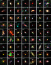 |
Fig. 2 Overlay of target shutter positions onto the images, with the illuminated shutter regions outlined ( |
![$\[0^{\prime\prime}_\cdot46 \times 0^{\prime\prime}_\cdot20\]$](/articles/aa/full_html/2024/10/aa47094-23/aa47094-23-eq10.png)
![$\[1^{\prime\prime}_\cdot0\]$](/articles/aa/full_html/2024/10/aa47094-23/aa47094-23-eq11.png)
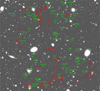 |
Fig. 3 One of the four MSA quadrants (Q3), showing allocation of micro-shutters to targets. The other quadrants are shown in Appendix D. Those shutters in green are covered by both the grating configurations and the low-dispersion prism. The red shutters are open only in the prism observations, as they would lead to overlapping spectra for our high priority targets in the grating configuration. Three micro-shutters are opened for each target, but the nodding by ±1 shutter means that spectra are obtained over the areas covered by five shutters (including background) which are displayed. The field displayed is the NIRCam F200W image, and is 1.8 arcmin on a side. North is up and East is to the left. Shutters with the prefix ‘B’ are empty sky background. |
5 Redshift determination and emission line fluxes
In this section, we report spectroscopic redshifts and emission line fluxes determined from our spectroscopic observations, and assess the success rate of our priority class system for target selection.
5.1 Visual inspection and emission line fitting
The 1D and 2D spectra of all spectral configurations were visually inspected as a first pass on the redshift determination. The SED fitting code BAGPIPES (Carnall et al. 2018, 2019) was run on the 1D Prism/CLEAR spectra and the redshifts arising from this fitting were used a starting point for the inspection, but ultimately the assessment of the human inspector would overrule this value if necessary. In many cases, several clear emission lines were observed and the redshifts were unambiguous. Sometimes spectral breaks were visible, most notably the Lyman-α break (e.g. Curtis-Lake et al. 2023; Looser et al. 2024), and sometimes the Balmer break or 4000 Å break. In fainter targets, the S /N of individual features were sometimes low, but the coincidence of more than one of these led to a tentative redshift.
We then performed emission line fitting to further refine the redshifts, and obtain measurements of the fluxes of significant emission lines. For the R ≈ 1000 grating data, the continuum was typically only marginally detected and we subtracted this by fitting a spline to the spectrum after masking out any regions which could be contaminated by prominent emission lines. We then performed a single-component Gaussian fit to each line individually, allowing the flux, redshift and line-width to vary independently. In the case of unresolved doublets, such as [O II] λλ3726, 3729, we simply fit the entire doublet as a single component. In the case of Hα and [N II] λ6583, although these lines are never blended in our R ≈ 1000 grating data, these lines were fit simultaneously and had their line centroids fixed relative to one another. The line flux was obtained as the integrated area under the best-fit Gaussian, and the formal uncertainty on this Gaussian fit was taken as the noise on the line flux. We retained only emission lines which were measured with S/N > 5, and visually inspected each fit to ensure the measurement was robust. The emission line fluxes arising from this are reported in Table F.2. We note that there were two cases (ID 10013704 and ID 8083) where a broad component under Hα meant that a single component fit was not appropriate. In these cases, the reported Hα flux is obtained by integrating the whole line between the zero-power points in the spectrum.
In the case of the Prism/CLEAR data, the much lower spectral resolution (R ≈ 30–300) means that blending of emission lines is much more common in these data. Furthermore, which emission lines are blended changes with galaxy redshift due to the wavelength-dependent nature of the resolution. For this reason, although the approach to emission line fitting on the Prism/CLEAR spectra largely followed the same process as described above for the R ≈ 1000 mode, some redshift-dependent modifications were implemented. As such, which line fluxes are reported as blends changes with redshift. At all redshifts for the prism data, Hα+[N II] was fit as a single component, as were close doublets such as [O II] λλ3726, 3729 and [S II] λλ6716, 6731. The flux of Hα+[N II] and [S II] λλ6716, 6731 were fit for simultaneously, with fixed centroids. In all cases, the fit to Hβ and [O III] λλ4959, 5007 was performed simultaneously with the centroids fixed relative to one another. Above z > 5.3, the fluxes of all three components were fit (and reported) independently. At lower redshifts, the ratio of [O III] λ5007/λ4959 was fixed to 2.98, but the Hβ flux could still vary independently. Between 2 < z < 5.3, we report the flux of the [O III] λλ4959, 5007 as a blend. For the [O III] λ4363 and Hγ complex, above z > 7.5, the resolution allowed for a two-component fit to yield fluxes that are reported separately in Table F.3. Between 5.3 < z < 7.5, this flux is measured with a two-component fit, but is reported as a blend. At lower redshifts this blend was fit with a single component.
Below z < 2 the reported fluxes of lines with rest-frame wavelengths blue-ward of 7000 Å (λobs ≲ 2μm) are no longer obtained from Gaussian fitting, but instead are measured simply by integrating the continuum-subtracted spectrum of the specified blend. Lines red-ward of this are measured with Gaussian fitting and are fit independently with the exception of HeI 10830 and Pa-γ which are fit simultaneously.
We note that there are many cases where emission lines were identified visually in the data that did not meet our S /N > 5 threshhold to be included in Tables F.2–F.3, however we opted not to report these fluxes. Particularly in the case of the Prism/CLEAR spectra, which generally speaking have significant continuum detections, reported fluxes for fainter lines become highly sensitive to how the continuum is modelled. We also do not fit for Lyman-α in the Prism/Clear spectra here as the flux measurement is highly sensitive to how the continuum and Lyman-α break is modelled. Lyman-α measurements are however reported in Jones et al. (2024) and Saxena et al. (2024). We also note, there may be cases where reported lines are blended with other faint lines, despite this not being explicitly reported as such here. For example, [Ne III] λ3869 can be blended with HeI λ3889 emission. The reported flux in such cases where it appears as a single-peaked feature will reflect the whole complex.
For galaxies which had at least one emission line detected in the R ≈ 1000 data, we calculate zR≈1000 as the S /N-weighted average of the redshifts arising from the measured centroids of detected, non-blended lines and adopt this as our preferred redshift (flag ‘A’ in Table F.1). There were 150 cases where a galaxy did not yield a grating redshift in this way (either due to low S /N, or lack of a grating spectrum), but in 52 of these a zprism could be derived analogously from the Prism/CLEAR fits (flag ‘B’ in Table F.1). This accounted for 155 highly confident redshift determinations. Of the remaining 98 cases, we report a further grade ‘C’ redshift for 23 targets where the redshift had been determined as being secure from visual inspection (either based on a spectral break and/or one or more low S /N emission lines), and in Table F.4 we simply report the redshift obtained from this original visual inspection. This leaves 75 targets for which the redshift is speculative, ambiguous or unable to be determined. These are heavily weighted toward our lowest priority classes. As can be seen from the slit overlays on the JWST/NIRCam or HST images in Figure 2, some targets fall on the edge of the micro-shutter which will reduce the flux. Some shutters do appear empty, and these are largely targets based on catalogues from the literature which are either spurious or whose astrometry is less accurate (e.g. not from HST).
The medium-dispersion gratings yield more accurate redshifts than the low-dispersion prism, with the typical uncertainty in the centroid for a S /N = 10 line being 1 Å for the G140M grating, rising to 2 Å for the G395M, compared to 16–50 Å for the prism. Hence for flag A redshifts, the typical uncertainty is Δz/(1 + z) ≈ 10−4 and for flag B redshift the typical uncertainty is Δz/(1 + z) ≈ 0.0003–0.003. Flag C redshift were determined visually and so are less precise. A histogram of redshifts determined from these spectra is shown in Figure 4.
5.2 Comparison of prism and grating observations
We note that our Prism/CLEAR spectra are all non-overlapping, and thus cannot contain contamination from targets placed elsewhere on the MSA. This is not true for the grating data, for which spectra can be overlapping (although our highest priority targets are protected, see Section 2.3). Thus, these spectra occasionally show spurious emission lines. However, given that the Prism/CLEAR observations were significantly deeper than the R ≈ 1000 grating data, targets which are observed with significant emission lines in the grating always show the same significant emission in the low-resolution data. Thus, all the grating redshift measurements here can be confirmed to be robust. We note that there were three targets (IDs 8880, 9343, and 10013545) for which the reduced Prism/CLEAR spectrum is sufficiently corrupted that, beyond simply confirming the presence of emission lines, we did not measure the emission line fluxes to be reported in Table F.3. However, in all three cases, secure redshifts and line fluxes were already measured from the R ≈ 1000 data.
We have 100 galaxies for which we have robust measurements of both zR≈ 1000 and zprism. In Figure 5 we compare the redshift determinations from the Prism/CLEAR spectra and the R ≈ 1000 gratings for each galaxy, and find a small systematic offset (with the grating determination of redshift slightly lower than that from the prism) with a median offset of 0.00388 and standard-deviation 0.00628.
We also compare the flux ratio for the same lines where these are detected in both the Prism/Clear and the R ≈ 1000 gratings, excluding lines which are significantly blended in the prism, and these ratios are shown in Figure 5. We note that the grating fluxes are on average 10% higher than the prism. Bunker et al. (2023) found that the flux in the prism agreed well with the NIRCam magnitudes (where the spectrum was integrated over the NIRCam filter bandpass), with the grating spectra showing less good agreement, suggesting that the flux calibration in the prism is more accurate.
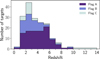 |
Fig. 4 Histogram of spectroscopic redshifts obtained from S/N > 5 emission lines. The separate histograms are for the medium-dispersion R ≈ 1000 gratings (flag A, darkest purple), additional galaxies with S/N > 5 emission lines detected with the low-dispersion R ≈ 30–300 prism (flag B, lighter purple histogram) and galaxies with more marginal redshifts (flag C, lightest histogram). |
5.3 Comments on individual targets
A few MSA shutters exhibited unusual spectral features, often due to more than one source in the shutter. We briefly discuss these below, along with objects which are likely to be stars where proper motion can be seen between the HST/WFC3 images and the JWST/NIRCam images taken ~13 years later.
5.3.1 ID 5293 – star
Proper motion can be identified between HST/WFC3 F775W imaging and JWST/NIRCam F277W imaging for this object. Furthermore the spectrum looks visually like a brown dwarf star. No proper motion was clearly seen when comparing different-epoch observations from HST alone – possibly due to the motion being comparable to the spatial resolution of HST/WFC3. However, with the better spatial resolution of NIRCam/SW, we detect a motion of ≈![$\[0^{\prime\prime}_\cdot05\]$](/articles/aa/full_html/2024/10/aa47094-23/aa47094-23-eq12.png) .
.
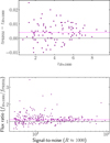 |
Fig. 5 Comparison of spectral measurements between the low-dispersion prism and medium-dispersion gratings. Upper: comparison of redshift as determined from Prism/Clear and R ≈ 1000 grating observations for targets with emission lines clearly detected in both modes. There is a systematic offset of Δz = 0.0039, with the prism yielding systematically higher redshifts. Lower: comparison of emission lines fluxes measured from prism and R ≈ 1000 grating. Measurements derived from the grating are systematically higher with a median value of fR≈1000/fprism = 1.105 and a standard deviation of 0.298. |
5.3.2 ID 7624 – two sources in shutter
Two sources can clearly be seen in the HST imaging (Figure 2), and the slit falls between the two sources. Object 7624 in Class 7.7 was the intended target (to the south of the slit), but a Lyman-break galaxy (a F435W b-band dropout) lies just to the north. We observe line detections consistent with [O III] 25007 and Hα at z = 2.665 (from the target object 7624) and also at z = 4.854 from the b-band drop-out.
5.3.3 ID 8896 – possible double source
This micro-shutter was originally targeted on a low redshift galaxy (Class 7.8). We detect at least three compelling emission lines, and one more marginal line. There are emission lines that are consistent with [O III] and Hα at z = 1.984, and this is reported in Table F.3. However, we note that there are two robust lines that are consistent with a z = 6.287 galaxy seen with [O III] and Hα. The imaging does not obviously reveal the presence of two objects (Figure 2), however there does not seem to be a plausible redshift solution that matches all of these lines simultaneously for a single object.
5.3.4 ID 9992 – possible double source
This object was targeted as a z > 8.5 candidate (Class 3). The Prism/CLEAR spectrum reveals a number of emission lines. The two most significant emission features are consistent with [O III] and Hα at z = 1.962. However, an emission line at 5.1 μm could be Hβ or [O III] λ5007 at z > 9, and this would be consistent with a tentative spectral break observed at 1.25 μm being a Lyman-α break. The NIRCam photometry reveals two components separated by only ![$\[0^{\prime\prime}_\cdot15\]$](/articles/aa/full_html/2024/10/aa47094-23/aa47094-23-eq13.png) (Figure 2). One of these is photometrically consistent with a drop-out galaxy at z ~ 10, while the other (over which the central shutter is better placed) is more consistent with lower redshift solutions. We do not consider our high redshift solution from the spectrum to be highly robust, and Table F.1 reports the low-redshift solution.
(Figure 2). One of these is photometrically consistent with a drop-out galaxy at z ~ 10, while the other (over which the central shutter is better placed) is more consistent with lower redshift solutions. We do not consider our high redshift solution from the spectrum to be highly robust, and Table F.1 reports the low-redshift solution.
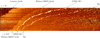 |
Fig. 6 Extracted 1D NIRSpec prism spectra of galaxies with good redshifts in the GOODS-South/HUDF field, ordered by redshift (with highest redshifts at the top). Each spectrum is plotted in flux units of fλλ1.5 (i.e. a galaxy with a spectral slope of β = −1.5 will have constant brightness with wavelength in this plot) and normalised by the mean intensity at 2.3 < λ < 4.45 μm. Wavelength increases to the right, from 0.6–5.3 μm. The Lyman-α break and Balmer/4000 Å break are clearly visible, as are the prominent emission lines Hα and the Hβ+[OIII] 4959,5007 complex (which is blended at low redshift but resolved at higher redshift). |
5.3.5 ID 10040 – multiple sources in shutter
Imaging clearly shows multiple sources with flux in the shutter. The spectrum has clear detections of emission lines consistent with [O III] and Hα at z = 3.14, which we report in Table F.3. There is also, however, continuum detected in the 2D spectrum, which appears to be spatially offset from the emission lines that we detect and which may arise from another source.
5.3.6 ID 10035328 – star
Proper motion can be identified between the HST/WFC3 images and the JWST/NIRCam images.
5.4 Quantifying the success of target selection
To measure the success of the class-based allocation, we looked at which targets from which classes actually ended up having the redshift expected (and desired line flux S /N in the case of Class 4).
In our highest-priority Class 1 (predicted redshifts z > 8.5 and AB < 29), we targeted six galaxies, five of which were robustly confirmed to be at high redshift: three at z > 11 have previously been reported in Curtis-Lake et al. (2023) (GSz12-0=2773 at z = 12.63, GSz11-0=10014220 at z = 11.58, GSz13-0=17400 at z = 13.20) and have strong Lyman-α breaks but no significant line emission. Galaxy 10058975 at z = 9.43 exhibits many strong emission lines (see Figure E.1), as does galaxy 8013 (which falls just below the targeted redshift cut at z = 8.47). One galaxy, ID 10014170, did not have obvious features in its spectrum and its redshift is ambiguous. Hence, we have a success rate of 83% in pre-selecting Priority Class 1 targets which are then spectroscopically confirmed to be at high redshift.
In Class 2 (candidates at z > 8.5 with AB < 29 which are more marginal), of the two targets one has a robust redshift of z = 9.68 (galaxy 6438), and the second target (galaxy 7300) has an inconclusive spectrum. Class 3 has three z > 8.5 candidates fainter than AB > 29, but even here we are successful in confirming the high redshift nature of some of these: of the three targets, ID 10014177 was previously reported in Curtis-Lake et al. (2023) as GSz10-0 at z = 10.38. Galaxy 9992 was discussed in Section 5.3.4; there is clearly a low-redshift interloper at z = 1.962, but inspection of the imaging reveals that there is a second galaxy, and the spectrum provides hints of other lines which may be consistent with a second source at z > 9. We regard this spectrum as inconclusive. The third galaxy (ID 6621) has no strong emission lines but may exhibit a spectral break consistent with a Lyman-α break at a tentative redshift of z = 9.6. Hence, for all 11 of the z > 8.5 candidates targeted, seven were clearly at high redshift (a fraction of 64%), and four had inconclusive redshifts (36%).
We now discuss the success of the selection in Class 4, where galaxies at 5.7 < z < 8.5 were targeted which were sufficiently bright (AB < 27.5 in the wavebands corresponding to the rest-UV) that high S /N emission lines are expected. Of the 20 sources in Class 4 which were targeted, 17 were confirmed to be at high redshift (including galaxy 16745 at z = 5.57, which fell just below the targeted redshift range). The emission line fluxes for Hα were typically brighter than 7.5 × 10⁻¹⁹ erg cm−2 s−1 (except for one object, ID 6384) as expected from our rest-UV preselection (Section 2). The uncertainty on the line flux from the prism is about 0.3 × 10⁻¹⁹ erg cm−2 s−1 as predicted, so we met our requirement of S/N > 25 in Hα for the sample in Class 4, enabling the physics of the ISM and the metal enrichment to be explored (Cameron et al. 2023; Curti et al. 2024). Our overall success rate in Class 4 is 85%, although we note that one of the three objects (out of 20) for which we did not obtain a good spectrum is ID 10035328, which is a likely star (see Section 5.3.6).
Fainter candidates than in Class 4 but in the same redshift interval 5.7 < z < 8.5 were placed in Class 6.1 if they were brighter than AB = 29 in HST/F160W (or the NIRCam filter around rest-frame 1500 Å), and in Class 6.2 if they were fainter than that. The success rate in Class 6.1 is very good, with eight of nine galaxies having redshifts in the targeted range. We note that object 8115 does not have emission lines but does a strong Lyman-α break and a weaker Balmer break at z = 7.3, and the JADES spectrum has been discussed in Looser et al. (2024) as a potential quiescent galaxy. The NIRSpec spectrum of ID 3334 at z = 6.71 has been presented in Witstok et al. (2023) and shows evidence of broad rest-frame UV absorption around 2175 Å. Object 3137 is a low-redshift interloper with z = 1.91, so our overall success rate in Class 6.1 is 89%. In the fainter Class 6.2, four of the seven objects have spectroscopic redshifts within the target range, with two galaxies also at redshifts slightly below this (object 8113 at z = 4.90 and object 17260 at z = 4.89). One spectrum (object 10014117) had no significant features from which a redshift could be determined. The NIRSpec spectrum of object 10013682 shows very strong Lyman-α emission at the systemic redshift of z = 7.28, as discussed in Saxena et al. (2023). Our success rate for Class 6.2 is 57%, rising to 86% if the two galaxies at z = 4.9 are included.
The success rate for Class 7 is recorded in Table 1 for the sub-classes 7.5–7.8, where there are significant numbers (>20) of galaxies targeted. Taking the metric for ‘success’ as being a measured spectroscopic redshift within Δz = 0.1 of the intended redshift range, we have success rates of 83% in the highest redshift slice (4.5 < z < 5.7, Class 7.5), around 80% for Classes 7.6 and 7.7, and 64% for the lowest redshift bin (1.5 < z < 2.5, Class 7.8). The interloper fractions were ≈3–4%, but these comprised galaxies only slightly outside the desried redshift bin (e.g. object 3892 has a redshift of z = 2.80 and was selected to be in Class 7.6 at 3.5 < z < 4.5). Those galaxies in Class 7 for which a reliable redshift could not be inferred amounted to <20% of those targeted, and these tended to be the sources which were less well centred within the shutters, resulting in large slit losses.
Overall our priority class pre-selection strategy seemed successful; for the more robust galaxies, 80% or more of the time the spectroscopic redshift fell in the anticipated range, and the line fluxes for Class 4 (which had been pre-selected on the basis of the rest-UV) were also as anticipated.
6 Conclusions
We have presented very deep spectroscopy obtained with JWST/NIRSpec in its multi-object MSA mode. In all, 253 targets were observed in this JADES Deep/HST spectroscopy covering the Hubble Ultra Deep Field, and the surrounding GOODS-South, with total integrations times of up to 28 hours for the low-dispersion prism (R ≈ 30–300), and up to 7 hours in the three medium dispersion gratings (R ≈ 1000) and one high dispersion grating (G395H, R ≈ 2700). We detected emission lines with S /N > 5 in 155 targets with the low-dispersion prism (see Figure 6), 103 of which also had emission lines detected at this significance in R ≈ 1000 gratings. The robust redshifts determined for these galaxies spanned a range from z = 0.66 to z = 13.2, with 18 lying at z > 6. A further 23 galaxies has more tentative redshifts. We are able to detect emission lines at S /N > 5 as faint as ≈ 10−19 erg cm−2 s−1 in our deepest prism spectra, and we have been able to confirm redshifts for some sources fainter than AB = 29. Our selection of targets preferentially places the rarer high redshift targets on the MSA at higher priority, with more numerous lower-redshift galaxies filling unused regions, so that we can probe a large redshift range from ‘cosmic noon’ (z ~ 2) to within the epoch of reionzation (z > 6) with reasonable numbers of galaxies in several redshift slices. We have demonstrated that our pre-selection of targets from HST and JWST imaging, based on broad-band magnitudes and photometric redshifts (including many Lyman break galaxy candidates) is highly effective, with ~80% of galaxies targeted having spectroscopic confirmation within the expected redshift bin. Hence our target selection and the quality and depth of the NIRSpec MSA spectroscopy means that our science goals for the JADES project can be met.
Data availability
Full versions of Tables F.1, F.2 and F.3 are available on https://arxiv.org/abs/2306.02467 and in electronic form at the CDS ftp to (130.79.128.5) or at https://cdsarc.cds.unistra.fr/viz-bin/cat/J/A+A/690/A288.
Acknowledgements
We sincerely thank Gabe Brammer for his work aligning HST imaging to the GAIA DR2 frame. In the absence of that work, this data release may well have amounted to 253 spectacularly deep spectra of empty sky. We thank the referee for helpful comments on this manuscript. The JADES Collaboration thanks the Instrument Development Teams and the instrument teams at the European Space Agency and the Space Telescope Science Institute for the support that made this program possible. We also thank our program coordinators at STScI for their help in planning complicated parallel observations. We thank all the members of the NIRSpec and NIRCam Instrument Science Teams for making these observations possible. AJB, AJC, AS, JC, GCJ, IW acknowledge funding from the “FirstGalaxies” Advanced Grant from the European Research Council (ERC) under the European Union’s Horizon 2020 research and innovation programme (Grant agreement No. 789056). ECL acknowledges support of an STFC Webb Fellowship (ST/W001438/1). The Cosmic Dawn Center (DAWN) is funded by the Danish National Research Foundation under grant no.140. SC acknowledges support by European Union’s HE ERC Starting Grant No. 101040227 – WINGS. RM, JW, FDE, TJL, WB, LS, JS acknowledges support by the Science and Technology Facilities Council (STFC) and by the ERC through Advanced Grant 695671 “QUENCH”. JW also acknowledges support from the Fondation MERAC. RS acknowledges support from a STFC Ernest Rutherford Fellowship (ST/S004831/1). SA, BRP acknowledges support from Grant PID2021-127718NB-I00 funded by the Spanish Ministry of Science and Innovation/State Agency of Research (MICIN/AEI/10.13039/501100011033). RB acknowledges support from an STFC Ernest Rutherford Fellowship [grant number ST/T003596/1]. This research is supported in part by the Australian Research Council Centre of Excellence for All Sky Astrophysics in 3 Dimensions (ASTRO 3D), through project number CE170100013. EE, BJD, MR, FS acknowledges the JWST/NIRCam contract to the University of Arizona NAS5-02015. DJE is supported as a Simons Investigator and by JWST/NIRCam contract to the University of Arizona, NAS5-02015. RH acknowledges funding provided by the Johns Hopkins University, Institute for Data Intensive Engineering and Science (IDIES). REH acknowledges acknowledges support from the National Science Foundation Graduate Research Fellowship Program under Grant No. DGE-1746060. MP acknowledges support from the research project PID2021-127718NB-I00 of the Spanish Ministry of Science and Innovation/State Agency of Research (MICIN/AEI/10.13039/501100011033), and the Programa Atracción de Talento de la Comunidad de Madrid via grant 2018-T2/TIC-11715. BER acknowledges support from the NIRCam Science Team contract to the University of Arizona, NAS5-02015. The research of CCW is supported by NOIRLab, which is managed by the Association of Universities for Research in Astronomy (AURA) under a cooperative agreement with the National Science Foundation. CW is supported by the National Science Foundation through the Graduate Research Fellowship Program funded by Grant Award No. DGE-1746060. This study made use of the Prospero high performance computing facility at Liverpool John Moores University. This work was performed using resources provided by the Cambridge Service for Data Driven Discovery (CSD3) operated by the University of Cambridge Research Computing Service (www.csd3.cam.ac.uk), provided by Dell EMC and Intel using Tier-2 funding from the Engineering and Physical Sciences Research Council (capital grant EP/T022159/1), and DiRAC funding from the Science and Technology Facilities Council (www.dirac.ac.uk). The authors acknowledge use of the lux supercomputer at UC Santa Cruz, funded by NSF MRI grant AST 1828315.
Appendix A Astrometry of HST-based targets
Astrometric offsets have previously been noted between previous reductions of HST imaging and other datasets registered to the GAIA DR2 astrometric frame (Dunlop et al. 2017; Franco et al. 2018; Whitaker et al. 2019). These studies have corrected the astrometry of CANDELS and 3DHST onto the Gaia DR2 frame (Gaia Collaboration 2016, 2018) with a bulk offset of 0.26 arcsec.
We used the Complete Hubble Archive for Galaxy Evolution (CHArGE) re-reduction of the HST imaging in GOODS-S, where all input frames have been carefully registered to the GAIA DR2 astrometric frame (Kokorev et al. 2022; Brammer 2023)5. In order to attain the astrometric accuracy required to ensure light is captured by an MSA shutter, we revisited the astrometry of the literature photometric candidates. For the large catalogues from 3DHST and UVUDF, and for the Lyman break surveys of Finkelstein et al. (2015) and Harikane et al. (2016), we matched the reported position of all brighter than F160W< 26 to the GAIA-DR2-registered catalogy=ue using ![$\[0^{\prime\prime}_\cdot5\]$](/articles/aa/full_html/2024/10/aa47094-23/aa47094-23-eq14.png) tolerance. Based on this, we identified that, in addition to the bulk offset previously identified, there was also a plate scale difference amounting to about 1 part in 5000. Across the full GOODSS field (10′ × 15′ in size) this amounts to systematic errors larger than the width of a micro-shutter, highlighting the need for correcting this effect.
tolerance. Based on this, we identified that, in addition to the bulk offset previously identified, there was also a plate scale difference amounting to about 1 part in 5000. Across the full GOODSS field (10′ × 15′ in size) this amounts to systematic errors larger than the width of a micro-shutter, highlighting the need for correcting this effect.
We fit a simple tangent-plane astrometric transformation allowing for a bulk offset, plate scale, and rotation to these offsets. We favoured the approach of fitting an astrometric transformation to the coordinates over re-measuring the centroids of objects in the CHArGE images because this new reduction had 100 mas drizzled pixels, and was not optimised for the selection of z ≳ 6 targets in the HUDF, where the HST data were deepest. Thus, many of of the targets that ended up in our highest priority classes were not clearly detected in these reductions.
Fitting this simple transformation to the Skelton et al. (2014) catalogue, we found that we reduced the residual RMS scatter on the positional offsets to 34 mas across the entire GOODS-South field. This corresponds to 17% of the illuminated NIRSpec slit width of ![$\[0^{\prime\prime}_\cdot2\]$](/articles/aa/full_html/2024/10/aa47094-23/aa47094-23-eq15.png) .
.
Given many of our highest priority targets were taken from Lyman-break catalogues, and did not necessarily appear in Skelton et al. (2014), we also constructed separate astrometric transformations for catalogues from Bouwens et al. (2015, 2021), Finkelstein et al. (2015) and Harikane et al. (2016). We found that very similar astrometric offsets were present in these catalogues, however the exact magnitude of each component of the correction varied slightly. The residuals on transformed coordinates were similarly ~30–50 mas after applying the relevant transformation.
We considered the corrections applied to Skelton et al. (2014) to be the most robust, since that catalogue had more entries than the Lyman-break catalogues. Thus, to obtain updated ‘GAIA DR2’ coordinates, we used the correction derived from Skelton et al. (2014) for all targets that had a counterpart in this catalogue.
In some cases, high-priority targets were not matched to a counterpart in the Skelton et al. (2014) catalogue, in which case we used a correction from the astrometric fit to one of the catalogues of Finkelstein et al. (2015), Harikane et al. (2016) or Bouwens et al. (2021) to obtain updated coordinates.
There were some cases where we placed high-priority targets that were not in one of the catalogues discussed above (e.g. Bouwens et al. 2011a and the z~10 candidate from McLure et al. 2013). In these case we remeasured the centroid using the latest HLF (Hubble Legacy Field) v2.0 reduction of the GOODS-South images, which we assessed as having astrometry in sufficiently good agreement with the GAIA DR2 frame.
Finally, we retained some targets in our catalogue for which we did not have a reliable conversion of the reported coordinates to the GAIA DR2 frame. However, these targets were flagged such that they could not appear any higher than Priority Class 9, and were only placed at the expense of extra sky shutters (Table 1).
Appendix B Caveats of early data release
At the time of target selection two weeks after the images were obtained, several issues present in the image reduction and analysis may have affected the prioritisation of the targets. The flat fields that were available at the time introduced spurious small-scale structure in the background at faint levels in some areas, leading to a large number of spurious detections close to the detection limit in those areas. Improvements to the flat fields since then will allow us to push to deeper limits in future targeting. In particular, Class 3 was designed to include fainter, less secure high redshift targets, but we retained those allocated from the HST pre-selection, and did not supplement with JWST-based sources fainter than AB = 29.5 mag. Improvements in the flat fielding, in the small and large scale background subtraction including wisps, and in the object deblending, especially near large bright sources, means that the current photometric measurements and source positions may differ from the very early estimates available at the time of target selection. In particular the Kron-based aperture measurements that were used for the flux cut in Class 7, which was designed to approach a total magnitude cut, were significantly impacted by these improvements.
Appendix C Slit Overlays of Targets
Figures C.1 – C.3, continued from Figure 2, showing the positions MSA shutter overlaid on observed targtes.
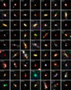 |
Fig. C.1 Overlay of target shutter positions onto the images for target IDs 7809–21598 sorted by NIRSpec ID number, starting at the top left. The illuminated shutter regions are outlined ( |
![$\[0^{\prime\prime}_\cdot46 \times 0^{\prime\prime}_\cdot20\]$](/articles/aa/full_html/2024/10/aa47094-23/aa47094-23-eq16.png)
![$\[1^{\prime\prime}_\cdot0\]$](/articles/aa/full_html/2024/10/aa47094-23/aa47094-23-eq17.png)
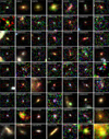 |
Fig. C.2 Overlay of target shutter positions onto the images for target IDs 21842–10011955 sorted by NIRSpec ID number, starting at the top left. The illuminated shutter regions are outlined ( |
![$\[0^{\prime\prime}_\cdot46 \times 0^{\prime\prime}_\cdot20\]$](/articles/aa/full_html/2024/10/aa47094-23/aa47094-23-eq18.png)
![$\[1^{\prime\prime}_\cdot0\]$](/articles/aa/full_html/2024/10/aa47094-23/aa47094-23-eq19.png)
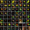 |
Fig. C.3 Overlay of target shutter positions onto the images for targets ID 10011974–10106979 sorted by NIRSpec ID number, starting at the top left. The illuminated shutter regions are outlined ( |
![$\[0^{\prime\prime}_\cdot46 \times 0^{\prime\prime}_\cdot20\]$](/articles/aa/full_html/2024/10/aa47094-23/aa47094-23-eq20.png)
![$\[1^{\prime\prime}_\cdot0\]$](/articles/aa/full_html/2024/10/aa47094-23/aa47094-23-eq21.png)
Appendix D Layout of Shutters in the HUDF/GOODS-South Field
Figures D.1 – D.3 continue from Figure 3, showing the remaining three quadrants of the MSA positioned on the field.
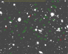 |
Fig. D.1 Quadrant 1 of the MSA, showing allocation of micro-shutters to targets. Those in green are covered by both the grating configurations and the low-dispersion prism. The red shutters are open only in the prism observations, as they would lead to overlapping spectra for our high priority targets in the grating configuration. Three micro-shutters are opened for each target, but the nodding by ±1 shutter means that spectra are obtained over the areas covered by five shutters (including background) which are displayed. The field displayed is the NIRCam F200W image. The yellow scale bar denotes 1 arcmin. North is up and East is to the left. Shutters with the prefix ‘B’ are empty sky background. |
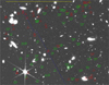 |
Fig. D.2 Quadrant 2 of the MSA, showing allocation of micro-shutters to targets. Those in green are covered by both the grating configurations and the low-dispersion prism. The red shutters are open only in the prism observations, as they would lead to overlapping spectra for our high priority targets in the grating configuration. Three micro-shutters are opened for each target, but the nodding by ±1 shutter means that spectra are obtained over the areas covered by five shutters (including background) which are displayed. North is up and East is to the left. The field displayed is the NIRCam F200W image, except for the area West of the blue line which had not yet been imaged by NIRCam and we show the HST F160W image. The yellow scale bar denotes 1 arcmin. Shutters with the prefix ‘B’ are empty sky background. |
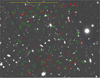 |
Fig. D.3 Quadrant 4 of the MSA, showing allocation of micro-shutters to targets. Those in green are covered by both the grating configurations and the low-dispersion prism. The red shutters are open only in the prism observations, as they would lead to overlapping spectra for our high priority targets in the grating configuration. Three micro-shutters are opened for each target, but the nodding by ±1 shutter means that spectra are obtained over the areas covered by five shutters (including background) which are displayed. North is up and East is to the left. The field displayed is the NIRCam F200W image, except for the area North-West of the blue line which had not yet been imaged by NIRCam and we show the HST F160W image. The yellow scale bar denotes 1 arcmin. Shutters with the prefix ‘B’ are empty sky background. |
Appendix E Example Spectra
Example spectra covering a range of redshifts are shown in Figures E.1–E.10. The low-dispersion prism spectrum is shown, along with the medium dispersion grating of emission prominent lines.
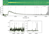 |
Fig. E.1 Low-dispersion prism spectra (1D and 2D) of 10058975 at z = 9.4327, with the medium dispersion grating of prominent lines shown below. Green shaded regions on the 1D spectra denote the 1σ errors. The wavelengths of common emission lines are denoted by vertical lines. |
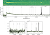 |
Fig. E.2 As for Figure E.1, but showing galaxy 021842 at z = 7.9806. |
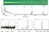 |
Fig. E.3 As for Figure E.1, but showing galaxy 018846 at z = 6.33. |
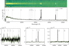 |
Fig. E.4 As for Figure E.1, but showing galaxy 022251 at z = 5.79. |
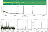 |
Fig. E.5 As for Figure E.1, but showing galaxy 018090 at z = 4.77. |
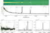 |
Fig. E.6 As for Figure E.1, but showing galaxy 007892 at z = 4.2287. |
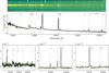 |
Fig. E.7 As for Figure E.1, but showing galaxy 018970 at z = 3.7245. Note the Balmer break just below [OII] 3727. |
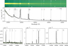 |
Fig. E.8 As for Figure E.1, but showing galaxy 003892 at z = 2.8072. Note the Balmer break just below [OII] 3727. |
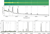 |
Fig. E.9 As for Figure E.1, but showing galaxy 003892 at z = 2.227. Note the Balmer break just below [OII] 3727. |
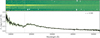 |
Fig. E.10 Prism spectra (1D and 2D) of 10036262, a galaxy which does not exhibit strong line emission but has a clear spectral break corresponding to a Balmer/4000 Å break at z = 3.566. |
Appendix F Tables of targets
We present tables of the priority classes and positions for each object observed (Table F.1), and the fluxes of lines detected at S/N > 5 in the medium dispersion grating spectra (Table F.2) and the low-dispersion prism spectra (Table F.3), along with the derived redshifts.
Table of targeted sources, ranked in priority order for placement on the MSA (highest priority at the top) – truncated table, full version on https://arxiv.org/abs/2306.02467 and at the CDS.
List of targets with one or more emission lines detected with S /N > 5 in the R ≈ 1000 grating data, and derived redshifts – truncated table, full version on https://arxiv.org/abs/2306.02467 and at the CDS.
List of targets with one or more emission lines detected at S/N > 5 in the Prism/Clear data – truncated table, full version on https://arxiv.org/abs/2306.02467 and at the CDS.
Targets not meeting the S/N > 5 emission line threshhold required to appear in Tables F.2 – F.3, but for which a secure redshift could be identified visually based on spectral breaks or low S /N emission features.
References
- Alonso-Herrero, A., Pérez-González, P. G., Alexander, D. M., et al. 2006, ApJ, 640, 167 [Google Scholar]
- Alves de Oliveira, C., Birkmann, S. M., Böker, T., et al. 2018, SPIE Conf. Ser., 10704, 107040Q [NASA ADS] [Google Scholar]
- Aravena, M., Decarli, R., Walter, F., et al. 2016, ApJ, 833, 68 [Google Scholar]
- Beckwith, S. V. W., Stiavelli, M., Koekemoer, A. M., et al. 2006, AJ, 132, 1729 [Google Scholar]
- Bonaventura, N., Jakobsen, P., Ferruit, P., Arribas, S., & Giardino, G. 2023, A&A, 672, A40 [NASA ADS] [CrossRef] [EDP Sciences] [Google Scholar]
- Bouwens, R. J., Illingworth, G. D., Blakeslee, J. P., & Franx, M. 2006, ApJ, 653, 53 [NASA ADS] [CrossRef] [Google Scholar]
- Bouwens, R. J., Illingworth, G. D., Oesch, P. A., et al. 2010, ApJ, 709, L133 [CrossRef] [Google Scholar]
- Bouwens, R. J., Illingworth, G. D., Labbe, I., et al. 2011a, Nature, 469, 504 [NASA ADS] [CrossRef] [Google Scholar]
- Bouwens, R. J., Illingworth, G. D., Oesch, P. A., et al. 2011b, ApJ, 737, 90 [NASA ADS] [CrossRef] [Google Scholar]
- Bouwens, R. J., Illingworth, G. D., Oesch, P. A., et al. 2015, ApJ, 803, 34 [Google Scholar]
- Bouwens, R. J., Oesch, P. A., Labbé, I., et al. 2016, ApJ, 830, 67 [Google Scholar]
- Bouwens, R. J., Oesch, P. A., Stefanon, M., et al. 2021, AJ, 162, 47 [NASA ADS] [CrossRef] [Google Scholar]
- Brammer, G. 2023, https://doi.org/10.5281/zenodo.8370018 [Google Scholar]
- Brammer, G. B., van Dokkum, P. G., & Coppi, P. 2008, ApJ, 686, 1503 [Google Scholar]
- Brammer, G. B., van Dokkum, P. G., Franx, M., et al. 2012, ApJS, 200, 13 [Google Scholar]
- Bunker, A. J., Stanway, E. R., Ellis, R. S., & McMahon, R. G. 2004, MNRAS, 355, 374 [NASA ADS] [CrossRef] [Google Scholar]
- Bunker, A. J., Wilkins, S., Ellis, R. S., et al. 2010, MNRAS, 409, 855 [Google Scholar]
- Bunker, A. J., NIRSPEC Instrument Science Team, & JADESs Collaboration 2020, in Uncovering Early Galaxy Evolution in the ALMA and JWST Era, 32, eds. E. da Cunha, J. Hodge, J. Afonso, L. Pentericci, & D. Sobral, 342 [Google Scholar]
- Bunker, A. J., Saxena, A., Cameron, A. J., et al. 2023, A&A, 677, A88 [NASA ADS] [CrossRef] [EDP Sciences] [Google Scholar]
- Cameron, A. J., Saxena, A., Bunker, A. J., et al. 2023, A&A, 677, A115 [NASA ADS] [CrossRef] [EDP Sciences] [Google Scholar]
- Carnall, A. C., McLure, R. J., Dunlop, J. S., & Davé, R. 2018, MNRAS, 480, 4379 [Google Scholar]
- Carnall, A. C., McLure, R. J., Dunlop, J. S., et al. 2019, MNRAS, 490, 417 [Google Scholar]
- Castelló-Mor, N., Carrera, F. J., Alonso-Herrero, A., et al. 2013, A&A, 556, A114 [NASA ADS] [CrossRef] [EDP Sciences] [Google Scholar]
- Chevallard, J., & Charlot, S. 2016, MNRAS, 462, 1415 [NASA ADS] [CrossRef] [Google Scholar]
- Coe, D., Benítez, N., Sánchez, S. F., et al. 2006, AJ, 132, 926 [Google Scholar]
- Curti, M., Maiolino, R., Curtis-Lake, E., et al. 2024, A&A, 684, A75 [NASA ADS] [CrossRef] [EDP Sciences] [Google Scholar]
- Curtis-Lake, E., Carniani, S., Cameron, A., et al. 2023, Nat. Astron., 7, 622 [NASA ADS] [CrossRef] [Google Scholar]
- Decarli, R., Walter, F., Aravena, M., et al. 2016, ApJ, 833, 70 [NASA ADS] [CrossRef] [Google Scholar]
- Del Moro, A., Alexander, D. M., Bauer, F. E., et al. 2016, MNRAS, 456, 2105 [Google Scholar]
- Dickinson, M., Giavalisco, M., & GOODS Team 2003, in The Mass of Galaxies at Low and High Redshift, eds. R. Bender, & A. Renzini, 324 [Google Scholar]
- Dunlop, J. S., McLure, R. J., Biggs, A. D., et al. 2017, MNRAS, 466, 861 [Google Scholar]
- Eisenstein, D. J., Willott, C., Alberts, S., et al. 2023, arXiv e-prints [arXiv:2306.02465] [Google Scholar]
- Ellis, R. S., McLure, R. J., Dunlop, J. S., et al. 2013, ApJ, 763, L7 [NASA ADS] [CrossRef] [Google Scholar]
- Ferruit, P., Jakobsen, P., Giardino, G., et al. 2022, A&A, 661, A81 [NASA ADS] [CrossRef] [EDP Sciences] [Google Scholar]
- Finkelstein, S. L., Ryan, Russell E., J., Papovich, C., et al. 2015, ApJ, 810, 71 [NASA ADS] [CrossRef] [Google Scholar]
- Franco, M., Elbaz, D., Béthermin, M., et al. 2018, A&A, 620, A152 [NASA ADS] [CrossRef] [EDP Sciences] [Google Scholar]
- Gaia Collaboration (Prusti, T., et al.) 2016, A&A, 595, A1 [NASA ADS] [CrossRef] [EDP Sciences] [Google Scholar]
- Gaia Collaboration (Brown, A. G. A., et al.) 2018, A&A, 616, A1 [NASA ADS] [CrossRef] [EDP Sciences] [Google Scholar]
- Gardner, J. P., Mather, J. C., Abbott, R., et al. 2023, PASP, 135, 068001 [NASA ADS] [CrossRef] [Google Scholar]
- Giardino, G., Birkmann, S., Robberto, M., et al. 2019, PASP, 131, 094503 [NASA ADS] [CrossRef] [Google Scholar]
- Giavalisco, M., Ferguson, H. C., Koekemoer, A. M., et al. 2004, ApJ, 600, L93 [NASA ADS] [CrossRef] [Google Scholar]
- Grogin, N. A., Kocevski, D. D., Faber, S. M., et al. 2011, ApJS, 197, 35 [NASA ADS] [CrossRef] [Google Scholar]
- Guo, Y., Ferguson, H. C., Giavalisco, M., et al. 2013, ApJS, 207, 24 [NASA ADS] [CrossRef] [Google Scholar]
- Harikane, Y., Ouchi, M., Ono, Y., et al. 2016, ApJ, 821, 123 [NASA ADS] [CrossRef] [Google Scholar]
- Hodge, J. A., Karim, A., Smail, I., et al. 2013, ApJ, 768, 91 [Google Scholar]
- Illingworth, G., Magee, D., Bouwens, R., et al. 2016, arXiv e-prints [arXiv:1606.00841] [Google Scholar]
- Inami, H., Bacon, R., Brinchmann, J., et al. 2017, A&A, 608, A2 [NASA ADS] [CrossRef] [EDP Sciences] [Google Scholar]
- Jakobsen, P., Ferruit, P., Alves de Oliveira, C., et al. 2022, A&A, 661, A80 [NASA ADS] [CrossRef] [EDP Sciences] [Google Scholar]
- Jones, G. C., Bunker, A. J., Saxena, A., et al. 2024, A&A, 683, A238 [NASA ADS] [CrossRef] [EDP Sciences] [Google Scholar]
- Kennicutt, Robert C., J. 1998, ARA&A, 36, 189 [Google Scholar]
- Koekemoer, A. M., Faber, S. M., Ferguson, H. C., et al. 2011, ApJS, 197, 36 [NASA ADS] [CrossRef] [Google Scholar]
- Kokorev, V., Brammer, G., Fujimoto, S., et al. 2022, ApJS, 263, 38 [NASA ADS] [CrossRef] [Google Scholar]
- Leja, J., Tacchella, S., & Conroy, C. 2019, ApJ, 880, L9 [NASA ADS] [CrossRef] [Google Scholar]
- Looser, T. J., D’Eugenio, F., Maiolino, R., et al. 2024, Nature, 629, 53 [Google Scholar]
- Lorenzoni, S., Bunker, A. J., Wilkins, S. M., et al. 2011, MNRAS, 414, 1455 [NASA ADS] [CrossRef] [Google Scholar]
- Lorenzoni, S., Bunker, A. J., Wilkins, S. M., et al. 2013, MNRAS, 429, 150 [NASA ADS] [CrossRef] [Google Scholar]
- Luo, B., Brandt, W. N., Xue, Y. Q., et al. 2011, ApJ, 740, 37 [NASA ADS] [CrossRef] [Google Scholar]
- Luo, B., Brandt, W. N., Xue, Y. Q., et al. 2017, ApJS, 228, 2 [Google Scholar]
- McLure, R. J., Dunlop, J. S., Bowler, R. A. A., et al. 2013, MNRAS, 432, 2696 [Google Scholar]
- Oesch, P. A., Bouwens, R. J., Illingworth, G. D., et al. 2010, ApJ, 709, L16 [Google Scholar]
- Oesch, P. A., Bouwens, R. J., Illingworth, G. D., et al. 2013, ApJ, 773, 75 [NASA ADS] [CrossRef] [Google Scholar]
- Oke, J. B., & Gunn, J. E. 1983, ApJ, 266, 713 [NASA ADS] [CrossRef] [Google Scholar]
- Planck Collaboration VI. 2020, A&A, 641, A6 [NASA ADS] [CrossRef] [EDP Sciences] [Google Scholar]
- Popesso, P., Dickinson, M., Nonino, M., et al. 2009, A&A, 494, 443 [NASA ADS] [CrossRef] [EDP Sciences] [Google Scholar]
- Rafelski, M., Teplitz, H. I., Gardner, J. P., et al. 2015, AJ, 150, 31 [Google Scholar]
- Rauscher, B. J., Arendt, R. G., Fixsen, D. J., et al. 2017, PASP, 129, 105003 [NASA ADS] [CrossRef] [Google Scholar]
- Rawle, T. D., Giardino, G., Franz, D. E., et al. 2022, Proc. SPIE, 12180, 121803R [NASA ADS] [Google Scholar]
- Rieke, M. 2020, in Uncovering Early Galaxy Evolution in the ALMA and JWST Era, 352, eds. E. da Cunha, J. Hodge, J. Afonso, L. Pentericci, & D. Sobral, 337 [Google Scholar]
- Rieke, M. J., Robertson, B., Tacchella, S., et al. 2023, ApJS, 269, 16 [NASA ADS] [CrossRef] [Google Scholar]
- Rujopakarn, W., Dunlop, J. S., Rieke, G. H., et al. 2016, ApJ, 833, 12 [NASA ADS] [CrossRef] [Google Scholar]
- Salpeter, E. E. 1955, ApJ, 121, 161 [Google Scholar]
- Sandles, L., D’Eugenio, F., Maiolino, R., et al. 2023, arXiv e-prints [arXiv:2306.03931] [Google Scholar]
- Sarajedini, V. L., Koo, D. C., Klesman, A. J., et al. 2011, ApJ, 731, 97 [NASA ADS] [CrossRef] [Google Scholar]
- Saxena, A., Robertson, B. E., Bunker, A. J., et al. 2023, A&A, 678, A68 [NASA ADS] [CrossRef] [EDP Sciences] [Google Scholar]
- Saxena, A., Bunker, A. J., Jones, G. C., et al. 2024, A&A, 684, A84 [NASA ADS] [CrossRef] [EDP Sciences] [Google Scholar]
- Schenker, M. A., Robertson, B. E., Ellis, R. S., et al. 2013, ApJ, 768, 196 [Google Scholar]
- Skelton, R. E., Whitaker, K. E., Momcheva, I. G., et al. 2014, ApJS, 214, 24 [Google Scholar]
- Stefanon, M., Labbé, I., Oesch, P. A., et al. 2021, ApJS, 257, 68 [NASA ADS] [CrossRef] [Google Scholar]
- Treister, E., Urry, C. M., Van Duyne, J., et al. 2006, ApJ, 640, 603 [NASA ADS] [CrossRef] [Google Scholar]
- Treister, E., Cardamone, C. N., Schawinski, K., et al. 2009a, ApJ, 706, 535 [NASA ADS] [CrossRef] [Google Scholar]
- Treister, E., Virani, S., Gawiser, E., et al. 2009b, ApJ, 693, 1713 [NASA ADS] [CrossRef] [Google Scholar]
- Whitaker, K. E., Ashas, M., Illingworth, G., et al. 2019, ApJS, 244, 16 [CrossRef] [Google Scholar]
- Wilkins, S. M., Bunker, A. J., Lorenzoni, S., & Caruana, J. 2011, MNRAS, 411, 23 [NASA ADS] [CrossRef] [Google Scholar]
- Witstok, J., Shivaei, I., Smit, R., et al. 2023, Nature, 621, 267 [CrossRef] [Google Scholar]
- Yamaguchi, Y., Kohno, K., Hatsukade, B., et al. 2019, ApJ, 878, 73 [Google Scholar]
- Yan, H., & Windhorst, R. A. 2004, ApJ, 612, L93 [NASA ADS] [CrossRef] [Google Scholar]
- Yan, H.-J., Windhorst, R. A., Hathi, N. P., et al. 2010, Res. Astron. Astrophys., 10, 867 [CrossRef] [Google Scholar]
- Young, M., Brandt, W. N., Xue, Y. Q., et al. 2012, ApJ, 748, 124 [NASA ADS] [CrossRef] [Google Scholar]
After the original APT file for PID 1210 had been submitted and scheduled by STScI, an electrical short appearing in a column of the MSA (Rawle et al. 2022) necessitated that the three MSA configurations be modified and substituted.
All Tables
Table of targeted sources, ranked in priority order for placement on the MSA (highest priority at the top) – truncated table, full version on https://arxiv.org/abs/2306.02467 and at the CDS.
List of targets with one or more emission lines detected with S /N > 5 in the R ≈ 1000 grating data, and derived redshifts – truncated table, full version on https://arxiv.org/abs/2306.02467 and at the CDS.
List of targets with one or more emission lines detected at S/N > 5 in the Prism/Clear data – truncated table, full version on https://arxiv.org/abs/2306.02467 and at the CDS.
Targets not meeting the S/N > 5 emission line threshhold required to appear in Tables F.2 – F.3, but for which a secure redshift could be identified visually based on spectral breaks or low S /N emission features.
All Figures
|
Fig. 1 Field layout of the NIRSpec Deep-HST observations presented in this paper. The green rectange is the region covered by the original HST/ACS Hubble Ultra Deep Field. The red rectangle is the smaller area covered in the Ultra Deep HST/WFC 3 imaging. The background image is the NIRCam F200W from JADES, except for the region to the right of the blue line which has not yet been observed by NIRCam; we show in this region the HST/WFC 3 from GOODS-South/CANDELS in blue. The short red lines denote the five-shutter ( |
| In the text | |
|
Fig. 2 Overlay of target shutter positions onto the images, with the illuminated shutter regions outlined ( |
| In the text | |
|
Fig. 3 One of the four MSA quadrants (Q3), showing allocation of micro-shutters to targets. The other quadrants are shown in Appendix D. Those shutters in green are covered by both the grating configurations and the low-dispersion prism. The red shutters are open only in the prism observations, as they would lead to overlapping spectra for our high priority targets in the grating configuration. Three micro-shutters are opened for each target, but the nodding by ±1 shutter means that spectra are obtained over the areas covered by five shutters (including background) which are displayed. The field displayed is the NIRCam F200W image, and is 1.8 arcmin on a side. North is up and East is to the left. Shutters with the prefix ‘B’ are empty sky background. |
| In the text | |
|
Fig. 4 Histogram of spectroscopic redshifts obtained from S/N > 5 emission lines. The separate histograms are for the medium-dispersion R ≈ 1000 gratings (flag A, darkest purple), additional galaxies with S/N > 5 emission lines detected with the low-dispersion R ≈ 30–300 prism (flag B, lighter purple histogram) and galaxies with more marginal redshifts (flag C, lightest histogram). |
| In the text | |
|
Fig. 5 Comparison of spectral measurements between the low-dispersion prism and medium-dispersion gratings. Upper: comparison of redshift as determined from Prism/Clear and R ≈ 1000 grating observations for targets with emission lines clearly detected in both modes. There is a systematic offset of Δz = 0.0039, with the prism yielding systematically higher redshifts. Lower: comparison of emission lines fluxes measured from prism and R ≈ 1000 grating. Measurements derived from the grating are systematically higher with a median value of fR≈1000/fprism = 1.105 and a standard deviation of 0.298. |
| In the text | |
|
Fig. 6 Extracted 1D NIRSpec prism spectra of galaxies with good redshifts in the GOODS-South/HUDF field, ordered by redshift (with highest redshifts at the top). Each spectrum is plotted in flux units of fλλ1.5 (i.e. a galaxy with a spectral slope of β = −1.5 will have constant brightness with wavelength in this plot) and normalised by the mean intensity at 2.3 < λ < 4.45 μm. Wavelength increases to the right, from 0.6–5.3 μm. The Lyman-α break and Balmer/4000 Å break are clearly visible, as are the prominent emission lines Hα and the Hβ+[OIII] 4959,5007 complex (which is blended at low redshift but resolved at higher redshift). |
| In the text | |
|
Fig. C.1 Overlay of target shutter positions onto the images for target IDs 7809–21598 sorted by NIRSpec ID number, starting at the top left. The illuminated shutter regions are outlined ( |
| In the text | |
|
Fig. C.2 Overlay of target shutter positions onto the images for target IDs 21842–10011955 sorted by NIRSpec ID number, starting at the top left. The illuminated shutter regions are outlined ( |
| In the text | |
|
Fig. C.3 Overlay of target shutter positions onto the images for targets ID 10011974–10106979 sorted by NIRSpec ID number, starting at the top left. The illuminated shutter regions are outlined ( |
| In the text | |
|
Fig. D.1 Quadrant 1 of the MSA, showing allocation of micro-shutters to targets. Those in green are covered by both the grating configurations and the low-dispersion prism. The red shutters are open only in the prism observations, as they would lead to overlapping spectra for our high priority targets in the grating configuration. Three micro-shutters are opened for each target, but the nodding by ±1 shutter means that spectra are obtained over the areas covered by five shutters (including background) which are displayed. The field displayed is the NIRCam F200W image. The yellow scale bar denotes 1 arcmin. North is up and East is to the left. Shutters with the prefix ‘B’ are empty sky background. |
| In the text | |
|
Fig. D.2 Quadrant 2 of the MSA, showing allocation of micro-shutters to targets. Those in green are covered by both the grating configurations and the low-dispersion prism. The red shutters are open only in the prism observations, as they would lead to overlapping spectra for our high priority targets in the grating configuration. Three micro-shutters are opened for each target, but the nodding by ±1 shutter means that spectra are obtained over the areas covered by five shutters (including background) which are displayed. North is up and East is to the left. The field displayed is the NIRCam F200W image, except for the area West of the blue line which had not yet been imaged by NIRCam and we show the HST F160W image. The yellow scale bar denotes 1 arcmin. Shutters with the prefix ‘B’ are empty sky background. |
| In the text | |
|
Fig. D.3 Quadrant 4 of the MSA, showing allocation of micro-shutters to targets. Those in green are covered by both the grating configurations and the low-dispersion prism. The red shutters are open only in the prism observations, as they would lead to overlapping spectra for our high priority targets in the grating configuration. Three micro-shutters are opened for each target, but the nodding by ±1 shutter means that spectra are obtained over the areas covered by five shutters (including background) which are displayed. North is up and East is to the left. The field displayed is the NIRCam F200W image, except for the area North-West of the blue line which had not yet been imaged by NIRCam and we show the HST F160W image. The yellow scale bar denotes 1 arcmin. Shutters with the prefix ‘B’ are empty sky background. |
| In the text | |
|
Fig. E.1 Low-dispersion prism spectra (1D and 2D) of 10058975 at z = 9.4327, with the medium dispersion grating of prominent lines shown below. Green shaded regions on the 1D spectra denote the 1σ errors. The wavelengths of common emission lines are denoted by vertical lines. |
| In the text | |
|
Fig. E.2 As for Figure E.1, but showing galaxy 021842 at z = 7.9806. |
| In the text | |
|
Fig. E.3 As for Figure E.1, but showing galaxy 018846 at z = 6.33. |
| In the text | |
|
Fig. E.4 As for Figure E.1, but showing galaxy 022251 at z = 5.79. |
| In the text | |
|
Fig. E.5 As for Figure E.1, but showing galaxy 018090 at z = 4.77. |
| In the text | |
|
Fig. E.6 As for Figure E.1, but showing galaxy 007892 at z = 4.2287. |
| In the text | |
|
Fig. E.7 As for Figure E.1, but showing galaxy 018970 at z = 3.7245. Note the Balmer break just below [OII] 3727. |
| In the text | |
|
Fig. E.8 As for Figure E.1, but showing galaxy 003892 at z = 2.8072. Note the Balmer break just below [OII] 3727. |
| In the text | |
|
Fig. E.9 As for Figure E.1, but showing galaxy 003892 at z = 2.227. Note the Balmer break just below [OII] 3727. |
| In the text | |
|
Fig. E.10 Prism spectra (1D and 2D) of 10036262, a galaxy which does not exhibit strong line emission but has a clear spectral break corresponding to a Balmer/4000 Å break at z = 3.566. |
| In the text | |
Current usage metrics show cumulative count of Article Views (full-text article views including HTML views, PDF and ePub downloads, according to the available data) and Abstracts Views on Vision4Press platform.
Data correspond to usage on the plateform after 2015. The current usage metrics is available 48-96 hours after online publication and is updated daily on week days.
Initial download of the metrics may take a while.