| Issue |
A&A
Volume 684, April 2024
|
|
|---|---|---|
| Article Number | A87 | |
| Number of page(s) | 17 | |
| Section | Extragalactic astronomy | |
| DOI | https://doi.org/10.1051/0004-6361/202347755 | |
| Published online | 05 April 2024 | |
Ionised gas kinematics and dynamical masses of z ≳ 6 galaxies from JADES/NIRSpec high-resolution spectroscopy
1
Max-Planck-Institut für Astronomie, Königstuhl 17, 69117 Heidelberg, Germany
e-mail: This email address is being protected from spambots. You need JavaScript enabled to view it.
2
Scuola Normale Superiore, Piazza dei Cavalieri 7, 56126 Pisa, Italy
3
Department of Astronomy and Astrophysics University of California, Santa Cruz, 1156 High Street, Santa Cruz, CA 96054, USA
4
Kavli Institute for Particle Astrophysics and Cosmology and Department of Physics, Stanford University, Stanford, CA 94305, USA
5
Sorbonne Université, CNRS, UMR 7095, Institut d’Astrophysique de Paris, 98 bis bd Arago, 75014 Paris, France
6
Centre for Astrophysics Research, Department of Physics, Astronomy and Mathematics, University of Hertfordshire, Hatfield AL10 9AB, UK
7
Centro de Astrobiología (CAB), CSIC–INTA, Cra. de Ajalvir Km. 4, 28850 Torrejón de Ardoz, Madrid, Spain
8
Kavli Institute for Cosmology, University of Cambridge, Madingley Road, Cambridge CB3 0HA, UK
9
Cavendish Laboratory – Astrophysics Group, University of Cambridge, 19 JJ Thomson Avenue, Cambridge CB3 0HE, UK
10
School of Physics, University of Melbourne, Parkville, 3010 VIC, Australia
11
ARC Centre of Excellence for All Sky Astrophysics in 3 Dimensions (ASTRO 3D), Australia
12
Department of Physics, University of Oxford, Denys Wilkinson Building, Keble Road, Oxford OX1 3RH, UK
13
European Southern Observatory, Karl-Schwarzschild-Strasse 2, 85748 Garching, Germany
14
Center for Astrophysics | Harvard & Smithsonian, 60 Garden St., Cambridge, MA 02138, USA
15
Leiden Observatory, Leiden University, PO Box 9513 2300 AA Leiden, The Netherlands
16
Steward Observatory, University of Arizona, 933 N. Cherry Avenue, Tucson, AZ 85721, USA
17
Department of Physics and Astronomy, The Johns Hopkins University, 3400 N. Charles St., Baltimore, MD 21218, USA
18
Department of Physics and Astronomy, University College London, Gower Street, London WC1E 6BT, UK
19
Department of Astronomy, University of Wisconsin-Madison, 475 N. Charter St., Madison, WI 53706, USA
20
Department for Astrophysical and Planetary Science, University of Colorado, Boulder, CO 80309, USA
21
European Space Agency (ESA), European Space Astronomy Centre (ESAC), Camino Bajo del Castillo s/n, 28692 Villafranca del Castillo, Madrid, Spain
22
NSF’s National Optical-Infrared Astronomy Research Laboratory, 950 North Cherry Avenue, Tucson, AZ 85719, USA
23
NRC Herzberg, 5071 West Saanich Rd, Victoria, BC V9E 2E7, Canada
Received:
18
August
2023
Accepted:
18
December
2023
Abstract
We explore the kinematic gas properties of six 5.5 < z < 7.4 galaxies in the JWST Advanced Deep Extragalactic Survey (JADES), using high-resolution JWST/NIRSpec multi-object spectroscopy of the rest-frame optical emission lines [OIII] and Hα. The objects are small and of low stellar mass (∼1 kpc; M* ∼ 107 − 9 M⊙), less massive than any galaxy studied kinematically at z > 1 thus far. The cold gas masses implied by the observed star formation rates are about ten times higher than the stellar masses. We find that their ionised gas is spatially resolved by JWST, with evidence for broadened lines and spatial velocity gradients. Using a simple thin-disc model, we fit these data with a novel forward-modelling software that accounts for the complex geometry, point spread function, and pixellation of the NIRSpec instrument. We find the sample to include both rotation- and dispersion-dominated structures, as we detect velocity gradients of v(re)∼100 − 150 km s−1, and we find velocity dispersions of σ0 ∼ 30 − 70 km s−1 that are comparable to those at cosmic noon. The dynamical masses implied by these models (Mdyn ∼ 109 − 10 M⊙) are higher than the stellar masses by up to a factor 40, and they are higher than the total baryonic mass (gas + stars) by a factor of ∼3. Qualitatively, this result is robust even if the observed velocity gradients reflect ongoing mergers rather than rotating discs. Unless the observed emission line kinematics is dominated by outflows, this implies that the centres of these galaxies are dominated by dark matter or that star formation is three times less efficient, leading to higher inferred gas masses.
Key words: galaxies: evolution / galaxies: high-redshift / galaxies: kinematics and dynamics / galaxies: structure
© The Authors 2024
 Open Access article, published by EDP Sciences, under the terms of the Creative Commons Attribution License (https://creativecommons.org/licenses/by/4.0), which permits unrestricted use, distribution, and reproduction in any medium, provided the original work is properly cited.
This article is published in open access under the Subscribe to Open model.
Open Access funding provided by Max Planck Society.
1. Introduction
In the nearby Universe, galaxies show a variety of dynamical structures and structural components that reflect their mass-assembly histories (e.g., Cappellari 2016; van de Sande et al. 2018; Falcón-Barroso et al. 2019). However, the details of the formation and evolution of these structures, which nominally are rotationally supported discs and spheroidal bulges supported primarily by dispersion, are still unclear. The physical conditions in the early Universe, the secular evolution of galaxies, and mergers with other systems are all likely to play important roles. One outstanding question in particular is when and how early galaxies settled into dynamically cold discs.
Although this question is ideally answered by measuring spatially resolved stellar kinematics across cosmic time, such measurements have only been possible up to z ∼ 1 (e.g., van Houdt et al. 2021), except for a few strongly lensed massive galaxies at z ∼ 2 (Newman et al. 2018). Instead, the ionised gas of the interstellar medium (ISM) provides critical insight into the dynamical properties of (star-forming) galaxies across a much wider redshift range (for a review, see Förster Schreiber & Wuyts 2020). Many studies have focused on inferring galaxy dynamical properties from rest-frame optical emission lines to map the evolution in the velocity dispersion (σ) and the ratio of the rotation velocity and dispersion (v/σ), which measures the degree of rotational support of the system.
Measurements of the ionised gas kinematics from multiple large spectroscopic surveys of star-forming galaxies at z ∼ 1 − 4 have demonstrated that the velocity dispersion of star-forming galaxies increases with redshift, while the rotational support decreases to v/σ ∼ 1 by z ∼ 3 (e.g., Wisnioski et al. 2015, 2019; Stott et al. 2016; Simons et al. 2017; Turner et al. 2017; Price et al. 2020). In addition, imaging studies have shown that galaxy morphologies are less disc-like and more clumpy at rest-frame UV wavelengths at higher redshifts (e.g., van der Wel et al. 2014; Guo et al. 2015; Zhang et al. 2019; Sattari et al. 2023). Theoretical models and simulations have suggested that gravitational instabilities, the accretion of gas and smaller systems from the cosmic web, and stellar feedback may cause the increased turbulence at higher redshifts (e.g., Dekel et al. 2009b; Genel et al. 2012; Ceverino et al. 2012; Krumholz et al. 2018).
However, using submillimeter observations from the Atacama Large Millimeter Array (ALMA), several studies have found dynamically cold discs at z ∼ 2 − 6 (e.g., Neeleman et al. 2020; Jones et al. 2021; Lelli et al. 2021; Rizzo et al. 2021; Parlanti et al. 2023; Pope et al. 2023), even finding v/σ ∼ 20 at z = 4.5 (Fraternali et al. 2021). These observations raise the question of how such systems formed and settled so rapidly (within ∼1 Gyr), and how these observations can be reconciled with the aforementioned studies at cosmic noon. However, the ALMA observations infer the galaxy kinematics from far-infrared and millimetre transitions (CO, [CII]), which trace colder gas than the rest-frame optical lines, likely explaining part of the discrepancy (Übler et al. 2019; Rizzo et al. 2023). Additionally, selection effects likely play an important role, as many of the ALMA observations primarily probe the most massive galaxies at z > 4.
To understand the evolution of more typical (∼M*) galaxies requires spatially resolved spectroscopy of faint galaxies at high redshifts. In this regime, ground-based telescopes are unable to observe rest-frame optical emission lines, whereas submillimeter (submm) facilities are in principle able to observe such systems, but at extremely high cost. The launch of the James Webb Space Telescope (JWST) has enabled spectroscopy with very high sensitivity and high spatial resolution (Gardner et al. 2023; Rigby et al. 2023). Using the slitless spectroscopy mode of JWST/NIRCam (Rieke et al. 2023a), Nelson et al. (in prep.) reveal the ionised gas kinematics in a massive galaxy at z ∼ 5. However, only the NIRSpec instrument provides the spectral resolution needed to resolve galaxy kinematics for low-mass systems (σ ∼ 50 km s−1 for a uniformly-illuminated slit; Jakobsen et al. 2022). JWST/NIRSpec additionally provides a multi-object spectroscopic (MOS) mode (Ferruit et al. 2022), allowing for the simultaneous observation of ∼200 objects, making observations of high-redshift targets highly efficient. The slit-based observations with the microshutter array (MSA), however, sacrifice one spatial dimension with respect to integral field spectroscopy (IFS; Böker et al. 2022, see also Price et al. 2016). Therefore, extra care is required to extract spatial and dynamical information from NIRSpec MSA data.
In this paper, we present the dynamical properties of six high-redshift galaxies (z > 5.5) in the JWST Advanced Deep Extragalactic Survey (JADES; Eisenstein et al. 2023). These objects are spatially extended in deep NIRCam imaging and were followed up with the high-resolution NIRSpec MOS mode, providing spatially resolved spectroscopy of their rest-frame optical emission lines. The data are presented in Sect. 2. To model the galaxy kinematics, we propagated analytical models through a simulated NIRSpec instrument, and used Markov chain Monte Carlo (MCMC) sampling to fit the data (Sect. 3), using NIRCam imaging as a prior on the morphology. We present the results of our modelling in Sect. 4, demonstrating a diverse range of kinematic structures in a previously unexplored population of galaxies. We discuss the possibility that some systems may be late-stage mergers in Sect. 5, and examine the large discrepancy between the derived dynamical and stellar masses. We summarise our findings in Sect. 6.
2. Data
2.1. NIRSpec spectroscopy
We used NIRSpec MOS observations in the Great Observatories Origins Deep Survey South (GOODS-S) field taken as part of the JADES deep and medium programmes (ID numbers 1210 and 1286, PI N. Lützgendorf; Bunker et al. 2023; Eisenstein et al. 2023). The targets were selected from a combination of JWST/NIRCam and Hubble Space Telescope (HST) imaging and were followed up with JWST/NIRSpec using the low-resolution prism (R ∼ 100), the three medium-resolution gratings (R ∼ 1000), and the reddest high-resolution grating (G395H; R ∼ 2700 for a uniformly illuminated slit). Here, we focus primarily on the high-resolution spectroscopy, although we also used the prism data to estimate stellar masses and star formation rates (SFRs). The spectra in our sample were obtained using a three-point nodding pattern, and they vary in depth, ranging from 2.2 h to 7.0 h of total integration time for the G395H grating (summarised in Table 1). The total exposure times for the prism range from 2.2 h to 28 h.
Coordinates and G395H exposure times of the selected sample.
The NIRSpec data were reduced using the NIRSpec guaranteed time observations (GTO) collaboration pipeline (Carniani et al. in prep), which is also described in Curtis-Lake et al. (2023) and Bunker et al. (2023). Crucially, in contrast with other studies using NIRSpec data so far, our analysis largely does not rely on the final rectified, combined, and extracted 2D and 1D spectra generated by the pipeline. Instead, we perform our dynamical modelling to intermediate data products: We use 2D cutouts of the detector from individual exposures that were background subtracted and flat fielded. In this way, we mitigate correlated noise and artificial broadening that is otherwise introduced by the rectification and combination algorithm of the reduction pipeline. We also note that these intermediate data products do not correct for any slit losses due to the spatial extent of the sources because these effects are already fully accounted for in our modelling (Sect. 3).
Nevertheless, the 2D rectified high-resolution spectra and their 1D extractions were used for the initial visual inspection and selection of the sample. We also used the 1D extracted prism data for spectral energy distribution (SED) modelling in Sect. 4 to estimate stellar masses and SFRs.
2.2. NIRCam imaging
Even though some objects were initially selected based on HST imaging, JWST/NIRCam imaging is available for all targets in our sample from a combination of Cycle 1 programmes. The majority of our targets fall within the JADES footprint in GOODS-S (Rieke et al. 2023b), and are therefore imaged in nine different NIRCam filters. One of the selected targets (JADES-NS-10016374) is located outside of the JADES footprint, but falls within the footprint of the First Reionization Epoch Spectroscopically Complete Observations (FRESCO) survey (programme 1895, PI P. Oesch; Oesch et al. 2023). Although FRESCO is primarily a grism survey, the survey also obtained imaging with three different NIRCam filters (F182M, F210M, and F444W), although at significantly reduced exposure times compared with JADES imaging.
All images were reduced as described in Rieke et al. (2023b). We used the JWST calibration pipeline v1.9.6 with the CRDS pipeline mapping (pmap) context 1084. We ran stages 1 and 2 of the pipeline with the default parameters, but provided our own sky-flat for the flat-fielding. Following stage 2, we performed a custom subtraction of the 1/f noise, scattered-light effects (“wisps”), and the large-scale background. We performed an astrometric alignment using a custom version of JWST TweakReg, aligning our images to the HST F814W and F160W mosaics in the GOODS-S field with astrometry tied to the Gaia Early Data Release 3 (EDR3; G. Brammer, priv. comm.). We achieved an overall good alignment with relative offsets between bands of less than 0.1 short-wavelength pixel (< 3 mas). We then ran stage 3 of the JWST pipeline, combining all exposures of a given filter and a given visit.
For our analysis, we selected the NIRCam filter that most closely represents the emission line morphology of the target. Given the high equivalent widths of the emission lines in our sample, we used the medium band covering the emission line where available (four out of six objects). For the remaining two objects, we instead used broad-band filters. We use the available low-resolution prism spectra to quantify the flux originating from emission lines versus the stellar continuum in Appendix B. For the four objects with medium-band images, we hence estimate that ∼70 − 75% of the NIRCam flux is due to emission lines, and therefore provide a good map of the ionised gas. For the two objects with broad-band images, the stellar continuum dominates (emission line fluxes contribute ∼35%), and we discuss how this may affect the inferred kinematic parameters in Sects. 4 and 5.2.
2.3. Sample selection
We visually inspected all (358) JADES targets in GOODS-S for which high-resolution NIRSpec spectroscopy is available thus far. We selected objects that are at high redshift (z > 5.5, i.e. when the Universe was less than 1 Gyr old), are spatially extended in the NIRCam imaging (re ≳ 0.1″), and have bright emission lines, that is, an integrated signal-to-noise ratio (S/N) ≳ 20. Additionally, we required that the 1D spectrum showed no obvious evidence for a broad-line component, which would be indicative of large-scale outflows (i.e., the sample discussed in Carniani et al. 2023). The resulting sample consists of six objects that span the redshift range z = 5.5 − 7.4. We observe Hα in two of these objects, and [OIII] in the remaining four. For the two highest-redshift targets, Hα is outside the wavelength coverage of NIRSpec (z > 7). For two z ∼ 6 objects, we do not observe Hα because the traces of the high-resolution spectra are long and therefore fall partially off the detector.
The 2D combined and rectified images of the emission lines are presented in Fig. 1 together with cutouts from the NIRCam imaging, where we selected the NIRCam filter closest to the emission line as described in the previous section. The positions of the microshutters are shown in orange.
 |
Fig. 1. Sample of six spatially resolved high-redshift objects in JADES. The left panels show cutouts of the emission lines in the 2D rectified and combined spectra obtained with the high-resolution G395H grating. The negatives in the cutouts are the result of the background-subtraction method. The right panels show NIRCam image cutouts for each object (JADES and FRESCO) for the band that most closely resembles the emission line morphology (Sect. 2.2). The three-shutter slits and three-point nodding pattern we used result in an effective area of five shutters: The shutter encompassing the source is shown in orange, and the shutters used for background subtraction are shown in purple. |
We note that given the complex selection function of JADES (Bunker et al. 2023) and our additional imposed selection criteria during the visual inspection, the selected sample is far from complete in (stellar) mass, magnitude, or SFR. However, our aim is to demonstrate the ability of NIRSpec/MOS of measuring galaxy kinematics in an entirely new regime: Fig. 2 shows that the targets in our sample are not only at a higher redshift than has been attainable so far with ground-based near-infrared spectrographs, but they are also significantly smaller and less massive. We defer a comprehensive analysis of the galaxy kinematics as a function of redshift and mass to a future paper, as this will require the complete JADES and NIRSpec WIDE datasets (Eisenstein et al. 2023; Maseda et al., in prep.) as well as a thorough understanding of the selection functions of the different survey tiers.
 |
Fig. 2. Sample distribution in the parameter space of the stellar mass, SFR, and emission line half-light radius, colour-coded by redshift. We compare this with a selection of ground-based near-infrared spectroscopic surveys that used the Hα and [OIII] lines to measure galaxy kinematics at z ∼ 1 − 4 (Turner et al. 2017; Förster Schreiber et al. 2018; Wisnioski et al. 2019; Price et al. 2020). We used UV+IR SFRs from Whitaker et al. (2014) where available for the Turner et al. (2017) sample. We note that all objects at z > 1 from KMOS3D are shown in this figure, but not all objects were used in the kinematic studies because the S/N was low or the objects were too small. The sample selected from JADES (hexagons) probes a very different regime: JADES targets are at higher redshift and lower stellar mass than ground-based facilities have probed thus far. |
3. Dynamical modelling
We used a Bayesian forward-modelling approach to estimate the dynamical properties of the galaxies from 2D emission spectra, observed through the NIRSpec MSA apertures. First, we constructed parametric model cubes for the flux distribution (I(x, λ)) based on analytical surface brightness and velocity profiles. Second, we modelled the complexities of the NIRSpec instrument that are imprinted on the data when mapping the kinematic models onto a mock NIRSpec detector. Third, we used an MCMC sampling method to fit the models to the spectra, adopting Sérsic profile fits to NIRCam imaging as a prior. We defer a detailed description of this forward-modelling and fitting software (msafit) to a future paper, in which we will also demonstrate convergence tests and comparison with calibration data. In this section, we only provide a summary overview of the models and software, which we release publicly together with this paper1.
3.1. Thin-disc models
Although the spatial and spectral resolution of JWST/NIRSpec are high, the small systems in our sample are close to the resolution limit. This suggests that we should limit ourselves to a relatively simple geometric and dynamical model: a thin rotating disc. Although geometrically thin, we allowed for the disc to be kinematically warm by adding a velocity dispersion profile. We discuss the possible limitations of our model choice in Sect. 5.
We modelled the spatial flux distribution of the emission line as a Sérsic profile (Sérsic 1968), which is described by four parameters: the total flux F, the half-light radius re (major axis), the projected minor-to-major axis ratio q, and the Sérsic index n. As we assumed a thin-disc model, the projected axis ratio is directly related to the inclination angle (i) of the system. In addition, three important position-dependent parameters enter the model: the position angle (PA) with respect to the MSA slitlet as measured from the positive x-axis (i.e. PA = 90 deg represents perfect alignment with the slit), and the centroid position (dx, dy) of the object within the shutter.
For the velocity field, we used the common empirical description of an arctangent rotation curve (Courteau 1997),
 (1)
(1)
where va is the asymptotic or maximum velocity with respect to the systemic velocity of the galaxy, and rt is the turnover radius. We parametrised the systemic velocity as the mean wavelength of the emission line λ0. To allow for a kinematically warm disc, we additionally assumed a constant velocity dispersion profile σ(r)≡σ0 across the disc.
Combined, this amounts to a 11-parameter model (λ0, F, dx, dy, re, n, q, PA, rt, va, and σ0). We convolved the flux profile and velocity profiles to form a model flux cube I(x, y, λ), where x and y are the coordinates in the MSA plane and sampled in user-specified intervals. To construct these cubes, we ensured that the spatial and wavelength dimensions were sampled at minimum at Nyquist frequency for the point spread function (PSF) at the wavelength considered or the NIRSpec pixel size (0.1″), whichever was smaller. However, this sampling would be too sparse to evaluate the steep Sérsic profiles at small radii. In order to accurately integrate Sérsic profiles, we therefore first oversampled the spatial grid dynamically, such that the innermost region (< 0.2 re) was oversampled by a factor of 500 and the outer regions (> re) by a factor of 10, and then integrated the profile onto the coarser grid.
3.2. Forward-modelling the NIRSpec MSA
Although forward-modelling software for slit-based multi-object spectroscopy has been developed before (Price et al. 2016), there are several unique challenges to modelling NIRSpec MOS data: (i) The diffraction-limited PSF of JWST, which enables high spatial resolution, but is highly complex in shape. (ii) The complex geometry of the NIRSpec MSA, comprising ∼2 × 10⁵ microshutters that are separated by shutter walls, imprints additional diffraction patterns (plus-shaped due to the slit aperture) as well as shadows on the detector (“bar shadows”). Finally, (iii) the relatively large pixels (∼0.1″ × 0.1″) of the NIRSpec detector imply that the PSF is undersampled at all wavelengths2.
As a consequence of the first and second challenges, the PSF shape within the shutter varies strongly. High-redshift extragalactic objects are often also comparable in size to the NIRSpec PSF width and pixel size, and the position of the flux centroid within the shutter therefore strongly affects the shape of the flux distribution on the detector. Moreover, the shutter walls (0.035″) are relatively small compared to the pixel size, making the effects of the bar shadows complex to model. Lastly, the open area of the microshutters is relatively small (0.2″ × 0.46″; Jakobsen et al. 2022) compared to the PSF size. Slit losses are therefore substantial, even at the centre of the shutter.
We attempted to capture all these effects within our modelling. First, we constructed libraries of synthetic PSF models at a range of different wavelengths and spatial offsets, with the PSF centres sampling the shutter every 0.02″ and using a five-times oversampling factor for the PSF images. These PSFs represent the 2D image of a point source with an infinitely narrow emission line in the detector plane, which therefore contains both the spatial distribution along the slit and the distribution in the wavelength direction. We constructed the PSFs using custom Fourier optical simulations, tracing monochromatic point sources through NIRSpec to the detector focal plane. These models capture the combined PSF of JWST and NIRSpec, including the diffraction and light losses (often referred to as path losses) caused by the masking by the microshutter slitlets and spectrograph pupil. We defer a detailed description to de Graaff et al. (in prep.), but note that the construction of these PSFs is largely the same as in previous works that presented or used the NIRSpec Instrument Performance Simulator (IPS; Piquéras et al. 2008, 2010; Giardino et al. 2019; Jakobsen et al. 2022). The main difference is that the implementation used for this work is Python-based and makes use of the Physical Optics Propagation in Python (POPPY; Perrin et al. 2012) libraries, allowing a carefully tuned wavelength-independent sampling in both the image and pupil planes. Although these models are based on in-flight calibrations where possible, a number of necessary reference files were created pre-launch. We therefore caution that there is likely to be a systematic uncertainty in the true width and shape of these PSFs. Unfortunately, neither sufficient nor dedicated calibration data currently exist. We discuss the current status of calibrations in more detail in Appendix A, and estimate a systematic uncertainty of ∼10 − 20% in the PSF full width at half maxima (FWHM; both spatial and spectral) of our models.
Second, we constructed libraries of spectral traces for all microshutters and dispersers, using the instrument model of Dorner et al. (2016) and Giardino et al. (2016), the parameters of which were tuned during the in-flight commissioning phase (Lützgendorf et al. 2022; Alves de Oliveira et al. 2022). These traces provide a mapping from the centre of a given shutter (sij) and chosen wavelength to the detector plane (X, Y). We also used this model to derive the tilt angle of the slitlets with respect to the trace in the detector plane (a few degrees for G395H).
Third, we constructed model detectors, for which the pixels are initially oversampled by a factor of 5. To reduce computational cost, we did not model the full 2048 × 2048 detectors, but created cutouts of approximately 30 × 30 pixels around a region of interest, whilst keeping track of the corresponding detector coordinates.
With these libraries and models in place, we forward-modelled the analytical flux cube of Sect. 3.1. As the PSF strongly varies with the intrashutter position, the model cube cannot be convolved with a single PSF. Instead, we treated the model cube as a collection of point sources, hence propagating each point in the cube with its local PSF. The slices of the model cube were then projected onto the oversampled model detector using the trace library, given a defined shutter (sij). Finally, the detector was downsampled by a factor of 5 to match the true detector pixel size, and convolved with a 3 × 3 kernel to mimic the effects of inter-pixel capacitive coupling3 (IPC). This resulted in a noiseless model image of the input data cube on the detector.
3.3. Model fitting
The procedure of Sect. 3.2 generates a model for a single set of parameters. To estimate the posterior probability distributions of the parameters, we used the MCMC ensemble sampler implemented in the emcee package (Foreman-Mackey et al. 2013).
Importantly, we performed the comparison between the models and data in the detector plane to mitigate correlated noise. We hence did not use the 2D combined spectrum, but simultaneously fit to multiple exposures (Fig. 3), while masking pixels that were flagged as being affected by cosmic rays or hot pixels. The likelihood function for a set of parameters pmodel then is
 |
Fig. 3. Example of the fitting procedure for object JADES-NS-00016745 (Fig. 1). Although the final combination of all exposures (left) was used for our initial visual inspection and sample selection, the pixels in this spectrum are highly correlated. Instead of using this combined spectrum, we simultaneously fit to all individual exposures obtained. In the case of JADES-NS-00016745, two exposures were taken per nodding position, resulting in six independent measurements for one three-point nodding pattern with NIRSpec. To account for the undersampled PSF of NIRSpec, we performed our modelling in the detector plane, propagating parametric models to the exact same location on the detector as the observed data. The likelihood is then computed from the combination of all residual images. Pixels flagged by the reduction pipeline as affected by cosmic rays are masked and shown in grey. |
 (2)
(2)
where N is the number of exposures, K is the number of unmasked pixels per exposure, and Fj, Mj, and σj are the observed flux, model flux, and uncertainty in the jth pixel, respectively.
In calculating the posterior, we used informative priors where possible because the geometry is poorly constrained based on the spectroscopic data alone. We performed morphological modelling to the NIRCam images (Fig. 1) with lenstronomy (Birrer & Amara 2018; Birrer et al. 2021), following the procedure described in Suess et al. (2023). Based on the S/N of the object in the image and corresponding typical uncertainties in the structural parameters derived by van der Wel et al. (2012), we set Gaussian priors centred on the best-fit lenstronomy estimates. To allow for uncertainty in the PSF models and deviations between the image morphology and emission line morphology (as described in Sect. 2.2; Appendix B), we doubled all uncertainties in the structural parameters to set the dispersions of the Gaussian priors. The mean wavelength and integrated flux of the emission line can be determined from the 1D spectrum with high accuracy. This line flux needs a correction for the slit losses, which we estimated based on the best-fit lenstronomy model parameters. We then created Gaussian priors for the central wavelength and flux, somewhat conservatively assuming an uncertainty of half a pixel (∼ 2 Å) for the wavelength, and a 10% uncertainty in the total flux on the detector. Lastly, we allowed for a small uncertainty on the intrashutter position of the source due to the finite pointing accuracy of JWST, for which we used Gaussian priors with a dispersion of 25 mas, which is the typical pointing accuracy after the MSA target acquisition (Böker et al. 2023).
For the parameters of the dynamical model, the maximum velocity (va) and the velocity dispersion (σ0), we used uniform priors. For the fitting, we parametrised the turnover radius as the ratio rt/re, and assumed a uniform prior for this ratio. We show an example fit in Figs. 3 and 4, which demonstrates that va and σ0 are formally well constrained (> 5 σ significance). The turnover radius is poorly constrained and forms the largest source of uncertainty on va due to the degeneracy between va and rt/re. This is likely due to a combination of the moderate spatial resolution and the limited spatial extent probed by the microshutters. In Sect. 4 we instead compute the rotational velocity at re, v(re), which is better constrained by the data (blue distributions in the top right of Fig. 4).
 |
Fig. 4. Corner plot for the 11-parameter thin-disc model for the object in Fig. 3. Histograms show the posterior probability distributions. The orange lines indicate the prior probability distributions. We generally find good constraints on the kinematic parameters va and σ0, although the turnover radius rt is poorly constrained and degenerate with the rotational velocity. The top right panels show (in blue) the parameters that we derived from the model and are discussed in Sect. 4. |
We note that the relatively large spatial extent of the source compared to the shutter size may also lead to a loss of flux, as the background subtraction step in the reduction pipeline subtracts flux from the (neighbouring) source that falls in the adjacent shutter. To test the magnitude of this potential bias, we also performed our modelling on a separate reduction that excluded exposures in which the source falls in the central shutter and included only the outer nods, therefore mitigating any self-subtraction and contamination (but at the cost of a slightly lower overall S/N). We find that the recovered flux is consistent within the error bars with the fit to the standard reduction that uses all three nodding positions. Our model is therefore robust against slight self-subtraction present in the spectra, likely helped by the prior information provided by the NIRCam imaging and the relatively small spatial extent of the sources compared to the shutter size.
4. Results
4.1. Ionised gas kinematics at z > 5.5
We present the results of our modelling for the sample of six objects in Tables 2 and 3. Significant rotation is detected in three of the objects and is marginally detected or consistent with zero in the other cases. As we did not remove galaxies that are strongly misaligned with the slit, some of these objects (e.g., object JADES-NS-00019606) may have a velocity gradient that is simply not observable at this position angle of the MSA. Nevertheless, the measurement of the velocity dispersion is still useful in these cases, and it also provides confirmation that our model is able to return va ∼ 0 despite our a priori assumption that the system is rotating.
Dynamical modelling results: Morphological properties and wavelength.
Dynamical modelling results: Dynamical properties and model-derived quantities.
We find that the velocity dispersions of five objects are broader than the instrument line-spread function (LSF) for a point source (σinst ∼ 25 − 30 km s−1; see Appendix A), which is the relevant LSF after accounting for the source morphology. The formal uncertainties on the dispersions are small, which is likely due to our assumption of a thin disc, meaning that our estimate of the error on σ0 does not include an uncertainty caused by the degeneracy between the true disc thickness and inclination angle. The sixth object (JADES-NS-20086025) has a highly complex morphology with apparent extended diffuse (line) emission. Due to the relatively low S/N of this emission and the crowded region around the target, the morphological fit to the F410M image with lenstronomy for this object does not converge. To model the dynamics, we therefore significantly weakened the morphological priors for this object: We set a uniform prior on the Sérsic index, and set only weak constraints on the effective radius (Gaussian prior of re = 0.3 ± 0.3″), axis ratio (Gaussian prior of q = 0.3 ± 0.2), and position angle (PA = 90 ± 15deg). We found convergence for the dynamical model, although several of the inferred parameters have larger uncertainties than the other objects in our sample.
Figure 5 shows the velocity dispersions of our sample as a function of redshift. We compared this with a selection of ground-based near-infrared studies: the MOS results of Price et al. (2020, the medians of their resolved and aligned sample), the IFU samples of Turner et al. (2017) and Förster Schreiber et al. (2018), and the analytical fit to the large IFU survey KMOS3D at z ∼ 1 − 3 from Übler et al. (2019).
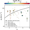 |
Fig. 5. Velocity dispersion of the ionised gas as a function of redshift. The dashed line shows the fit from Übler et al. (2019) for ionised gas at 0.6 < z < 2.6 extrapolated to higher redshifts, while the circles show results from a selection of ground-based IFU surveys in the near-infrared (Turner et al. 2017; Förster Schreiber et al. 2018) and the squares the results from ground-based near-infrared MOS data (the resolved and aligned sample of Price et al. 2020). The blue triangles show results from various studies with ALMA that measure the kinematics of the cold gas for massive, dusty star-forming galaxies (Neeleman et al. 2020; Rizzo et al. 2020; Fraternali et al. 2021; Lelli et al. 2021; Rizzo et al. 2021; Herrera-Camus et al. 2022; Parlanti et al. 2023). |
Extrapolating the fit by Übler et al. (2019) at z ∼ 1 − 3 to z ∼ 7 suggests that the ionised gas in galaxies is highly turbulent at early epochs. In contrast, we find that all objects lie well below this extrapolation, and instead have velocity dispersions that are approximately equal to the average dispersion at z ∼ 2 − 3. On the other hand, the typical stellar mass of our sample is substantially lower than the literature data (Fig. 2). If the velocity dispersion depends on stellar mass (as predicted by simulations, e.g., Pillepich et al. 2019), the ISM in these low-mass systems may still have a relatively high turbulence.
We also compared our results with studies that used ALMA to resolve galaxy kinematics at the same redshift as our sample (blue triangles; Neeleman et al. 2020; Rizzo et al. 2020, 2021; Fraternali et al. 2021; Lelli et al. 2021; Herrera-Camus et al. 2022; Parlanti et al. 2023). Although these objects lie at the same redshift, the measurements differ substantially: The galaxies observed with ALMA are often more massive (M* ≳ 1010 M⊙), and the observed emission lines tend to trace much colder gas. Interestingly, despite these differences, the ALMA-based velocity dispersions are very similar to our measurements of the ionised gas based on rest-frame optical emission lines. The reason might be that the effects of the higher mass and lower gas temperature on the velocity dispersion act in opposite directions. Observations of the same systems with both ALMA and JWST will be crucial to constrain these effects.
Next, we computed the ratio v/σ ≡ v(re)/σ0 and examined its dependence on redshift in Fig. 6 by comparing it with the same literature as mentioned previously. Studies around cosmic noon showed a clear, gradual decline in the degree of rotational support toward higher redshift. Based on these measurements, we may expect that none of the z > 5 galaxies are dominated by rotation (v/σ > 1). We find an interesting diversity in our sample, however, three objects of which have v/σ > 1 even at the highest redshifts (z ∼ 7). We discuss in Sect. 5 whether these objects may truly form cold rotating discs, or if they reflect velocity gradients within systems that are not virialised.
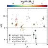 |
Fig. 6. Rotational support as a function of redshift, measured as the ratio of the velocity at the effective radius and the constant velocity dispersion: v(re)/σ0. Although studies based on ground-based near-infrared data (as described in Fig. 5) have found a clear, gradual decline in v/σ toward higher redshift, we find an interesting diversity among our sample of low-mass galaxies, with dynamically cold discs existing possibly as early as z ∼ 7. |
We again compared our sample with the ALMA-based studies, which are all rotation-dominated systems with relatively high v/σ ratios. Our sample shows greater diversity, which may be due to the fact that the gas tracers differ and the mass range probed is significantly different. The misalignment of some objects with the microshutters also may underestimate the intrinsic v/σ ratio of some systems. Larger samples are therefore required to fully understand the different kinematic properties of the gas phases traced with ALMA and JWST at high redshifts
Lastly, we revisit Sect. 2.2, where we described that for two out six objects the NIRCam image used as a prior in the emission line modelling predominantly traces stellar continuum emission instead of line emission. If the morphology of the emission line differs strongly from the continuum, this may bias the inferred kinematic parameters, especially if the galaxy is prolate instead of our assumed oblate thin-disc model. One of these two objects (JADES-NS-00016745; Fig. 3) has a major axis in the NIRCam image that is well-aligned with the microshutter, and we observe a strong velocity gradient in the 2D spectrum with only a small offset between the major axis PA from the imaging and the median of the posterior distribution of the PA (shown in Fig. 4). A prolate morphology is therefore highly unlikely for this object. The nature of the second object (JADES-NS-100016374) is more uncertain, as we only marginally detect rotation. If the kinematic major axis of the ionised gas differs strongly from the photometric major axis, the true rotational velocity and v/σ0 may be substantially higher than inferred with our modelling.
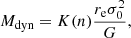
4.2. Comparing dynamical and stellar masses
We used the dynamical models to examine the mass budget of the galaxies. For a system in virial equilibrium, the dynamical mass enclosed within radius r is computed as
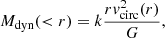 (3)
(3)
where vcirc is the circular velocity, k is the virial coefficient, and G is the gravitational constant. However, for comparison with the total stellar mass, we define a ‘total’ dynamical mass as described in Price et al. (2022),
 (4)
(4)
As we assumed a thin-disc model, we adopted ktot = 1.8, which is the virial coefficient for an oblate potential with q = 0.2 and n ∼ 1 − 4 (Price et al. 2022, Fig. 4). The true shape of the potential is poorly constrained, however, and this choice for ktot therefore introduces a systematic uncertainty in the dynamical mass estimates because ktot can vary by up to a factor of 2.
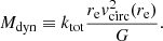
Following Burkert et al. (2010), we computed the circular velocity as
 (5)
(5)
which accounts for the effects of pressure gradients on the rotational velocity and depends on the disk scale length (rd). At the effective radius, the pressure correction term reduces to 2(re/rd) = 3.35. We note that for the one object with uncertain oblate or prolate morphology (Sect. 4.1), this calculation of vcirc may be incorrect. However, as discussed in Sect. 5.2, the inferred dynamical mass is likely less affected.
Next, we compared these total dynamical masses to the stellar masses. To estimate the stellar masses and SFRs, we performed SED modelling with the Bayesian fitting code BEAGLE (Chevallard & Charlot 2016) to the low-resolution prism spectra. The fits were run adopting a two-component star formation history consisting of a delayed exponential with current burst, a Chabrier (2003) initial mass function with an upper mass limit of 100 M⊙, and a Charlot & Fall (2000) dust-attenuation law assuming 40% of the dust in the diffuse ISM. We note that the 1D prism spectra were flux calibrated assuming a point-like morphology and without considering NIRCam photometry. Although this slit-loss correction approximately corrects for the variation in the PSF FWHM with wavelength, there is a systematic offset between the total flux of the object and the flux captured by the slit. We estimated this aperture correction using our modelling software and the morphology in the long-wavelength filter (F444W; measured with lenstronomy as described in Sect. 3.3), finding correction factors in the range 1.2 − 2.5, and we applied this to the stellar masses and SFRs. The inferred properties are presented in Appendix B, together with an example prism spectrum and SED model.
We compare the estimated dynamical and stellar masses in Fig. 7, and for reference, we plot the same ground-based near-infrared studies as in Figs. 5 and 6. As may be expected from the fact that Mdyn includes dark and baryonic mass, all objects in our sample have dynamical masses that exceed the estimated stellar masses. However, the difference between the two masses is much larger than in previous studies. It deviates by as much as a factor of 30 on average. Only Topping et al. (2022) have reported similarly large stellar-to-dynamical mass discrepancies at z ∼ 7, but for more massive galaxies and based on spatially integrated line-width measurements instead of spatially resolved dynamical modelling, as in this paper. We discuss the possible origins of this discrepancy between the stellar and dynamical masses in detail in Sect. 5.2.
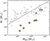 |
Fig. 7. Stellar mass versus dynamical mass (Eq. (4)) as inferred from the prism and high-resolution spectroscopy, respectively. The dashed line shows the one-to-one relation between the two masses. The data points from the literature (circles, squares) are as described in Fig. 5. As is to be expected, the dynamical masses are higher than the stellar masses for all objects in our sample. Surprisingly, however, the dynamical masses are substantially higher (up to a factor of ∼40), most likely indicating high gas masses or large systematic uncertainties in the stellar mass estimates. |
5. Discussion
These data and modelling have taken us to a very new regime of galaxy kinematics: low-mass galaxies at z > 5. Our modelling results are formally very well constrained, and the resulting parameter constraints (e.g., M* vs. Mdyn) at face value imply spectacular results. A look at Fig. 1 also makes it clear, however, that our simple symmetric models may not capture the complex geometry of the systems. Therefore, our results warrant and require careful discussion.
5.1. Clumpy cold discs or mergers?
Using a forward-modelling approach, we were able to separately constrain the morphology, velocity gradient, and intrinsic velocity dispersion for each JADES object. To do this, we assumed an underlying model of a thin rotating disc (Sect. 3.1). The velocity gradients measured in the context of our model suggest that the systems are dynamically relatively cold with higher than anticipated v/σ ratios (Fig. 6) based on an extrapolation of kinematic studies at z < 4.
However, both observations and theoretical models have suggested that the rate of (major) mergers rises rapidly toward z ∼ 6 (e.g., Rodriguez-Gomez et al. 2015; Bowler et al. 2017; Duncan et al. 2019; O’Leary et al. 2021). It is therefore likely that some objects in our sample are merging systems, or have recently merged with another galaxy. We indeed find complex (emission line) morphologies for several objects, most notably apparent in objects JADES-NS-00016745 and JADES-NS-20086025 (see Fig. 1), and Baker et al. (2023) showed that object JADES-NS-00047100 can be described by three separate morphological components. It is therefore possible that the rotational velocities inferred under the assumption of a virialised system may actually reflect the velocity offset between two (or more) objects or the velocity gradients induced by the gravitational interaction in a pre- or post-merger phase.
Observations, on the other hand, also show that high-redshift galaxies often contain large star-forming clumps, and that the overall clumpiness of galaxies increases toward higher redshifts and lower masses (e.g., Guo et al. 2015; Carniani et al. 2018; Zhang et al. 2019; Sattari et al. 2023). Importantly, these clumps do not necessarily lead to a globally unstable system and can be sustained within a rotationally-supported but warm disc (Förster Schreiber et al. 2011; Mandelker et al. 2014).
With the small angular scales (∼0.2″) and velocity differences (Δv ∼ 200 km s−1) involved for the systems studied in this paper, it is very difficult to distinguish between a merging system and star-forming clumps with ordered rotation. This degeneracy has been discussed extensively in the literature, although for lower redshifts and larger angular scales (e.g., Krajnović et al. 2006; Shapiro et al. 2008; Wisnioski et al. 2015; Rodrigues et al. 2017). Simons et al. (2019) used simulations of merging galaxies to construct mock observations and hence quantify the frequency with which these systems are misclassified as rotating discs, showing that misclassifications are very common (∼50%), unless very stringent disc-selection criteria are applied. Similarly, Hung et al. (2015, 2016) demonstrated that it becomes increasingly difficult to distinguish mergers from rotating systems toward later stages in the interaction between galaxies. On the other hand, Robertson et al. (2006) used hydrodynamical simulations to show that mergers between gas-rich systems can also lead to the formation of rotating discs with high angular momentum. Gravitational interaction between galaxies and the formation of rotating discs are thus not necessarily mutually exclusive, and the high gas fractions inferred in the next Sect. 5.2 are at face value consistent with the scenario proposed in these simulations.
Therefore, for any individual galaxy in our sample, we cannot definitively conclude whether it truly is a rotating disc or an ongoing merging system. Although the NIRSpec MOS data are unprecedented in depth, resolution, and sensitivity for galaxies at this mass and redshift, the objects are resolved by only a few resolution elements along a single spatial direction. Follow-up observations with the NIRSpec IFS mode can provide resolved 2D velocity field maps for these systems, which may then be compared against the disc-selection criteria of Wisnioski et al. (2015) and Simons et al. (2019) to improve the constraints on their dynamical states. However, the high-resolution NIRSpec IFS observations needed are not feasible for large samples of objects. It therefore seems inevitable at present to accept the fact that the nature of individual galaxies remains ambiguous. A statistical framework combining merger rates of galaxies and their observed emission line kinematics may provide a way forward to observationally constrain the settling of galaxies into cold discs at high redshifts, with number statistics that will be provided by upcoming surveys.
5.2. Uncertainties in the mass budget
We found a large discrepancy between the stellar and dynamical masses for the JADES objects. The dynamical mass presumably reflects the sum of the dark, stellar, and gas mass within the effective radius. It is therefore not unexpected that the dynamical masses are higher than the stellar masses. However, the magnitude of the mass discrepancy (more than an order of magnitude) is surprising because it is significantly higher than previous studies at lower redshifts at low mass (e.g., Maseda et al. 2013).
Considering the discussion of the previous section, we should first examine the robustness of our dynamical masses. To calculate the dynamical mass (Eq. (4)), we assumed that the galaxies are virialised; to compute the circular velocity, we assumed that the mass profile is approximately consistent with a rotating disc and exponential mass distribution. For the dispersion-dominated objects, the latter assumption may be problematic. When we instead assume a spherical mass distribution for these objects, we can follow the dynamical mass calculation for dispersion-supported systems by Cappellari et al. (2006),
 (6)
(6)
where the virial coefficient depends on the Sérsic index, K(n) = 8.87 − 0.831n + 0.0241n2. However, for the low Sérsic indices of our sample, K(n ∼ 1)∼8 and is therefore comparable to the coefficients that enter Eq. (4), as  . Similarly, in case of a prolate mass distribution, we would expect ktot ∼ 4 (Price et al. 2022) and
  . In other words, the dynamical mass would not be overestimated by much if systems were actually dispersion dominated. On the contrary, for the object in our sample with uncertain oblate or prolate morphology (Sect. 4.1), the rotational velocity might be underestimated, which would lead to an underestimation of the dynamical mass and stellar-to-dynamical mass discrepancy.
On the other hand, for the rotation-dominated objects, Mdyn will be dominated by the value of v(re). If this velocity does not reflect the rotational velocity of a virialised system but a velocity offset between two objects, then we cannot expect the dynamical mass estimate to be accurate. Both Simons et al. (2019) and Kohandel et al. (2019) explored the effects of incorrect physical and observational assumptions on the resulting vcirc and Mdyn estimates using mock observations of simulated galaxies. Simons et al. (2019) showed that for a merging system (noting that this is only a single simulation), the circular velocity is overestimated on average by a factor of ∼1.5 (∼0.15 dex), which translates into an overestimation of Mdyn by a factor of 2 (0.3 dex). Kohandel et al. (2019) showed that depending on the assumed inclination angle, Mdyn can be both under- and overestimated in the case of a merger, and they obtained a mass discrepancy of ∼ ± 0.3 dex for velocity offsets of the same magnitude as found in our sample. Together with the uncertainty in the virial coefficient (see Sect. 4.2), we therefore conclude that the dynamical masses may be overestimated by up to ∼0.3 − 0.6 dex, which cannot explain the large differences we find between the stellar and dynamical masses.
Crucially, we assumed above that the inferred gas kinematics are dominated by gravitational motions. If the velocity dispersions or velocity gradients are instead the result of non-gravitational motions, that is, turbulence and outflows due to stellar feedback, then the dynamical masses may be severely overestimated. As is discussed in great detail in Übler et al. (2019), based on theoretical models, the turbulence due to stellar feedback appears to be in the range of ∼10 − 20 km s−1 (Ostriker & Shetty 2011; Shetty & Ostriker 2012; Krumholz et al. 2018). This is significantly lower than the circular velocities measured for our sample and therefore cannot lead to a large bias in our dynamical masses.
Outflows, however, may form a larger source of uncertainty. We selected against objects in JADES with outflows as presented in Carniani et al. (2023), who measured outflow velocities vout > 200 km s−1. Lower outflow velocities are difficult to detect, but may still be present in our data. We therefore turned to observations of starburst galaxies at low redshift for comparison. Heckman et al. (2015) and Xu et al. (2022) detected outflows using UV metal absorption lines and demonstrated that the ratio vout/vcirc correlates with both the specific SFR (sSFR ≡ SFR/M*) and the SFR surface density (ΣSFR). Based on Fig. 10 of Xu et al. (2022) and the fact that for our sample, sSFR ∼ 10−8 yr−1 and ΣSFR ∼ 10 M⊙ yr−1 kpc−2, we estimate vout/vcirc ∼ 3. This would imply an overestimation of the circular velocity by a factor of 3 or a factor of 10 in the dynamical mass. However, it is unclear whether the outflowing gas traced by the rest-frame UV absorption lines is also traced by the rest-frame optical emission lines, and how this in turn would translate into the uncertainty on the dynamical mass. For example, Erb et al. (2006) found no correlation between the Hα line width (and hence the dynamical mass) and galactic outflow velocities measured from rest-frame UV absorption lines for more massive star-forming galaxies at z ∼ 2.
If the dynamical mass is robust (at the level of a factor of 2), we should turn our attention to the other mass components that contribute to the total mass budget. An obvious component not discussed so far is the gas mass. Both observational and theoretical studies have shown that it is important to take the gas content into account (Price et al. 2016; Wuyts et al. 2016) because the typical gas fraction rises rapidly toward higher redshift and lower masses (for a review, see Tacconi et al. 2020). We estimated the gas masses of our sample based on the SFRs obtained from the SED modelling to the prism spectroscopy. We used the inverse of the Kennicutt (1998) relation between gas surface mass density (Σgas) and SFR to infer the total gas mass. Although calibrated only at low redshifts, this likely provides a reasonable order-of-magnitude estimate for the high SFR surface densities of our sample (Daddi et al. 2010; Kennicutt & Evans 2012).
From this, we find gas masses of about Mgas ∼ 109 M⊙ with an average ratio ⟨Mgas/M*⟩∼10. We can now compare these gas masses and resulting baryonic masses (Mbar ≡ M* + Mgas) to the dynamical masses in Fig. 8. Although the gas mass is higher than the stellar mass (fgas ≡ Mgas/Mbar ∼ 0.90; consistent with measurements of more massive galaxies at z ∼ 7 from Heintz et al. 2022), a discrepancy of approximately a factor of 3 − 4 between the baryonic and dynamical mass remains for all but one object. Our estimate of the gas masses carries a systematic uncertainty because it assumes, for instance, a constant star formation efficiency. Price et al. (2020) showed that a different estimator for the gas mass (following Tacconi et al. 2018) results in a mean gas mass difference of only 0.13 dex for a sample of more massive galaxies at cosmic noon. The same gas-scaling relations are poorly, if at all, constrained at z ∼ 6 in the stellar mass regime considered in this work, and we therefore cannot make the same comparison for our sample. To increase the gas masses and make the baryonic masses consistent with the dynamical masses would, however, require a decrease of a factor of ∼3 in the star formation efficiency for the majority of our sample. However, Pillepich et al. (2019) showed that in the cosmological simulation TNG50, the gas fraction in low-mass galaxies (M* ∼ 109) increases rapidly with redshift up to z ∼ 3 − 4, but then appears to flatten at higher redshifts with Mgas/Mdyn ∼ 0.2. Further observations as well as simulated data at even lower stellar masses and higher redshifts will be necessary to constrain the gas masses for objects similar to the JADES sample.
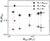 |
Fig. 8. Baryonic, stellar, and gas masses (estimated using the relation between ΣSFR and Σgas from Kennicutt 1998) as fractions of the dynamical mass. We find that the gas mass, and hence the baryonic mass, is approximately one order of magnitude higher than the stellar mass. Although the inclusion of the gas component reduces the large discrepancy in mass found in Fig. 7, the difference of a factor of 3 − 4 between the dynamical and baryonic mass still remains for all but one object. |
Importantly, the stellar masses may also be affected by systematic uncertainties. The low-resolution spectroscopy spans a broad wavelength range (1 − 5 μm), probing the rest-frame UV to optical for all objects, and therefore, it provides good constraints on the recent star formation history (SFH). However, these measurements may be affected by an outshining effect, in which a young star-forming population dominates the SED, making it almost impossible to detect an underlying population of older stars at rest-frame optical wavelengths (e.g., Maraston et al. 2010; Pforr et al. 2012; Sorba & Sawicki 2018; Giménez-Arteaga et al. 2023; Tacchella et al. 2023; Whitler et al. 2023). This is especially relevant for our sample because we selected bright emission lines to perform our dynamical modelling, and these lines tend to have high equivalent widths. Using mock observations of cosmological simulations, Narayanan et al. (2024) showed that the outshining effect may underestimate the stellar masses by 0.1 − 1.0 dex at z ∼ 7 depending on the selected prior for the SFH. This means that the possible severe underestimate of the stellar mass is the most problematic potential source of systematic errors in our mass budget. Imaging at longer wavelengths with JWST/MIRI and spatially resolved SED fitting may offer improvements in the stellar mass estimates in the future (e.g., Abdurro’uf et al. 2023; Giménez-Arteaga et al. 2023; Pérez-González et al. 2023). We note, however, that even this effect would have little effect in the regime where Mdyn is 30 × M*.
In summary, a number of systematic effects may contribute to the large discrepancy of a factor of 30 between the stellar and dynamical masses for this low-mass, high-redshift sample. We argue that the dynamical masses are relatively well constrained, with an uncertainty of 0.3 − 0.6 dex at most, even in the case of an ongoing merger, although we cannot rule out a bias in some of the dynamical mass measurements due to galactic-scale outflows. Clearly, a substantial amount of gas must be present in these highly star-forming galaxies, and we estimate that this can account for ∼1 dex in the discrepancy of stellar to dynamical mass. Although the gas masses are uncertain and the scaling relations between SFR and gas surface densities have significant scatter, we consider it unlikely that the gas masses are underestimated by a large factor for all objects in our sample. This leaves the possibility that the stellar masses may instead be significantly underestimated because we lack constraints at longer rest-frame wavelengths where an older stellar population may be measurable.
In this discussion, we have neglected one mass component thus far: the dark matter. On the small spatial scales probed (∼1 kpc), this may not appear to be a dominant factor in the mass budget, particularly as multiple studies have shown a rapid increase in the central baryon fraction toward higher redshifts (e.g., van Dokkum et al. 2015; Price et al. 2016; Wuyts et al. 2016; Genzel et al. 2017, 2020). However, it is interesting to consider a situation with significant dark matter within the effective radii at these redshifts. Within the ΛCDM cosmological model, dark matter dominates the mass content of the Universe. Under hierarchical structure formation, small dark matter haloes form first, whereas stars only form after the gas within those haloes has cooled sufficiently, subsequently growing into galaxies through accretion (cold gas streams, mergers; e.g., White & Rees 1978; Dekel et al. 2009a; Oser et al. 2010). In this scenario, it may be possible that very young galaxies are dominated by dark matter even in the central regions because the baryonic mass is still being assembled. This is of particular interest because galaxies in the stellar mass regime probed in this paper (∼108 M⊙) may be the progenitors of galaxies of M* ∼ 1011 M⊙ at z = 0 (Moster et al. 2018; Behroozi et al. 2019), which have baryon-dominated centres. As the aforementioned observations at cosmic noon are typically also of more massive galaxies (M* ∼ 1010 − 11 M⊙), the difference in the central baryon fractions between our work and measurements at cosmic noon may therefore not differ, but reflect the time evolution in the distribution of dark and baryonic mass as galaxies grow and assemble their stellar mass. We explore this idea further using cosmological simulations in de Graaff et al. (in prep.). However, a definitive conclusion whether this scenario may apply to the JADES galaxies will require a thorough understanding of the systematic uncertainties on the different mass components.
6. Conclusions
We used the JADES spectroscopic sample in GOODS-S to select six targets at z = 5.5 − 7.4 that are spatially extended in NIRCam imaging, and for which high-resolution (R ∼ 2700) spectroscopy was obtained with the NIRSpec MSA. We showed that these galaxies lie in a previously unprobed part of parameter space: not only because of their high redshifts, but also because of their small sizes (∼1 kpc) and low stellar masses (M* ∼ 108 M⊙). The high-resolution spectra reveal rest-frame optical emission lines ([OIII] and Hα) that are broadened and have spatial velocity gradients.
To extract the dynamical properties, we modelled the objects as thin but warm rotating discs. We described a novel forward-modelling software to account for several complexities of data taken with the NIRSpec instrument: the PSF, shutter geometry and bar shadows, and pixellation. Using NIRCam imaging as a prior on the emission line morphology, we were able to constrain the rotational velocities and velocity dispersions of the objects in our sample, and hence, we were also able to estimate the dynamical masses. Our findings can be summarised as follows.
-
The objects in our sample are small (re ∼ 0.5 − 2 kpc), have a low stellar mass (M* ∼ 107.5 − 8.9), and modest star formation rates (SFR ∼ 2 − 20 M⊙ yr−1), which we inferred from SED modelling to low-resolution NIRSpec spectroscopy. The gas masses implied by the SFRs are ten times higher on average than the stellar masses.
-
We find intrinsic velocity dispersions in the range σ0 ∼ 30 − 70 km s−1, which is consistent with studies reporting the velocity dispersions of more massive galaxies at cosmic noon.
-
Three out of six objects show significant spatial velocity gradients, resulting in v/σ ∼ 1 − 6. Under the assumption of our thin-disc model, this implies that the high-redshift objects are rotation-dominated discs. However, we cannot rule out the possibility that the detected velocity gradients reflect velocity offsets between interacting galaxies.
-
The comparison between the dynamical and stellar masses revealed a surprising discrepancy of a factor of 10 − 40. After accounting for the high gas masses, the dynamical masses still remain higher than the baryonic masses by a factor of ∼3.
-
We argue that the dynamical masses are robust within a factor of 2 − 4 even in the case of an ongoing merger. Only the presence of outflows, if these were to dominate the observed emission line kinematics, can substantially lower the inferred dynamical masses. However, the baryonic-to-dynamical mass discrepancy might also imply that the centres of these objects are dominated by dark matter. Moreover, there are large systematic uncertainties on the stellar and gas masses. The baryonic masses can be reconciled with the dynamical masses if the star formation efficiency in these objects is lower by a factor of 3 than initially assumed.
Our work provides a first demonstration of the powerful capabilities of the NIRSpec MOS mode to perform spatially and spectrally resolved analyses. Crucially, this enables the study of galaxy kinematics in a highly efficient manner because a single observation can probe a wide range in redshift, mass, and SFR. With larger spectroscopic samples using the high-resolution MOS mode currently being acquired, JWST NIRSpec will in the near-future allow statistical analyses of the origins and settling of disc galaxies in the early Universe.
Software, reference data (PSF models, trace models) and installation instructions can be found here: https://github.com/annadeg/jwst-msafit
For a comprehensive technical description of NIRSpec, we refer the reader to Jakobsen et al. (2022) and Ferruit et al. (2022).
The IPC kernels are publicly available on the JDox: https://jwst-docs.stsci.edu/jwst-near-infrared-spectrograph/nirspec-instrumentation/nirspec-detectors/nirspec-detector-performance
https://jwst-docs.stsci.edu/jwst-near-infrared-spectrograph/nirspec-instrumentation/nirspec-dispersers-and-filters
Acknowledgments
AdG thanks M. Fouesneau and I. Momcheva for their valuable feedback during the development of msafit, and J. Davies for helpful discussions on JWST and NIRSpec data. This research makes use of ESA Datalabs (datalabs.esa.int), an initiative by ESA’s Data Science and Archives Division in the Science and Operations Department, Directorate of Science. This research made use of POPPY, an open-source optical propagation Python package originally developed for the James Webb Space Telescope project (Perrin et al. 2012). SC acknowledges support by European Union’s HE ERC Starting Grant No. 101040227 – WINGS. ECL acknowledges support of an STFC Webb Fellowship (ST/W001438/1) RM and WB acknowledge support by the Science and Technology Facilities Council (STFC), by the ERC through Advanced Grant 695671 “QUENCH”. RM also acknowledges support by the UKRI Frontier Research grant RISEandFALL and funding from a research professorship from the Royal Society. AJB, AJC, JC & GCJ acknowledge funding from the “FirstGalaxies” Advanced Grant from the European Research Council (ERC) under the European Union’s Horizon 2020 research and innovation programme (Grant agreement No. 789056). SA acknowledges support from Grant PID2021-127718NB-I00 funded by the Spanish Ministry of Science and Innovation/State Agency of Research (MICIN/AEI/ 10.13039/501100011033). HÜ gratefully acknowledges support by the Isaac Newton Trust and by the Kavli Foundation through a Newton-Kavli Junior Fellowship. DJE is supported as a Simons Investigator. DJE, BJJ and CNAW are supported by a JWST/NIRCam contract to the University of Arizona, NAS5-02015. BER acknowledges support from the NIRCam Science Team contract to the University of Arizona, NAS5-02015. The research of CCW is supported by NOIRLab, which is managed by the Association of Universities for Research in Astronomy (AURA) under a cooperative agreement with the National Science Foundation. KB acknowledges support from the Australian Research Council Centre of Excellence for All Sky Astrophysics in 3 Dimensions (ASTRO 3D), through project number CE170100013. RH acknowledges funding provided by the Johns Hopkins University, Institute for Data Intensive Engineering and Science (IDIES).
References
- Abdurro’uf, Coe, D., Jung, I., et al. 2023, ApJ, 945, 117 [CrossRef] [Google Scholar]
- Alves de Oliveira, C., Lützgendorf, N., Zeidler, P., et al. 2022, SPIE Conf. Ser., 12180, 121803S [NASA ADS] [Google Scholar]
- Baker, W. M., Tacchella, S., Johnson, B. D., et al. 2023, Nat. Astron., submitted, [arXiv:2306.02472] [Google Scholar]
- Behroozi, P., Wechsler, R. H., Hearin, A. P., & Conroy, C. 2019, MNRAS, 488, 3143 [NASA ADS] [CrossRef] [Google Scholar]
- Birrer, S., & Amara, A. 2018, Phys. Dark Universe, 22, 189 [NASA ADS] [CrossRef] [Google Scholar]
- Birrer, S., Shajib, A., Gilman, D., et al. 2021, J. Open Source Software, 6, 3283 [NASA ADS] [CrossRef] [Google Scholar]
- Böker, T., Arribas, S., Lützgendorf, N., et al. 2022, A&A, 661, A82 [NASA ADS] [CrossRef] [EDP Sciences] [Google Scholar]
- Böker, T., Beck, T. L., Birkmann, S. M., et al. 2023, PASP, 135, 038001 [CrossRef] [Google Scholar]
- Bowler, R. A. A., Dunlop, J. S., McLure, R. J., & McLeod, D. J. 2017, MNRAS, 466, 3612 [NASA ADS] [CrossRef] [Google Scholar]
- Bunker, A. J., Cameron, A. J., Curtis-Lake, E., et al. 2023, A&A, submitted, [arXiv:2306.02467] [Google Scholar]
- Burkert, A., Genzel, R., Bouché, N., et al. 2010, ApJ, 725, 2324 [Google Scholar]
- Cappellari, M. 2016, ARA&A, 54, 597 [Google Scholar]
- Cappellari, M., Bacon, R., Bureau, M., et al. 2006, MNRAS, 366, 1126 [Google Scholar]
- Carniani, S., Maiolino, R., Amorin, R., et al. 2018, MNRAS, 478, 1170 [NASA ADS] [CrossRef] [Google Scholar]
- Carniani, S., Venturi, G., Parlanti, E., et al. 2023, A&A, in press, [arXiv:2306.11801] [Google Scholar]
- Ceverino, D., Dekel, A., Mandelker, N., et al. 2012, MNRAS, 420, 3490 [NASA ADS] [CrossRef] [Google Scholar]
- Chabrier, G. 2003, ApJ, 586, L133 [NASA ADS] [CrossRef] [Google Scholar]
- Charlot, S., & Fall, S. M. 2000, ApJ, 539, 718 [Google Scholar]
- Chevallard, J., & Charlot, S. 2016, MNRAS, 462, 1415 [NASA ADS] [CrossRef] [Google Scholar]
- Courteau, S. 1997, AJ, 114, 2402 [Google Scholar]
- Curtis-Lake, E., Carniani, S., Cameron, A., et al. 2023, Nat. Astron., 7, 622 [NASA ADS] [CrossRef] [Google Scholar]
- Daddi, E., Elbaz, D., Walter, F., et al. 2010, ApJ, 714, L118 [NASA ADS] [CrossRef] [Google Scholar]
- Dekel, A., Birnboim, Y., Engel, G., et al. 2009a, Nature, 457, 451 [Google Scholar]
- Dekel, A., Sari, R., & Ceverino, D. 2009b, ApJ, 703, 785 [Google Scholar]
- Dorner, B., Giardino, G., Ferruit, P., et al. 2016, A&A, 592, A113 [NASA ADS] [CrossRef] [EDP Sciences] [Google Scholar]
- Duncan, K., Conselice, C. J., Mundy, C., et al. 2019, ApJ, 876, 110 [NASA ADS] [CrossRef] [Google Scholar]
- Eisenstein, D. J., Willott, C., Alberts, S., et al. 2023, ApJS, submitted, [arXiv:2306.02465] [Google Scholar]
- Erb, D. K., Steidel, C. C., Shapley, A. E., et al. 2006, ApJ, 646, 107 [NASA ADS] [CrossRef] [Google Scholar]
- Falcón-Barroso, J., van de Ven, G., Lyubenova, M., et al. 2019, A&A, 632, A59 [Google Scholar]
- Ferruit, P., Jakobsen, P., Giardino, G., et al. 2022, A&A, 661, A81 [NASA ADS] [CrossRef] [EDP Sciences] [Google Scholar]
- Foreman-Mackey, D., Hogg, D. W., Lang, D., & Goodman, J. 2013, PASP, 125, 306 [Google Scholar]
- Förster Schreiber, N. M., & Wuyts, S. 2020, ARA&A, 58, 661 [Google Scholar]
- Förster Schreiber, N. M., Shapley, A. E., Erb, D. K., et al. 2011, ApJ, 731, 65 [CrossRef] [Google Scholar]
- Förster Schreiber, N. M., Renzini, A., Mancini, C., et al. 2018, ApJS, 238, 21 [Google Scholar]
- Fraternali, F., Karim, A., Magnelli, B., et al. 2021, A&A, 647, A194 [NASA ADS] [CrossRef] [EDP Sciences] [Google Scholar]
- Gardner, J. P., Mather, J. C., Abbott, R., et al. 2023, PASP, 135, 068001 [NASA ADS] [CrossRef] [Google Scholar]
- Genel, S., Dekel, A., & Cacciato, M. 2012, MNRAS, 425, 788 [CrossRef] [Google Scholar]
- Genzel, R., Förster Schreiber, N. M., Übler, H., et al. 2017, Nature, 543, 397 [Google Scholar]
- Genzel, R., Price, S. H., Übler, H., et al. 2020, ApJ, 902, 98 [NASA ADS] [CrossRef] [Google Scholar]
- Giardino, G., Luetzgendorf, N., Ferruit, P., et al. 2016, SPIE Conf. Ser., 9904, 990445 [NASA ADS] [Google Scholar]
- Giardino, G., Ferruit, P., Chevallard, J., et al. 2019, in Astronomical Data Analysis Software and Systems XXVII, eds. P. J. Teuben, M. W. Pound, B. A. Thomas, & E. M. Warner, ASP Conf. Ser., 523, 645 [NASA ADS] [Google Scholar]
- Giménez-Arteaga, C., Oesch, P. A., Brammer, G. B., et al. 2023, ApJ, 948, 126 [CrossRef] [Google Scholar]
- Guo, Y., Ferguson, H. C., Bell, E. F., et al. 2015, ApJ, 800, 39 [NASA ADS] [CrossRef] [Google Scholar]
- Heckman, T. M., Alexandroff, R. M., Borthakur, S., Overzier, R., & Leitherer, C. 2015, ApJ, 809, 147 [Google Scholar]
- Heintz, K. E., Oesch, P. A., Aravena, M., et al. 2022, ApJ, 934, L27 [NASA ADS] [CrossRef] [Google Scholar]
- Herrera-Camus, R., Förster Schreiber, N. M., Price, S. H., et al. 2022, A&A, 665, L8 [NASA ADS] [CrossRef] [EDP Sciences] [Google Scholar]
- Hung, C.-L., Rich, J. A., Yuan, T., et al. 2015, ApJ, 803, 62 [Google Scholar]
- Hung, C.-L., Hayward, C. C., Smith, H. A., et al. 2016, ApJ, 816, 99 [NASA ADS] [CrossRef] [Google Scholar]
- Jakobsen, P., Ferruit, P., Alves de Oliveira, C., et al. 2022, A&A, 661, A80 [NASA ADS] [CrossRef] [EDP Sciences] [Google Scholar]
- Johnson, B. D. 2019, SEDPY: Modules for storing and operating on astronomical source spectral energy distribution, Astrophysics Source Code Library [record ascl:1905.026] [Google Scholar]
- Jones, G. C., Vergani, D., Romano, M., et al. 2021, MNRAS, 507, 3540 [NASA ADS] [CrossRef] [Google Scholar]
- Kennicutt, R. C., Jr 1998, ARA&A, 36, 189 [NASA ADS] [CrossRef] [Google Scholar]
- Kennicutt, R. C., & Evans, N. J. 2012, ARA&A, 50, 531 [NASA ADS] [CrossRef] [Google Scholar]
- Kohandel, M., Pallottini, A., Ferrara, A., et al. 2019, MNRAS, 487, 3007 [NASA ADS] [CrossRef] [Google Scholar]
- Krajnović, D., Cappellari, M., de Zeeuw, P. T., & Copin, Y. 2006, MNRAS, 366, 787 [Google Scholar]
- Krumholz, M. R., Burkhart, B., Forbes, J. C., & Crocker, R. M. 2018, MNRAS, 477, 2716 [CrossRef] [Google Scholar]
- Lelli, F., Di Teodoro, E. M., Fraternali, F., et al. 2021, Science, 371, 713 [Google Scholar]
- Lützgendorf, N., Giardino, G., Alves de Oliveira, C., et al. 2022, SPIE Conf. Ser., 12180, 121800Y [Google Scholar]
- Mandelker, N., Dekel, A., Ceverino, D., et al. 2014, MNRAS, 443, 3675 [NASA ADS] [CrossRef] [Google Scholar]
- Maraston, C., Pforr, J., Renzini, A., et al. 2010, MNRAS, 407, 830 [NASA ADS] [CrossRef] [Google Scholar]
- Maseda, M. V., van der Wel, A., da Cunha, E., et al. 2013, ApJ, 778, L22 [NASA ADS] [CrossRef] [Google Scholar]
- Moster, B. P., Naab, T., & White, S. D. M. 2018, MNRAS, 477, 1822 [Google Scholar]
- Narayanan, D., Lower, S., Torrey, P., et al. 2024, ApJ, 961, 73 [NASA ADS] [CrossRef] [Google Scholar]
- Neeleman, M., Prochaska, J. X., Kanekar, N., & Rafelski, M. 2020, Nature, 581, 269 [Google Scholar]
- Newman, A. B., Belli, S., Ellis, R. S., & Patel, S. G. 2018, ApJ, 862, 126 [NASA ADS] [CrossRef] [Google Scholar]
- Nidever, D. L., Gilbert, K., Tollerud, E., et al. 2023, Early Disk-Galaxy Formation from JWST to the Milky Way, eds. F. Tabatabaei, B. Barbuy,& Y.-S. Ting, Proc. Int. Astron. Union, 377, 115 [NASA ADS] [Google Scholar]
- Oesch, P. A., Brammer, G., Naidu, R. P., et al. 2023, MNRAS, 525, 2864 [NASA ADS] [CrossRef] [Google Scholar]
- O’Leary, J. A., Moster, B. P., Naab, T., & Somerville, R. S. 2021, MNRAS, 501, 3215 [Google Scholar]
- Oser, L., Ostriker, J. P., Naab, T., Johansson, P. H., & Burkert, A. 2010, ApJ, 725, 2312 [Google Scholar]
- Ostriker, E. C., & Shetty, R. 2011, ApJ, 731, 41 [Google Scholar]
- Parlanti, E., Carniani, S., Pallottini, A., et al. 2023, A&A, 673, A153 [NASA ADS] [CrossRef] [EDP Sciences] [Google Scholar]
- Pérez-González, P. G., Barro, G., Annunziatella, M., et al. 2023, ApJ, 946, L16 [CrossRef] [Google Scholar]
- Perrin, M. D., Soummer, R., Elliott, E. M., Lallo, M. D., & Sivaramakrishnan, A. 2012, SPIE Conf. Ser., 8442, 84423D [NASA ADS] [Google Scholar]
- Pforr, J., Maraston, C., & Tonini, C. 2012, MNRAS, 422, 3285 [NASA ADS] [CrossRef] [Google Scholar]
- Pillepich, A., Nelson, D., Springel, V., et al. 2019, MNRAS, 490, 3196 [Google Scholar]
- Piquéras, L., Legay, P. J., Legros, E., et al. 2008, SPIE Conf. Ser., 7017, 70170Z [Google Scholar]
- Piquéras, L., Legros, E., Pons, A., et al. 2010, SPIE Conf. Ser., 7738, 773812 [Google Scholar]
- Pope, A., McKinney, J., Kamieneski, P., et al. 2023, ApJ, 951, L46 [NASA ADS] [CrossRef] [Google Scholar]
- Price, S. H., Kriek, M., Shapley, A. E., et al. 2016, ApJ, 819, 80 [Google Scholar]
- Price, S. H., Kriek, M., Barro, G., et al. 2020, ApJ, 894, 91 [NASA ADS] [CrossRef] [Google Scholar]
- Price, S. H., Übler, H., Förster Schreiber, N. M., et al. 2022, A&A, 665, A159 [NASA ADS] [CrossRef] [EDP Sciences] [Google Scholar]
- Rieke, M. J., Kelly, D. M., Misselt, K., et al. 2023a, PASP, 135, 028001a [NASA ADS] [CrossRef] [Google Scholar]
- Rieke, M. J., Robertson, B., Tacchella, S., et al. 2023b, ApJS, 269, 16 [NASA ADS] [CrossRef] [Google Scholar]
- Rigby, J., Perrin, M., McElwain, M., et al. 2023, PASP, 135, 048001 [NASA ADS] [CrossRef] [Google Scholar]
- Rizzo, F., Vegetti, S., Powell, D., et al. 2020, Nature, 584, 201 [Google Scholar]
- Rizzo, F., Vegetti, S., Fraternali, F., Stacey, H. R., & Powell, D. 2021, MNRAS, 507, 3952 [NASA ADS] [CrossRef] [Google Scholar]
- Rizzo, F., Roman-Oliveira, F., Fraternali, F., et al. 2023, A&A, 679, A129 [NASA ADS] [CrossRef] [EDP Sciences] [Google Scholar]
- Robertson, B., Bullock, J. S., Cox, T. J., et al. 2006, ApJ, 645, 986 [NASA ADS] [CrossRef] [Google Scholar]
- Rodrigues, M., Hammer, F., Flores, H., Puech, M., & Athanassoula, E. 2017, MNRAS, 465, 1157 [NASA ADS] [CrossRef] [Google Scholar]
- Rodriguez-Gomez, V., Genel, S., Vogelsberger, M., et al. 2015, MNRAS, 449, 49 [Google Scholar]
- Sattari, Z., Mobasher, B., Chartab, N., et al. 2023, ApJ, 951, 147 [NASA ADS] [CrossRef] [Google Scholar]
- Sérsic, J. L. 1968, Atlas de Galaxias Australes (Cordoba, Argentina: Observatorio Astronomico) [Google Scholar]
- Shapiro, K. L., Genzel, R., Förster Schreiber, N. M., et al. 2008, ApJ, 682, 231 [NASA ADS] [CrossRef] [Google Scholar]
- Shetty, R., & Ostriker, E. C. 2012, ApJ, 754, 2 [NASA ADS] [CrossRef] [Google Scholar]
- Simons, R. C., Kassin, S. A., Weiner, B. J., et al. 2017, ApJ, 843, 46 [Google Scholar]
- Simons, R. C., Kassin, S. A., Snyder, G. F., et al. 2019, ApJ, 874, 59 [Google Scholar]
- Sorba, R., & Sawicki, M. 2018, MNRAS, 476, 1532 [NASA ADS] [CrossRef] [Google Scholar]
- Stott, J. P., Swinbank, A. M., Johnson, H. L., et al. 2016, MNRAS, 457, 1888 [Google Scholar]
- Suess, K. A., Williams, C. C., Robertson, B., et al. 2023, ApJ, 956, L42 [CrossRef] [Google Scholar]
- Tacchella, S., Johnson, B. D., Robertson, B. E., et al. 2023, MNRAS, 522, 6236 [NASA ADS] [CrossRef] [Google Scholar]
- Tacconi, L. J., Genzel, R., Saintonge, A., et al. 2018, ApJ, 853, 179 [Google Scholar]
- Tacconi, L. J., Genzel, R., & Sternberg, A. 2020, ARA&A, 58, 157 [NASA ADS] [CrossRef] [Google Scholar]
- Topping, M. W., Stark, D. P., Endsley, R., et al. 2022, MNRAS, 516, 975 [NASA ADS] [CrossRef] [Google Scholar]
- Turner, O. J., Cirasuolo, M., Harrison, C. M., et al. 2017, MNRAS, 471, 1280 [Google Scholar]
- Übler, H., Genzel, R., Wisnioski, E., et al. 2019, ApJ, 880, 48 [Google Scholar]
- van de Sande, J., Scott, N., Bland-Hawthorn, J., et al. 2018, Nat. Astron., 2, 483 [Google Scholar]
- van der Wel, A., Bell, E. F., Häussler, B., et al. 2012, ApJS, 203, 24 [NASA ADS] [CrossRef] [Google Scholar]
- van der Wel, A., Chang, Y.-Y., Bell, E. F., et al. 2014, ApJ, 792, L6 [NASA ADS] [CrossRef] [Google Scholar]
- van Dokkum, P. G., Nelson, E. J., Franx, M., et al. 2015, ApJ, 813, 23 [NASA ADS] [CrossRef] [Google Scholar]
- van Houdt, J., van der Wel, A., Bezanson, R., et al. 2021, ApJ, 923, 11 [CrossRef] [Google Scholar]
- Whitaker, K. E., Franx, M., Leja, J., et al. 2014, ApJ, 795, 104 [NASA ADS] [CrossRef] [Google Scholar]
- White, S. D. M., & Rees, M. J. 1978, MNRAS, 183, 341 [Google Scholar]
- Whitler, L., Stark, D. P., Endsley, R., et al. 2023, MNRAS, 519, 5859 [NASA ADS] [CrossRef] [Google Scholar]
- Wisnioski, E., Förster Schreiber, N. M., Wuyts, S., et al. 2015, ApJ, 799, 209 [Google Scholar]
- Wisnioski, E., Förster Schreiber, N. M., Fossati, M., et al. 2019, ApJ, 886, 124 [Google Scholar]
- Wuyts, S., Förster Schreiber, N. M., Wisnioski, E., et al. 2016, ApJ, 831, 149 [Google Scholar]
- Xu, X., Heckman, T., Henry, A., et al. 2022, ApJ, 933, 222 [NASA ADS] [CrossRef] [Google Scholar]
- Zhang, H., Primack, J. R., Faber, S. M., et al. 2019, MNRAS, 484, 5170 [NASA ADS] [CrossRef] [Google Scholar]
Appendix A: NIRSpec resolution
The instrument resolution for NIRSpec provided in the online JWST user documentation (JDox) provides a pre-launch estimate of the 1D instrument LSF for a uniformly illuminated slit4. However, as we already account for the source morphology in our modelling, the point source resolution is relevant in our work. To provide insight into our model PSFs, which are 2D images, we used our modelling software to estimate the 1D resolution as a function of wavelength for a point source.
To do this, we set up a model cube I(x, y, λ) following the procedure described in Section 3, but for a point source morphology instead of a Sérsic profile. We placed the point source in the centre of the shutter and used a central shutter (sij = (185, 85)) of the fourth quadrant of the MSA. We applied a sparse wavelength sampling of Δλ = 0.2 μm across 2.7 < λ < 5.3 μm to avoid overlapping and to speed up the computation. We then propagated this model onto the detector plane and extracted a 1D spectrum. By modelling the resulting emission lines at the known input wavelengths as a series of single Gaussians with variable width and amplitude, we derived the LSF for a point source.
We show the resulting resolution and LSF for a point source for the G395H grating in Fig. A.1. The point source resolution of NIRSpec (dashed lines) is substantially higher than the estimate for a uniformly illuminated slit (solid lines). In the right panel, we show the ratio of the two as a function of wavelength: At shorter wavelengths, the resolution differs by nearly a factor of 2. At longer wavelengths, this discrepancy in resolution gradually decreases because the ratio of the spatial PSF FWHM and the slit width increases with wavelength (i.e. the spatial PSF becomes broader and therefore closer to the approximation of a uniform flux distribution). We caution that this LSF cannot be applied directly to 1D rectified, extracted, and combined spectra from real observations because it does not include broadening that is usually introduced by the reduction pipeline when resampling and combining data from multiple exposures. In principle, our model detectors can be propagated through any reduction pipeline to estimate this additional broadening, and we investigate these effects in more detail in de Graaff et al. (in prep).
Moreover, as noted in Section 3.2, we emphasise that the PSF models used in our forward modelling rely partially on reference files that were created pre-launch, which likely leads to a systematic uncertainty in the FWHM. A small number of calibration programs that aim to characterise the PSF have been executed, which we discuss as follows.
For the MSA, a single standard star was observed in the prism mode within the central shutter of each quadrant to obtain the spatial PSF (programme 1128). Similarly, for the fixed slit (FS; programmes 1128, 1487), a standard star was observed at different intraslit positions. These data are primarily suited and used to estimate path losses. Because the PSF is highly undersampled (pixels of 0.1″ vs. an FWHM ∼0.03 − 0.16″ if the PSF is diffraction limited), and only one object was observed, it is extremely challenging in practice to extract a robust spatial profile from these data. Jakobsen et al. (2022) reported that the spatial PSF of NIRSpec is diffraction limited beyond 3.2 μm and is therefore similar to the NIRCam PSF at long wavelengths. All emission lines considered in this paper are at λ > 3.4 μm and in this diffraction-limited regime.
We assessed the quality of the spatial (i.e. cross-dispersion) direction of our PSF models by comparing the half-light radii inferred from our modelling to the NIRCam images and those inferred from the spectral modelling. Although we have set a prior based on the NIRCam morphological information to model the spectra, the widths of the priors are sufficiently broad. Therefore, in the case of a substantial deviation between the true PSF and our model PSF, we would expect to find a systematic difference in the half-light radii between the two measurements, particularly for the objects that are compact (< 0.15″; Table 2). We find a median difference of only ∼10%, however, with the spectral fits indicating slightly larger sizes. This small bias may also be a physical effect because the NIRCam images contain flux from both the stellar continuum and emission lines.
For the dispersion direction, the only available calibration data are of a distant planetary nebula (PN), which was observed in the MOS and FS modes (programmes 1125, 1492). Apart from the fact that this object may not be a true point source, the undersampling again is the dominant issue in calibrating the broadening in the dispersion direction. Similar to the spatial PSF, the LSF is highly undersampled for a point source (FWHM∼1 pix). The fact that the PN spectrum shows only few (about ten) narrow emission lines across 3 − 5 μm and that only a single object was observed means that constraining the spectral broadening is a major outstanding challenge.
However, our modelling software also makes predictions for other NIRSpec dispersers. The preliminary analysis by Nidever et al. (2023) is particularly relevant. They observed ∼100 red giant stars in M31 with the G140H grating (programme 2609). These spectra show many narrow absorption line features at high S/N, thereby enabling an empirical reconstruction of the LSF in spite of the undersampling issues. Nidever et al. (2023) found that for the G140H grating the resolution is much higher than reported on the JDox, with R ∼ 4000 − 5000, although the precise wavelength range for this estimate is not stated. Nevertheless, this broadly agrees with predictions from our modelling software for this grating, which suggest R ∼ 4000 − 6000 depending on wavelength. Although subject to further calibration, we conclude that our PSF models are sufficiently realistic for the purpose of this paper, and we approximate a systematic uncertainty of ∼10 − 20% in the PSF FWHM.
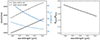 |
Fig. A.1. Resolution and line spread function (LSF) of the NIRSpec dispersers depend strongly on the light profile of the source. Left: Resolution and corresponding velocity dispersion estimated using our modelling software for a point source in the centre of the shutter and G395H grating (dashed lines). The solid lines show the dispersion curves available on the JWST user documentation webpage (JDox), which provides a (pre-launch) approximation for the LSF of a uniformly illuminated shutter. Right: Ratio of the resolution for a point source and LSF approximation for a uniform light distribution. At shorter wavelengths, the spectral resolution is higher by nearly a factor of 2 for a point source. |
Appendix B: Prism spectra and SEDs
As described in Section B, we performed SED modelling to the prism (R ∼ 100) spectroscopy of our sample using the BEAGLE software (Chevallard & Charlot 2016). We show these spectra and best-fit (minimum χ2) models in Fig. B.1.
Generally, the spectra show very blue UV continua and strong emission lines. As a result, we infer a low stellar mass and high specific SFR (median sSFR ∼ −8.0 yr−1). The stellar masses and SFRs, corrected for slit losses, are presented in Table B.1.
We also used the prism spectra to calculate the contribution of the emission lines to the NIRCam images of Fig. 1 to test our assumption that the images trace the morphology of the emission lines rather than the stellar continua. We used the sedpy software (Johnson 2019) and the observed prism spectrum to compute the total AB magnitude in the relevant NIRCam filter. Then, we constructed a spectrum with only strong emission lines (Hβ, the [OIII] doublet, Hα), using emission line fluxes measured with pPXF as described in D’Eugenio et al. (in prep.), and computed the AB magnitude in the NIRCam filter from the emission lines alone.
We present the flux ratios in Table B.2. For four out of six objects, which are observed in the medium bands, the emission lines dominate the NIRCam photometry (72% of the flux on average). For the other two objects observed in broad bands, the emission lines do not dominate, but contribute substantially to the photometry.
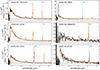 |
Fig. B.1. Prism (R ∼ 100) spectra (black lines) and best-fit SED models estimated using BEAGLE (orange lines). The emission lines used for the dynamical modelling are highlighted by dashed lines. The SEDs of all objects are very blue and show strong emission lines, pointing to young star-forming stellar populations with low stellar masses and high specific SFRs. |
BEAGLE modelling results. The values are the median of the posterior probability distributions, and the uncertainties reflect the 16th and 84th percentiles.
Ratio of the emission line fluxes to the total fluxes (continuum + emission lines) within the NIRCam filters used for the morphological modelling.
All Tables
BEAGLE modelling results. The values are the median of the posterior probability distributions, and the uncertainties reflect the 16th and 84th percentiles.
Ratio of the emission line fluxes to the total fluxes (continuum + emission lines) within the NIRCam filters used for the morphological modelling.
All Figures
|
Fig. 1. Sample of six spatially resolved high-redshift objects in JADES. The left panels show cutouts of the emission lines in the 2D rectified and combined spectra obtained with the high-resolution G395H grating. The negatives in the cutouts are the result of the background-subtraction method. The right panels show NIRCam image cutouts for each object (JADES and FRESCO) for the band that most closely resembles the emission line morphology (Sect. 2.2). The three-shutter slits and three-point nodding pattern we used result in an effective area of five shutters: The shutter encompassing the source is shown in orange, and the shutters used for background subtraction are shown in purple. |
| In the text | |
|
Fig. 2. Sample distribution in the parameter space of the stellar mass, SFR, and emission line half-light radius, colour-coded by redshift. We compare this with a selection of ground-based near-infrared spectroscopic surveys that used the Hα and [OIII] lines to measure galaxy kinematics at z ∼ 1 − 4 (Turner et al. 2017; Förster Schreiber et al. 2018; Wisnioski et al. 2019; Price et al. 2020). We used UV+IR SFRs from Whitaker et al. (2014) where available for the Turner et al. (2017) sample. We note that all objects at z > 1 from KMOS3D are shown in this figure, but not all objects were used in the kinematic studies because the S/N was low or the objects were too small. The sample selected from JADES (hexagons) probes a very different regime: JADES targets are at higher redshift and lower stellar mass than ground-based facilities have probed thus far. |
| In the text | |
|
Fig. 3. Example of the fitting procedure for object JADES-NS-00016745 (Fig. 1). Although the final combination of all exposures (left) was used for our initial visual inspection and sample selection, the pixels in this spectrum are highly correlated. Instead of using this combined spectrum, we simultaneously fit to all individual exposures obtained. In the case of JADES-NS-00016745, two exposures were taken per nodding position, resulting in six independent measurements for one three-point nodding pattern with NIRSpec. To account for the undersampled PSF of NIRSpec, we performed our modelling in the detector plane, propagating parametric models to the exact same location on the detector as the observed data. The likelihood is then computed from the combination of all residual images. Pixels flagged by the reduction pipeline as affected by cosmic rays are masked and shown in grey. |
| In the text | |
|
Fig. 4. Corner plot for the 11-parameter thin-disc model for the object in Fig. 3. Histograms show the posterior probability distributions. The orange lines indicate the prior probability distributions. We generally find good constraints on the kinematic parameters va and σ0, although the turnover radius rt is poorly constrained and degenerate with the rotational velocity. The top right panels show (in blue) the parameters that we derived from the model and are discussed in Sect. 4. |
| In the text | |
|
Fig. 5. Velocity dispersion of the ionised gas as a function of redshift. The dashed line shows the fit from Übler et al. (2019) for ionised gas at 0.6 < z < 2.6 extrapolated to higher redshifts, while the circles show results from a selection of ground-based IFU surveys in the near-infrared (Turner et al. 2017; Förster Schreiber et al. 2018) and the squares the results from ground-based near-infrared MOS data (the resolved and aligned sample of Price et al. 2020). The blue triangles show results from various studies with ALMA that measure the kinematics of the cold gas for massive, dusty star-forming galaxies (Neeleman et al. 2020; Rizzo et al. 2020; Fraternali et al. 2021; Lelli et al. 2021; Rizzo et al. 2021; Herrera-Camus et al. 2022; Parlanti et al. 2023). |
| In the text | |
|
Fig. 6. Rotational support as a function of redshift, measured as the ratio of the velocity at the effective radius and the constant velocity dispersion: v(re)/σ0. Although studies based on ground-based near-infrared data (as described in Fig. 5) have found a clear, gradual decline in v/σ toward higher redshift, we find an interesting diversity among our sample of low-mass galaxies, with dynamically cold discs existing possibly as early as z ∼ 7. |
| In the text | |
|
Fig. 7. Stellar mass versus dynamical mass (Eq. (4)) as inferred from the prism and high-resolution spectroscopy, respectively. The dashed line shows the one-to-one relation between the two masses. The data points from the literature (circles, squares) are as described in Fig. 5. As is to be expected, the dynamical masses are higher than the stellar masses for all objects in our sample. Surprisingly, however, the dynamical masses are substantially higher (up to a factor of ∼40), most likely indicating high gas masses or large systematic uncertainties in the stellar mass estimates. |
| In the text | |
|
Fig. 8. Baryonic, stellar, and gas masses (estimated using the relation between ΣSFR and Σgas from Kennicutt 1998) as fractions of the dynamical mass. We find that the gas mass, and hence the baryonic mass, is approximately one order of magnitude higher than the stellar mass. Although the inclusion of the gas component reduces the large discrepancy in mass found in Fig. 7, the difference of a factor of 3 − 4 between the dynamical and baryonic mass still remains for all but one object. |
| In the text | |
|
Fig. A.1. Resolution and line spread function (LSF) of the NIRSpec dispersers depend strongly on the light profile of the source. Left: Resolution and corresponding velocity dispersion estimated using our modelling software for a point source in the centre of the shutter and G395H grating (dashed lines). The solid lines show the dispersion curves available on the JWST user documentation webpage (JDox), which provides a (pre-launch) approximation for the LSF of a uniformly illuminated shutter. Right: Ratio of the resolution for a point source and LSF approximation for a uniform light distribution. At shorter wavelengths, the spectral resolution is higher by nearly a factor of 2 for a point source. |
| In the text | |
|
Fig. B.1. Prism (R ∼ 100) spectra (black lines) and best-fit SED models estimated using BEAGLE (orange lines). The emission lines used for the dynamical modelling are highlighted by dashed lines. The SEDs of all objects are very blue and show strong emission lines, pointing to young star-forming stellar populations with low stellar masses and high specific SFRs. |
| In the text | |
Current usage metrics show cumulative count of Article Views (full-text article views including HTML views, PDF and ePub downloads, according to the available data) and Abstracts Views on Vision4Press platform.
Data correspond to usage on the plateform after 2015. The current usage metrics is available 48-96 hours after online publication and is updated daily on week days.
Initial download of the metrics may take a while.