| Issue |
A&A
Volume 689, September 2024
|
|
|---|---|---|
| Article Number | A83 | |
| Number of page(s) | 16 | |
| Section | Catalogs and data | |
| DOI | https://doi.org/10.1051/0004-6361/202450453 | |
| Published online | 03 September 2024 | |
Chandra Survey in the AKARI deep field at the North Ecliptic Pole
Optical and near-infrared identifications of X-ray sources
1
Instituto de Astronomía, Universidad Nacional Autónoma de México Campus Ensenada,
A.P. 106,
Ensenada,
BC
22800,
Mexico
2
Instituto de Astronomía, Universidad Nacional Autónoma de México,
A.P. 70-264,
Ciudad de México,
CDMX
04510,
Mexico
3
Preuniversitario UC, Pontificia Universidad Católica de Chile,
Chile
4
Leibniz-Institut für Astrophysik Potsdam,
An der Sternwarte 16,
14482
Potsdam,
Germany
5
National Institute of Technology, Wakayama College,
77 Noshima, Nada-cho, Gobo,
Wakayama
644-0023,
Japan
6
Japan Space Forum 3-2-1, Kandasurugadai, Chiyoda-ku,
Tokyo
101-0062
Japan
7
Space Information Center, Hokkaido Information University,
Nishi-Nopporo 59-2, Ebetsu,
Hokkaido
069-8585,
Japan
8
Department of Physics, Kwansei Gakuin University,
2-1 Gakuen, Sanda,
Hyogo
669-1337,
Japan
9
University of California, Los Angeles, Division of Astronomy & Astrophysics,
430 Portola Plaza,
Los Angeles,
CA
90095-1547,
USA
10
Department of Physics and Astronomy, Seoul National University,
1 Gwanak-ro, Gwanak-gu,
Seoul
08826,
Republic of Korea
11
SNU Astronomy Research Center, Seoul National University,
1 Gwanak-ro, Gwanak-gu,
Seoul
08826,
Republic of Korea
12
Iwate University,
3-18-8 Ueda, Morioka,
Iwate
020-8550,
Japan
13
Institute of Astronomy, National Tsing Hua University,
101, Section 2, Kuang-Fu Road,
Hsinchu
30013,
Taiwan
14
Institute of Astronomy and Astrophysics, Academia Sinica,
11F of Astronomy-Mathematics Building, No. 1, Sec. 4, Roosevelt Road,
Taipei
10617,
Taiwan, ROC
15
Institute of Space and Astronautical Science, Japan Aerospace Exploration Agency, Sagamihara,
Kanagawa
229-8510,
Japan
16
The Graduate University for Advanced Studies,
SOKENDAI, Shonan Village, Hayama,
Kanagawa
240-0193,
Japan
Received:
19
April
2024
Accepted:
17
July
2024
Abstract
Aims. We present a catalog of optical and infrared (NIR) identifications (ID) of X-ray sources in the AKARI North Ecliptic Pole (NEP) deep field detected with Chandra, covering ~0.34 deg2 and with 0.5–2 keV flux limits ranging between ~2–20 × 10−16 erg s−1 cm−2.
Methods. The optical/NIR counterparts of the X-ray sources were taken from our Hyper Suprime Cam (HSC)/Subaru and Wide-Field InfraRed Camera (WIRCam)/Canada–France–Hawaii Telescope (CFHT) data because these have much more accurate source positions due to their spatial resolution than those of Chandra and longer wavelength IR data. We concentrate our identifications in the HSC g band and WIRCam Ks band-based catalogs. To select the best counterpart, we utilized a novel extension of the likelihood-ratio (LR) analysis, where we used the X-ray flux as well as g-Ks colors to calculate the likelihood ratio. The spectroscopic and photometric redshifts of the counterparts are summarized in this work. In addition, simple X-ray spectroscopy was carried out on the sources with sufficient source counts.
Results. We present the resulting catalog in an electronic form. The main ID catalog contains 403 X-ray sources and includes X-ray fluxes, luminosities, g and Ks band magnitudes, redshifts and their sources, and optical spectroscopic properties, as well as intrinsic absorption column densities and power-law indices from simple X-ray spectroscopy. The X-ray sources identified in this work include 27 Milky-Way objects, 57 type I AGNs, 131 other AGNs, and 15 galaxies. The catalog serves as a basis for further investigations of the properties of the X-ray and NIR sources in this field.
Conclusions. We present a catalog of optical (g band) and NIR (Ks band) identifications of Chandra X-ray sources in the AKARI NEP Deep field with available optical/NIR spectroscopic features and redshifts as well as the results of simple X-ray spectroscopy. In the process, we developed a novel X-ray flux-dependent likelihood-ratio analysis for selecting the most likely counterparts among candidates.
Key words: methods: data analysis / catalogs / surveys / galaxies: active / X-rays: galaxies
Corresponding author; e-mail: This email address is being protected from spambots. You need JavaScript enabled to view it.
© The Authors 2024
 Open Access article, published by EDP Sciences, under the terms of the Creative Commons Attribution License (https://creativecommons.org/licenses/by/4.0), which permits unrestricted use, distribution, and reproduction in any medium, provided the original work is properly cited.
This article is published in open access under the Subscribe to Open model. This email address is being protected from spambots. You need JavaScript enabled to view it. to support open access publication.
1 Introduction
The infrared (IR) observatory AKARI, launched in 2006 and ended its operation in 2011 (e.g., Matsuhara et al. 2005), has left an enormous legacy to the astronomical community, including two-tier dedicated surveys on the North Ecliptic Pole (NEP) region with its InfraRed Camera (IRC) (Matsuhara et al. 2006; Wada et al. 2008; Takagi et al. 2012) consisting of the AKARI NEP Deep Field (ANEPD; ~0.4 deg2) and AKARI NEP Wide Field (ANEPW; ~5.4 deg2) (Kim et al. 2012). The uniqueness of the ANEPD/W field observations lies in the complete coverage of imaging observations with the nine IRC filters, continuously covering 2–25 μm. The combination of the AKARI IRC photometric dataset, combined with other IR/optical/radio data available in this field, enables us to carry out spectral energy distribution (SED) decompositions of the sources. In particular, three filters in the 11–18 μm range have filled in a gap between Spitzer’s Infrared Array Camera (IRAC) and Multiband Imaging Photometer (MIPS) filters, giving unique mid-infrared (MIR) wavelength coverage among the deep fields that is complementary to the extensive multi-filter coverage of Mid-Infrared Instrument (MIRI). Because of the uniqueness of the AKARI data, many multi-wavelength follow-up observations have been underway. The early Subaru Suprime Cam (SCAM) data concentrated on a sub-region of ANEPD are now superseded by new Subaru Hyper Suprime Cam (HSC) data, covering the entire ANEPW data. The Galaxy Evolution Explorer (GALEX) (Burgarella et al. 2019) and Herschel (Photoconductor Array Camera and Spectrometer (PACS)/Spectral and Photometric Imaging Receiver (SPIRE) Pearson et al. 2019; Burgarella et al. 2019) observations have added ultraviolet (UV) and far infrared (FIR) coverage, respectively.
These data enabled us to carry out an IR-selection of active galactic nuclei (AGNs) by quantitatively separating the starformation and AGN torus dust emission component based on an SED decomposition (e.g., Miyaji et al. 2019; Wang et al. 2020), where the strong MIR coverage of AKARI has been key. The combination of the strong AGN component in IR and the weak X-ray (or the upper limit thereof) is a strong tool for identifying highly obscured AGNs. This is because MIR emission is not substantially affected by the absorption by intervening material, while the X-ray emission (even at E ≳ 2 keV) is heavily attenuated by Compton-thick (CT) absorbers with column densities of NH ≳ 1024cm−2. Motivated by these data, we observed the ANEPD region with our Chandra Cycle 12 (Miyaji & Akari Nep Survey Team 2020) proposal. Combined with existing data from the archive, a total of 290 ks of Chandra data have been accumulated over −0.34 deg2 and −450 X-ray sources have been detected (Krumpe et al. 2015, hereafter, K15).
While the main purpose of K15 was to present the source detection methods and a source catalog, we also identified Compton-thick AGN candidates from the IR AGN luminosity from the SED fits (Hanami et al. 2012) and the X-ray luminosity from Chandra. After the publication of K15, further follow-up observations in the ANEPD and ANEPW fields have been made, including those using Subaru HSC (optical) (Oi et al. 2021; Kim et al. 2021), Herschel (FIR, Pearson et al. 2019; Burgarella et al. 2019), GALEX (UV Burgarella et al. 2019). Furthermore, submillimeter (submm) and radio observations have also been carried out with observatories, including the Westerbork Synthesis Radio Telescope (WSRT, White et al. 2010) and the Karl G. Jansky Very Large Array (JVLA, Ishigaki et al. in prep.).
Even with the very high spatial resolution (≲1″) of Chandra near its optical axis, the point spread function (PSF) degrades rapidly with off-axis angle, from sub-arcsecond on-axis to ~5 arcsec (50% energy-encircled radius) at the off-axis angle of 10 arcmin1. Usually for survey observations, including ANEPD, data from the entire field of view (FOV) of the four ACIS-I CCDs (−16′ × 16′) are used. The Chandra observations of ANEPD are arranged such that the FOVs of 12 (our program) + 2 (archive) observations overlap with neighboring ones. Thus, a particular point in the sky could be observed with multiple off-axis angles with different PSFs. Our source detection algorithms described in K15 take full advantage of the overlapped observations by a simultaneous PSF fitting over overlapped fields. These utilize the Chandra version of emldetect of the XMM-Newton SAS package, simultaneously making multiple PSF fits over the observations with different off-axis angles and energy bands. The positional uncertainty of the source reflects the distribution of the off-axis angles over observations and net counts for each contributing observation. In this method, if there are sufficient photon counts in the observations with small off-axis angles, we get good source positions, even if other observations are at large off-axis angles. However, the sum of photons of all observations contributes to good spectral analysis. However, near the edges of the Chandra ANEPD, which are only covered at large off-axis angles, the positional uncertainties can be as large as a few arcseconds. Therefore, there are still X-ray sources with multiple counterpart candidates. There are several methods to select the most likely counterpart(s) of a source at a certain wavelength with higher positional uncertainty in catalogs with much lower positional uncertainty. One such method is the likelihood ratio (LR) technique developed by Sutherland & Saunders (1992), which is frequently used in X-ray surveys (e.g., Brusa et al. 2007; Civano et al. 2012; Marchesi et al. 2016). One of the factors of LR is the optical magnitude distribution of X-ray sources q(m). Salvato et al. (2018) extended the LR to include multi-band photometry and introduced q(m), which is a function of magnitudes from multi-band photometry. While q(m) or q(m) can be highly X-ray flux dependent, these authors used a single q(m) or q(m) for the entire X-ray source population in the respective surveys (or larger surveys at a similar depth). Salvato et al. (2018, 2022) used a public code for a general Bayesian-based identification algorithm, NWAY, developed by J. Buchner. While the code allows for very flexible prior specifications, the X-ray flux dependence of q(m) has not been included in their prior. In this paper, we present a catalog of Chandra X-ray source identifications in the AKARI NEP deep field presented in K15. Due to the positional accuracy, we primarily found X-ray counterparts in the Gaia, Subaru HSC-g and Canada–France–Hawaii Telescope (CFHT) Wide-Field InfraRed Camera (WIRCam) Ks band catalogs. In selecting the most likely counterpart, we developed the novel X-ray flux-dependent two-band LR technique. In Sect. 2, we explain the source of X-ray, optical-IR imaging, and optical/IR spectroscopy data as well as the sample used in our analysis. In Sec. 3, we explain our identification procedure, including the X-ray flux-dependent two-band likelihood ratio technique. In Sec. 4, we present our results including the explanation of our identification catalog, while the catalog itself is published in an electronic version only. In Sec. 5, we discuss the results of the identification process. We summarize our work in Sec. 6. In Appendix A, we present the results from our series of multi-object spectroscopic observations using the Gran Telescopio Canarias (GTC)/Optical System for Imaging and low-Resolution Integrated Spectroscopy (OSIRIS) and the Large Binocular Telescope (LBT)/Multi-Object Double Spectrograph (MODS). These observations are mainly targeted on the AGNs in ANEPD, including (but not limited to) the Chandra sources presented in Sec. 2. For luminosity calculations, we used a Λ-CDM cosmology with H0 = 70h70 km s−1 Mpc−1, Ωm = 0.3, and ΩΛ = 0.7.
2 Observation and data
2.1 Chandra observations
The details of the Chandra observations are explained and the point source catalog of the ANEPD is presented in K15. Here, we briefly summarize the basic aspects.
The field was observed with Chandra between December 2010 and April 2011 (cycle 12). Twelve individual ACIS-I pointings with a total exposure time of 250 ks were awarded. The OBSIDs are 12925, 12926, 12927, 12928, 12929, 12930, 12931, 12932, 12933, 12934, 12935, 12936, and 13244. The central position of the mosaicked observation is roughly RA = 17h 55m 24s and Dec = +66° 33′ 33″. In addition, we include two Chandra ACIS-I pointings from the archive (10443, 11999), which have observed the southeast corner of the AKARI NEP deep field. The total area covered by our Chandra mosaicked survey is ~0.34 deg2. This almost completely covers early deep optical and near-infrared (NIR) images covering 26.3 arcmin × 33.7 arcmin (~0.25 deg2) with earlier Subaru/SCAM and KPNO/Flamingos respectively. The observation has been designed to reach an approximately homogeneous coverage of typically ~30–40 ks. In the region with the additional pointings from the archive (OBSIDs 10443 and 11999), we were able to reach a depth of ~80 ks. In K15, we made an astrometric correction for each OBSID by cross-matching X-ray source positions with trivial counterparts in the Subaru/SCAM images. A total of 457 sources are listed in the main source catalog of K15, with flux limits corresponding to 50% of the survey area are 3 × 10⁻¹⁵, 8 × 10⁻¹⁶, and 4 × 10⁻¹⁵ (erg s−1 cm−2) for the 0.5–7, 0.5–2, and 2–7 keV bands, respectively. The flux limits on the deepest area are 1 × 10⁻¹⁵, 2 × 10⁻¹⁶, and 1 × 10⁻¹⁵ (erg s−1 cm−2) for the respective bands.
2.2 Gaia, Subaru/HSC and CFHT/WIRCam data
In this paper, we find counterparts from optical and IR data with a higher resolution and positional accuracy than the X-ray data. For this purpose, we used Gaia Data Release 3 (DR3)2 as well as our HSC/Subaru and our WIRCam/CFHT data (Oi et al. 2014; Kim et al. 2021; Oi et al. 2021).
For the HSC data, we used our internal band-merged catalog, which has been produced as a part of the work by Kim et al. (2021); whereas those with AKARI counterparts were made public along with the paper3, however, the internal catalog includes HSC sources that are not AKARI sources. This catalog is slightly updated from the one by Oi et al. (2021). Among those HSC band-merged sources, we selected those that are detected in the g-band at more than 4σ and within our Chandra FOV. We chose the g-band, because there are the largest number of >4σ detections among the five HSC bands. The positions of the sources in the band-merged HSC catalogs are forced to be the same in the five grizy bands, making it easy to find photometries in other bands. Our WIRCam/CFHT KS band-based catalog was produced as a part of the work by (Oi et al. 2014), which also selected by 4σ detections in this band.
Figure 1 shows g and Ks band magnitude distributions (N(m)/dm) within our Chandra FOV. For comparison, the N(m) distributions for the COSMOS field are overplotted for the HSC g-band from the HSC-Subaru Strategic Program Data Release 2 (SSP-2) (Aihara et al. 2019)4 and WIRCam/CFHT Ks(Laigle et al. 2016). The g band magnitudes have been corrected for the Galactic extinction.
The COSMOS data are used as a template for the likelihood ratio analysis described below. We see that the HSC-g band data have similar depths in both fields, while COSMOS has much deeper WIRCam Ks data. The HSC g-band counts drop suddenly at g ≲ 20 due to image saturations. The Gaia catalog, which shows that the g-band magnitudes nicely complement the HSC-g data at the bright end.
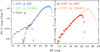 |
Fig. 1 Number counts inin ANEPD. (a) Number counts dN(n)/dm (deg−2 mag−1) of g-band sources in the AKARI NEP Deep Field (within the Chandra field, from Gaia and HSC) and the COSMOS field (HSC). (b) Number counts for the Ks band. Both come from CFHT/WIRCam. |
2.3 Optical and IR spectroscopy
Many of the X-ray source candidates have spectroscopic observations in the optical-IR bands from various programs, some are from AKARI NEP survey team, others from the archive. The source of spectroscopic data includes Hectspec/Multiple Mirror Telescope (MMT), Hydra/WIYN (Shim et al. 2013), Deep Imaging Multi-Object Spectrograph (DEIMOS)/Keck from our 2008 and 2011 runs, (Churei 2013; Shogaki 2018; Kim et al. 2021), FMOS/Subaru (Oi et al. 2017), OSIRIS/Gran Telescopio Canarias (GTC, Appendix A), the SPICY program using the non-slit spectroscopy mode of AKARI InfraRed Camera (IRC) (Ohyama et al. 2018). The results of our newer observations with DEIMOS and Multi-Object Spectrograph for Infrared Exploration (MOSFIRE/Keck starting 2014 (Kim et al. 2020), Hectspec/MMT observed in 2020–2022 (Kim et al. 2024), and the large binocular telescope (LBT, Appendix A) are also included.
3 Identification procedure
3.1 Selecting counterpart candidates
The X-ray source positions in K15 have been calibrated based on the SCAM data, which are offset from astrometric solutions of our HSC and CFHT WIRCam data. Before attempting the cross-identification with the HSC and WIRCam sources, we adjusted the X-ray source positions by δThisPaper = δK15 + 0.3″, where δ represents the declination, to match the astrometry of the HSC/WIRCam data. The systematic offset of the RA direction between SCAM and HSC/WIRCam data as well as those among Gaia, HSC, and WIRCam data are negligible for our purposes (<0.1″).
In K15, we have derived an empirical total positional uncertainty of ![Mathematical equation: $\[\sigma_{\text {total }}=5 \times \sqrt{\sigma_{\text {sys. }}^2+\sigma_{\text {stat. }}^2}\]$](/articles/aa/full_html/2024/09/aa50453-24/aa50453-24-eq1.png) , where σstat is the statistical positional uncertainties of our maximum-likelihood fitting, while σsys = 0.1 arcsec is the systematic error. Further considering the astrometric uncertainties of σastro = 0.2 arcsec, we defined the matching radius of
, where σstat is the statistical positional uncertainties of our maximum-likelihood fitting, while σsys = 0.1 arcsec is the systematic error. Further considering the astrometric uncertainties of σastro = 0.2 arcsec, we defined the matching radius of ![Mathematical equation: $\[r_{\text {match }}=\sqrt{\sigma_{\text {total }}^2+\sigma_{\text {astro }}^2}\]$](/articles/aa/full_html/2024/09/aa50453-24/aa50453-24-eq2.png) . We note that the notations σtotal and σastro, introduced in K15, do not represent the standard deviations of any Gaussian. These roughly correspond to 5σ in the typical sense.
. We note that the notations σtotal and σastro, introduced in K15, do not represent the standard deviations of any Gaussian. These roughly correspond to 5σ in the typical sense.
We looked for optical counterparts in the Gaia DR3, HSC/Subaru-g band, and WIRCam/CFHT-Ks band selected sources within rmatch. For finding genuine X-ray source counterparts, we used our novel X-ray flux-dependent two-band likelihood ratio analysis, after excluding special cases. These special cases include those X-ray sources that are part of an extended source and cataloged spuriously as multiple point sources in K15, those sources that are close to the very edge of the combined Chandra FOV, and the bright sources that are detected in Gaia DR3 (a majority of which are saturated in our HSC g band data). We list the X-ray sources in the category of these special cases in Sec. 4.
3.2 X-ray flux-dependent two-band likelihood ratio analysis
3.2.1 Formalism
A common procedure for selecting counterparts among multiple candidates is the likelihood ratio (LR) technique, which has been extensively used for finding X-ray source counterparts (e.g., Brusa et al. 2007; Civano et al. 2012; Marchesi et al. 2016). It was originally developed by Sutherland & Saunders (1992) for the identification of radio sources. The conventional likelihood ratio LRconv is defined by
![Mathematical equation: $\[\begin{aligned}L R_{\mathrm{conv}} & =\frac{q(m) f(r)}{n(m)}, \\\int_{-\infty}^{\infty} q(m) d m & =1, \quad \int_0^{\infty} 2 \pi r~ f(r)~ d r=1,\end{aligned}\]$](/articles/aa/full_html/2024/09/aa50453-24/aa50453-24-eq3.png) (1)
(1)
where q(m) is the apparent magnitude distribution (per mag) of the genuine X-ray source counterparts, f(r) is the probability density (per solid angle) that the source is at the angle r away from the cataloged X-ray source position, and n(m) is the number density (per solid angle per mag) of the optical sources as a function of apparent magnitude. The (non-conventional) likelihood ratio (LR) has no units. In practice, q′ = qQ and LR′ = LR Q, where Q is the fraction of the genuine X-ray source counterparts that are within the optical or IR sample (see Sec. 3.3 for our method for estimating Q).
Traditionally, for simplicity, q(m) is assumed universal over X-ray sources, independent of their X-ray properties, including the flux. Since the flux of our X-ray sources ranges over four orders of magnitude, we go one step further and consider a flux-dependent likelihood ratio. Furthermore, we analyze two bands of the counterpart candidates simultaneously (HSC-g and WIRCam Ks bands). Including these aspects, we use in this work the following expression for the likelihood ratio:
![Mathematical equation: $\[L R^{\prime}=\frac{q^{\prime}\left(g, K_{\mathrm{s}} {\mid} S_{\mathrm{X}}\right) f(r)}{n\left(g, K_{\mathrm{s}}\right)}, ~\iint q^{\prime}\left(g, K_{\mathrm{S}}\right) d g ~d K_{\mathrm{s}}=1,\]$](/articles/aa/full_html/2024/09/aa50453-24/aa50453-24-eq4.png) (2)
(2)
where q′(g, Ks|SX) is the two-dimensional (2D) g-Ks magnitude distribution of the X-ray source counterparts given an X-ray flux SX. For the normalization of q′, the integration limits are defined by the sample.
For those sources with both g-band and Ks band detections within the magnitude limits of the sample, we assume that q′(g, Ks|SX) is a product of two Gaussians, one in A = log SX + 0.4g (logarithm of the X-ray to optical flux ratio) and the other in B = g − Ks, with their mean values of Ā and ![Mathematical equation: $\[\bar{B}\]$](/articles/aa/full_html/2024/09/aa50453-24/aa50453-24-eq5.png) and the standard deviations σA and σB, respectively. The parameters Ā,
and the standard deviations σA and σB, respectively. The parameters Ā, ![Mathematical equation: $\[\bar{B}\]$](/articles/aa/full_html/2024/09/aa50453-24/aa50453-24-eq6.png) , σA, and σB can depend on SX. Thus, it is expressed as:
, σA, and σB can depend on SX. Thus, it is expressed as:
![Mathematical equation: $\[\begin{aligned}q^{\prime}\left(g, K_{\mathrm{S}} {\mid} S_{\mathrm{X}}\right) \propto & \exp \left[-\frac{(A-\bar{A})^2}{2 \sigma_{\mathrm{A}}^2}\right] \exp \left[-\frac{(B-\bar{B})^2}{2 \sigma_{\mathrm{B}}^2}\right] \\& \left(A_{\min } \leq g \leq A_{\max }, B_{\min }<B<B_{\max }\right) \\& =0, \text { (otherwise) }.\end{aligned}\]$](/articles/aa/full_html/2024/09/aa50453-24/aa50453-24-eq7.png) (3)
(3)
The Gaussian components of Eq. (3) are truncated at respective A and B values corresponding to the minimum and maximum g and g − Ks magnitudes in the template sample (see below):
![Mathematical equation: $\[A_{\min }=\log S_{\mathrm{X}}+0.4 ~g_{\min }, \quad A_{\max }=\log S_{\mathrm{X}}+0.4 ~g_{\max },\]$](/articles/aa/full_html/2024/09/aa50453-24/aa50453-24-eq8.png) (4)
(4)
![Mathematical equation: $\[B_{\min }=\left(g-K_{\mathrm{s}}\right)_{\min }, \quad B_{\max }=\left(g-K_{\mathrm{s}}\right)_{\max },\]$](/articles/aa/full_html/2024/09/aa50453-24/aa50453-24-eq9.png) (5)
(5)
We note the truncation limits of A depend on SX. We assume that the center and standard deviation of the Gaussian factor, for instance, for the variable A follow the power-law form of SX:
![Mathematical equation: $\[\sigma_{\mathrm{A}}=\sigma_{\mathrm{A}, 14} ~S_{\mathrm{X}, 14}^{\alpha_{\mathrm{A}}}, \quad \bar{A}=\bar{A}_{14} ~S_{\mathrm{X}, 14}^{\beta_{\mathrm{A}}},\]$](/articles/aa/full_html/2024/09/aa50453-24/aa50453-24-eq10.png) (6)
(6)
where SX,14 is SX (0.5–7 keV) measured in the units of 10−14 erg s−1 cm2. We use the forms of SX dependence for B by replacing A in Eq. (6) by B.
The motivation of the first Gaussian is the observation that the distribution of X-ray sources in the X-ray flux-optical flux plane is concentrated along a constant SX/Fopt line (e.g., Fig. 11 of Marchesi et al. 2016) with spread around it. In reality, the distribution perpendicular to the line is asymmetric and there is a wing toward the lower SX/Fopt end, representing host galaxy dominant AGNs and stars. However, if we include proper g magnitude limits in the HSC data, the Gaussian form still gives a good approximation, as shown below. As another factor in the distribution, a Gaussian in B(= g − KS) is assumed, attempting to be as independent as possible with the A distribution. A possible correlation between A and B is neglected, which is reasonable for our purpose.
In cases where the candidate is detected in the g-band, but not in the Ks band (and vice versa), we apply the following expressions for Ag = log SX + 0.4g and AK = log SX + 0.4Ks:
![Mathematical equation: $\[\begin{aligned}q^{\prime}\left(A_g {\mid} S_{\mathrm{X}},!K_{\mathrm{s}}\right) & \propto \exp \left[-\frac{\left(A_g-\bar{A_g}\right)^2}{2 \sigma_{\mathrm{A}_g}^2}\right], \\q^{\prime}\left(A_K {\mid} S_{\mathrm{X}},!g\right) & \propto \exp \left[-\frac{\left(A_K-\bar{A_K}\right)^2}{2 \sigma_{\mathrm{A}_{\mathrm{K}}}^2}\right].\end{aligned}\]$](/articles/aa/full_html/2024/09/aa50453-24/aa50453-24-eq11.png) (7)
(7)
Here, !Ks and !g mean non-detection in Ks and g, respectively. We use the forms of SX dependence for Ag (AK) by replacing A in Eq. (6) by Ag (AK). The denominator of LR′ (cf. Eq. (2)) should now be n(g, !Ks), which is the number density per g-magnitude of galaxies that are not detected in Ks, or n(Ks, !g) defined likewise. For Eqs. (3) and (7), the normalization of q′ is determined such that the integral over the magnitudes, considering appropriate magnitude limits, becomes unity when SX is given.
3.2.2 Estimating q′-functions using the COSMOS Legacy template
The q(m) function in Eq. (1) is often estimated by subtracting the magnitude distribution of optical sources around a certain radius (~ positional errors) around X-ray sources by that of the field scaled by the relative solid angles of the source area and the field. However, in our work, this method is subject to shot noise at certain regimes, by including X-ray flux dependence and treating two-band optical identifications. Another method is to use an identification catalog of another survey that includes sources with a similar X-ray flux range as our data as a template. Such a survey should have reliable counterparts. For this purpose, we use the source identification catalog of the COSMOS Legacy survey by Marchesi et al. (2016). While they used LRconv, the COSMOS Legacy survey has deeper exposures, larger survey area, and highly overlapping ACIS-I exposures covering a total of ~2.2 deg2 within which ~1.7 deg2 are uniformly covered at ~160ks of exposure (Civano et al. 2016). The highly overlapping configuration makes the most of the survey area observed with, on average, smaller off-axis angles. In the COSMOS field, an extensive optical-IR dataset, including the HSC-g band (Tanaka et al. 2017; Aihara et al. 2019) and Ks band from CFHT (and Ultra-Vista) exist, which makes this data convenient for our template. Typically, the offsets between COSMOS Legacy X-ray sources and the counterparts above their LR-threshold are ~0.7′. In constructing our q′(g, KS) function, we used the i and Ks counterparts of COSMOS Legacy X-ray sources from Marchesi et al. (2016), with the new g-band photometry by HSC SSP-2 (Sec. 2.2) at the positions of the i-band counterpart. We considered an HSC source that is within 0.7″ of the original i-band position to be of the same source. The choice of this separation is that this corresponds to the minimum separation, with very few exceptions, between two different sources in the HSC catalog. We note that, due to the saturation of the HSC data, the brightest sources in the g-band (g ≤ 19.5) are not included.
As shown in Fig. 1, the depths of the HSC g-band data are similar between the COSMOS Legacy and ANEPD fields, while the WIRCam Ks data are ~2 mag deeper in the COSMOS deep field. Thus, for the template q′-function, we randomly removed fainter Ks detections of the COSMOS Legacy identifications refer to instances where the number counts agree with those of the ANEPD field. Based on the number counts in Fig. 1, we find that the ratio of the ANEPD and COSMOS number counts can be represented by 1 − 0.1025(Ks − 20.3)2.3 at Ks > 20.3. Therefore, for a COSMOS Legacy ID with Ks > 20.3, a random number R (0 ≤ R ≤ 1) is generated and if R < 1 − 0.1025(Ks − 20.3)2.3, we treated this source as undetected in Ks for our template purposes. We excluded those bright sources that are saturated in the HSC image for the template catalog. For the X-ray candidates that are saturated in the HSC image in our ANEPD field, we used the Gaia DR3 catalog and treated them separately.
The parameters of the Eqs. (3) and (7) is determined by a maximum likelihood fitting of the function over the template ID catalog. The expected number density of objects in the template sample can be expressed by:
![Mathematical equation: $\[F\left(g, K_{\mathrm{s}}, S_{\mathrm{X}}\right)=d N\left(S_{\mathrm{X}}\right) / d \log \left(S_{\mathrm{X}}\right) \cdot q\left(g, K_{\mathrm{s}} {\mid} S_{\mathrm{X}}\right),\]$](/articles/aa/full_html/2024/09/aa50453-24/aa50453-24-eq12.png) (8)
(8)
where dN/d log SX is the number of X-ray sources per log SX as a function of X-ray flux and is approximated by a smoothed two power-law form with a shoulder flux at SX = SX,b:
![Mathematical equation: $\[d N / d \log S_{\mathrm{X}} \propto\left[\left(S_{\mathrm{X}} / S_{\mathrm{X}, \mathrm{b}}\right)^{-\gamma_1}+\left(S_{\mathrm{X}} / S_{\mathrm{X}, \mathrm{b}}\right)^{-\gamma_2}\right]^{-1},\]$](/articles/aa/full_html/2024/09/aa50453-24/aa50453-24-eq13.png) (9)
(9)
where dN/d log SX ∝ γ1 and dN/d log SX ∝ γ2 asymptotically at the faint and bright ends, respectively.
In our maximum-likelihood method, (e.g., Miyaji et al. 2015), we first found the best-fit parameter values of the X-ray number counts Eq. (9), namely, α1, α2, and log SX,b by minimizing:
![Mathematical equation: $\[\mathcal{L}_{\mathrm{NS}}=-2 \sum_i \frac{d N / d \log S_{\mathrm{X}, \mathrm{i}}}{\int\left(d N / d \log S_{\mathrm{X}}\right) d \log S_{\mathrm{X}}},\]$](/articles/aa/full_html/2024/09/aa50453-24/aa50453-24-eq14.png) (10)
(10)
where i is over the objects in the template catalog that have both g and Ks detections. Then, the parameters in Eq. (6) can be determined by minimizing
![Mathematical equation: $\[\mathcal{L}_{\mathrm{q}}=-2 \sum_i \frac{\left(d N / d \log S_{\mathrm{X}, \mathrm{i}}\right) q\left(g, K_{\mathrm{s}} {\mid} S_{\mathrm{X}}\right)}{\iiint\left(d N / d \log S_{\mathrm{X}, \mathrm{i}}\right) q\left(g, K_{\mathrm{s}} {\mid} S_{\mathrm{X}}\right) d K_{\mathrm{S}} ~d g ~d \log S_{\mathrm{X}}},\]$](/articles/aa/full_html/2024/09/aa50453-24/aa50453-24-eq15.png) (11)
(11)
where the parameters of (dN/d log SX,i) are now fixed. The best-fit parameters and the minima and maxima of the relevant magnitudes (Eq. (5)) are summarized in Table 1. The distribution of the objects in the template catalog is compared with those calculated from the model in Fig. 2 for the X-ray flux, A = log SX + 0.4g, and B = g − Ks. For the latter two, comparisons are made in low and high X-ray flux regimes as indicated in the figure labels, where the division is about the median of the template sample.
The basic steps are the same as those outlined above for the case of HSC g (Ks) band-only detection in the template sample. Instead of Eq. (3), Eq. (7) can be used. The best-fit parameters for these one-band detection cases are also shown in Table 1. The comparisons of the distributions in the template sample for the one-band detection cases are shown in Figs. 3 and 4.
Best-fit parameters for q′(g, Ks|SX), q′(g|!Ks, SX), and q′(Ks|!g, SX).
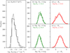 |
Fig. 2 Histograms for sources detected in both g and Ks bands for template sample with models. (a) Histogram showing the dN/d log SX distribution of the template sample of X-ray sources that have both g and Ks, constructed from the COSMOS Legacy survey. The curve shows the best-fit model. (b, c) Histograms of log SX + 0.4g distribution of the template sample and the best-fit model (curve) for the high and low flux regimes respectively as labeled. (d, e) Same as (b, c) for the g − Ks distributions. In all panels, SX is the 0.5–7 keV flux in units of erg s−1 cm−2. |
3.2.3 Estimating LR′ for the AKARI NEP X-ray Source Candidates
An important factor in LR′ is the probability that the X-ray source is at the counterpart’s candidate position, and it is normally assumed to be a function of the distance (r) between the best-fit X-ray position and that of the counterpart candidate, expressed by f(r). The source catalog published as a part of K15 has a column RADEC_ERR, which is the statistical 1σ error (σstat.) of the fitted position projected to an axis. The function f(r) can be expressed by a 2D Gaussian with a standard deviation of ![Mathematical equation: $\[\sigma_{\mathrm{pos}}=\sqrt{\sigma_{\text {stat. }}^2+\sigma_{\text {sys. }}^2}\]$](/articles/aa/full_html/2024/09/aa50453-24/aa50453-24-eq17.png) with σsys = 0.1″, namely,
with σsys = 0.1″, namely, ![Mathematical equation: $\[f(r)=\exp \left[-r^2 /\left(2 \sigma_{\text {pos }}^2\right)\right] /\left(2 \pi \sigma_{\text {pos }}^2\right)\]$](/articles/aa/full_html/2024/09/aa50453-24/aa50453-24-eq18.png) . The astrometric accuracy σastro = 0.2″ is negligible. Figure 8 of K15 shows the comparison of the distribution of the positional deviation between simulated sources and the corresponding detected source positions from the simulated image and that from the assumed f(r), which agree well with each other. For our X-ray source counterpart search, we apply the LR analysis to the HSC-g and WIRCam Ks sources within the matching radius, rmatch.
. The astrometric accuracy σastro = 0.2″ is negligible. Figure 8 of K15 shows the comparison of the distribution of the positional deviation between simulated sources and the corresponding detected source positions from the simulated image and that from the assumed f(r), which agree well with each other. For our X-ray source counterpart search, we apply the LR analysis to the HSC-g and WIRCam Ks sources within the matching radius, rmatch.
The denominator of LR′ (Eq. (2)) represents the background density distribution of optical/IR sources as a function of g and Ks magnitudes and is proportional to the probability that the X-ray source candidate is a chance coincidence. We construct edq′(g, Ks|SX), q′(g|!Ks,SX), and q′(Ks|!g, SX) from the template sample from the COSMOS Legacy Survey above. On the other hand, we constructed n(g, Ks) from our AKARI NEP dataset. To construct n(g, Ks) (both g and Ks detections), we built a 2D histogram (in steps of 1 mag. for both bands) of the number density (per unit solid angle) of the combined HSC-g and WIRCam Ks sources per solid angle within the Chandra FOV and estimated the value by a 2D cubic spline fit. For n(g|!Ks), we spline-interpolated a 1D histogram in g (in steps of 1 mag,) for the HSC g-band detected sources without a WIRCam Ks band detection. Similarly for n(Ks|!g), we spline-interpolated a 1D histogram in Ks (in steps of 1 mag) for the WIRCam Ks-band detected sources without an HSC g band detection.
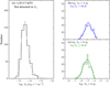 |
Fig. 3 Histograms for sources detected in g, but not detected in Ks for template sample with models. (a) Histogram showing the dN/d log SX distribution of the template sample of X-ray sources that are detected in HSC g-band, but not in CFHT Ks (depth matched with AKARI NEP Deep Field; See text), constructed from the COSMOS Legacy survey. The curve shows the best-fit model. (b, c) Histograms of log SX + 0.4 g distribution of the template sample and the best-fit model. |
3.3 Threshold determination
Once we have the LR′ value for each candidate (or LR = LR′Q), we can select the most likely counterpart from those candidates that have LR > LRth, where LRth is the threshold. Some authors take the maximum of (R + C)/2 as the threshold (e.g., Marchesi et al. 2016), while others (e.g. Brusa et al. 2007; Civano et al. 2012; Salvato et al. 2022) use R = C. In this work, we use R = C to determine LRth. Before defining R for the whole sample, we define Rj as the reliability of the j-th optical/IR object that is a candidate counterpart of any X-ray source. This is computed by
![Mathematical equation: $\[R_j=\frac{(L R)_j}{\sum_i(L R)_i+(1-Q)}=\frac{(L R)_j^{\prime} Q}{\sum_i(L R)_i^{\prime} Q+(1-Q)},\]$](/articles/aa/full_html/2024/09/aa50453-24/aa50453-24-eq19.png) (12)
(12)
where Q is the fraction of genuine X-ray source counterparts that are in the optical catalog introduced in Sect. 3.2.1. The sum is over all the candidates (indexed by i) that are the counterpart candidates of the same of the X-ray source. For the sake of simplicity, we explain the case of the conventional single-band optical catalog with a magnitude limit mlim here. In this case, Q can be expressed by
![Mathematical equation: $\[Q=\frac{\int_{-\infty}^{m_{\lim }} q(m) ~d m}{\int_{-\infty}^{\infty} q(m) d m}.\]$](/articles/aa/full_html/2024/09/aa50453-24/aa50453-24-eq20.png) (13)
(13)
If the sample has a “soft” flux limit, the numerator can be expressed by ∫ q(m)p(m)dm, where p(m) is the probability that an object with a magnitude, m, is in the optical sample.
To calculate Q based on Eq. (13), we need to integrate q(m) to m = ∞. The exact form of q(m) fainter than the magnitude limit is unknown, but it does not have any significance. However, its integration is important. The Q value can be estimated by the fraction of X-ray sources that have no candidate (fnocand) using the following relation:
![Mathematical equation: $\[N_{\mathrm{X}} Q=N_{\mathrm{X}}\left(1-f_{\text {nocand }}\right)-\sum_k\left(1-\sum_i R_i\right)_k,\]$](/articles/aa/full_html/2024/09/aa50453-24/aa50453-24-eq21.png) (14)
(14)
where k is over the X-ray sources that have at least one candidate and i is over the candidates for each X-ray source, j is over the candidates of the k-th source. The first part on the right-hand side (R.H.S.) is the number of sources that have at least one candidate. The second part (the sum over k) represents the number of sources with candidates, where the genuine candidate is not among them. This can be understood by observing that Ri is the probability of the i-th candidate being genuine. We note that ∑iRi itself contains Q (Eq. (12)). We can estimate Q based on the fraction of X-ray sources that have no candidate and LR of each candidate. We went on to consider the X-ray flux dependence exhibited by Q, which is described in Sec. 4.2.
The reliability over the whole sample is defined by R = NID/NLR>LRth, where NID is the number of identifications above the threshold, namely, the sum of all the Ri values of the candidate with LR > LRth over all the X-ray sources. Then, ![Mathematical equation: $\[N_{L R>L R_{\mathrm{th}}}\]$](/articles/aa/full_html/2024/09/aa50453-24/aa50453-24-eq22.png) is the number of all candidates above the threshold. The completeness is defined by C = NID/NX where NX is the number of X-ray sources, both are functions of LR. Once we have R and C, we can choose our threshold as the LR value at R = C.
is the number of all candidates above the threshold. The completeness is defined by C = NID/NX where NX is the number of X-ray sources, both are functions of LR. Once we have R and C, we can choose our threshold as the LR value at R = C.
4 Analysis and results
4.1 X-ray sources precluded from the LR analysis
Before attempting the LR analysis, we identified the cataloged X-ray sources (K15 primary catalog) that were not appropriate for assessing LR (Eq. (2)) values for their candidate counterparts. As a result, we precluded these sources from being included in the LR analysis.
The X-ray sources at the very edge of the combined Chandra FOV were excluded. These are sources with a candidate search area (i.e., a circular region with a radius rmatch from the X-ray nominal position, as described in Sec. 3.1) that goes beyond the edge of the FOV. These are: ANEPD-CXO392, ANEPD-CXO372, and ANEPD-CXO391.
The source detection algorithm of K15 has recognized extended emission from clusters of galaxies as multiple point-like X-ray sources. Extended emission from two clusters are recognized in our Chandra data (Huang et al. 2021), one of which is previously known as RXJ1757.3+6631 and the other is near our Chandra FOV at (α, δ) =(17:55:12,+66:33:51). The former is cataloged as ANEPD-CXO382, ANEPD-CXO436, ANEPD-CXO370, and ANEPD-CXO311. The latter is cataloged as: ANEPD-CXO297, ANEPD-CXO257, ANEPD-CXO456, ANEPD-CXO417, ANEPD-CXO208, and ANEPD-CXO302. We did not consider these as true point-like sources but as parts of extended X-ray emission and therefore they were excluded.
Díaz Tello et al. (2017) found that ANEPD-CXO104 is an ultraluminous X-ray source (ULX) in one of the spiral arms of a nearby galaxy (z =0.027). ANEPD-CXO434 is located at the center of this galaxy. These are also excluded from the LR analysis.
Bright sources with g ≤ 19.5 are mostly saturated in the HSC-g data and they are mostly absent in the HSC catalog. There are a few sources with gHSC < 19.5 (HSC). However, they are also saturated in the image near the center, and their magnitudes are not reliable. All of them are, in the Gaia DR3 catalog. Due to the very low probability of chance coincidence, we considered the Gaia sources without HSC-g counterpart or gHSC < 19.5 as secure candidates without calculating LR, but we did assign a large value (9.99 × 1029) in the main identification table.
4.2 LRth for the sample
We determined the LR threshold following the procedure described in Sec. 3.3. As a preparation, we determined the X-ray flux-dependent fnocand value to estimate Q(SX). Figure 5a shows the fraction of our ANEPD X-ray sources that have no candidate as a function of X-ray flux (Nnocand/NX). The approximate 1σ errors roughly estimated by ![Mathematical equation: $\[\sqrt{N_{\text {nocand }}} / N_{\mathrm{X}}\]$](/articles/aa/full_html/2024/09/aa50453-24/aa50453-24-eq23.png) are also plotted. We see that there is no such X-ray source at SX ≥ 1 × 10⁻¹⁴ (erg cm−2 s−1), while fnocand values are consistent with the average value of 0.11 for all the fainter bins. Using Eqs. (14) and (12), where NX = 299 is the number of X-ray sources at SX < 1 × 10⁻¹⁴ (erg cm−2 s−1) in our sample, we found Q = 0.67. Thus, we used Q = 1 for SX ≥ 1 × 10⁻¹⁴ (erg cm−2 s−1) and Q = 0.67 for SX < 1 × 10⁻¹⁴ (erg cm−2 s−1), respectively.
are also plotted. We see that there is no such X-ray source at SX ≥ 1 × 10⁻¹⁴ (erg cm−2 s−1), while fnocand values are consistent with the average value of 0.11 for all the fainter bins. Using Eqs. (14) and (12), where NX = 299 is the number of X-ray sources at SX < 1 × 10⁻¹⁴ (erg cm−2 s−1) in our sample, we found Q = 0.67. Thus, we used Q = 1 for SX ≥ 1 × 10⁻¹⁴ (erg cm−2 s−1) and Q = 0.67 for SX < 1 × 10⁻¹⁴ (erg cm−2 s−1), respectively.
Figure 5b shows the reliability (R), completeness (C), and (R + C)/2 (Sec. 3.3) as a function of the likelihood ratio threshold (LRth). As seen in this figure, R increases, and C decreases with Lth. Our (R + C) curve is rather flat with no strong peak. Thus, in our dataset, it is more beneficial to take the threshold at R = C, which is at log LRth = −2.8.
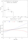 |
Fig. 5 Unidentified source fraction and reliability-completeness analysis. (a) Fraction of X-ray sources that have no candidate in any of our HSC-g, Gaia-g or WIRCam-Ks catalog as a function of SX with the histogram binsize of dex in flux. Approximate 1σ errors are also shown. (b) Reliability (R), completeness (C) and (R + C)/2 curves as a function of log LRth, as labeled. |
4.3 X-ray spectral analysis
As part of the main catalog, we list the results of a simple X-ray spectral analysis for the sources that have net 0.5–7 keV counts of 20 or larger and spectroscopic or photometric redshift measurements. Out of 403 first candidates listed in Table 2, there are 204 with measured extragalactic redshifts, out of which 133 are spectroscopic. Of these 204 sources, we have performed the X-ray spectroscopic analysis of 132 sources. The source and background spectra extraction, creation of the response matrix and ancillary response files, and the combination of the spectra from multiple observations were done in the same way as Miyaji et al. (2019) for ANEPD-CXO245. The spectral extraction and analysis have been made using the standard tools from the software packages Ciao (4.11)5 and HEASOFT (6.25), including XSPEC (12.0.1)6. The versions of the software packages were the latest as of the first batch of the X-ray spectral analysis. The model we used for this paper is a simple absorbed power-law form for the photon spectrum:
![Mathematical equation: $\[P(E) \propto \operatorname{phabs}\left(N_{\mathrm{H}, \mathrm{Gal}}\right) * \operatorname{zphabs}\left(N_{\mathrm{H}, \text { int }}, z\right) * E^{-\Gamma},\]$](/articles/aa/full_html/2024/09/aa50453-24/aa50453-24-eq24.png) (15)
(15)
where E is the photon energy, NH,Gal = 4 × 1020 cm−2 is the Galactic absorption column density towards the NEP region (Kalberla et al. 2005), NH,int is the intrinsic absorption column density of the X-ray source, and z is the redshift. The models phabs and zphabs are the photoelectric absorption without and with redshift, respectively, as defined in the XSPEC package. We first fit with Γ as a free parameter. If either of the upper or lower 90% confidence error exceeds 0.4, we fix Γ to =1.8 to obtain NH,int value. The main catalog contains columns that give the values of NH,int, Γ, and the intrinsic 2–10 keV luminosities of the power-law component. We inspect the spectra for all the X-ray sources that meet the above criteria. If the spectrum significantly deviates from Eq. (15), we note in the column COMMENTS_X column and in Sec. 4.6.
4.4 Description of the identification catalog
The main catalog (Table 2, available electronically at the Strasbourg Astronomical Data Center (CDS)) lists all the first (largest LR) candidates that have LR ≥ LRth. We also provide a supplementary catalog (Table 3, available electronically at the CDS), showing the second and third candidates that have LR > LRth and where LR is larger than 2% of that of the first candidate. In the following, we describe the columns in the table. The columns included in the supplementary catalog are indicated by “(#SN)”, where N is the column number in the supplementary catalog.
- #1(#S1):
CXONAME – unit: none – Chandra source identification name in the form ANEPD-CXONNN, where N is a one-digit number.
- #2:
RA_X – unit: deg – right ascension of the X-ray source position
- #3:
DEC_X – unit: deg – declination of the X-ray source position. The declination is offset from that in K15 by 0.3″. (See Sec. 3.1.)
- #4:
RADEC_ERR_X – unit: arcsec – statistical and systematic error
![Mathematical equation: $\[\left(\sqrt{\sigma_{\text {stat. }}+\sigma_{\mathrm{sys}}}\right)\]$](/articles/aa/full_html/2024/09/aa50453-24/aa50453-24-eq25.png) of the X-ray source position.
of the X-ray source position. - #5:
FLUX_05_7 – unit: erg s−1 cm−2 – full band (0.5–7 keV) source flux. The value of 0 indicates that the source is undetected in this band at the threshold of ML = 9.5 (K15).
- #6:
FLUX_ERR_05_7 – unit: erg s−1 cm−2 – full band (0.5–7 keV) source flux error (1σ). A negative number in this column indicates that the source is undetected and its absolute value is 90% upper limit.
- #7:
FLUX_05_2 – unit: erg s−1 cm−2 – soft band (0.5–2 keV) source flux. See the FLUX_05_7 description.
- #8:
FLUX_ERR_05_2 – unit: erg s−1 cm−2 – soft band (0.5–2 keV) source flux error (1σ). See the FLUX_ERR_05_7 description.
- #9:
FLUX_2_7 – unit: erg s−1 cm−2 – hard band (2–7 keV) source flux. See the FLUX_05_7 description.
- #10:
FLUX_ERR_2_7 – unit: erg s−1 cm−2 – hard band (2–7 keV) source flux error (1σ). See the FLUX_ERR_05_7 description.
- #11(#S2):
ID_POS_REF – Reference of candidate position: Ga: Gaia DR3, HSC : HSC/Subaru, and Ks : the Ks band. The position is from Gaia DR3 source if available. Otherwise from the HSC catalog. If there is no entry in either Gaia or HSC catalogs, the Ks source position from WIRCAM/CFHT is used. In any case, if the cataloged source positions from different catalogs are within <0.7″ (see Sect. 3.2.2 for this choice), we consider them the same object
- #12(#S3):
RA_ID – unit: deg – right ascension of the optical/NIR source position. The position is from Gaia DR3 source if available; otherwise, it comes from the HSC catalog. If there is no entries in either Gaia or HSC catalogs, the Ks source position is used. In any case, if the cataloged source positions from different catalogs are within < 0.7″, we consider them to refer to the same object.
- #13(#S4):
DEC_ID – unit: deg – right ascension of the optical/NIR position
- #14(#S5):
ID_SEP(S) – unit: arcsec – separation between the X-ray and optical/IR positions
- #15(#S6):
G_MAG_HSC – unit: AB-mag – HSC-g magnitude. Sources that are saturated or a non-detection in HSC are indicated by the value −9.99. Sources that are in the HSC band-merged catalog (see Sec. 2.2), but undetected in the g-band are indicated by the value 99.99.
- #16(#S7):
G_MAG_HSC_ERR – unit: mag – Error of HSC-g (1σ). Sources saturated or non-detection in HSC-g are indicated by the value −9.99.
- #17(#S8):
KS_MAG_WI – unit: AB-mag – WIRCam-Ks. Error of HSC-g (1σ). Sources saturated or non-detection in WIRCam Ks are indicated by the value −9.99.
- #18(#S9):
KS_MAG_WI_ERR – unit: mag – Error of WIRCam-Ks (1σ). Sources saturated or non-detection in WIRCam Ks are indicated by the value −9.99.
- #19(#S10):
G_MAG_Gaia – unit: AB-mag – Gaia DR3 g_mean. The value −9.99 means non-detection in Gaia.
- #20(#S11):
Gaia_MW – boolean – True: Significant parallax and/or proper motion (>3σ) in Gaia DR3 indicating a Galactic object, False: No significant parallax, proper motion, or Gaia source entry.
- #21(#S12):
LR – Likelihood ratio
- #22:
SPEC_Z – Spectroscopic redshift.
- #23:
SPECZ_Q – Quality of Spectroscopic redshift. A: the reference source of the redshift has a flag indicating “excellent/best”, B: “good”, and AB: no distinction between these two categories. Normally, A is given to those with multiple (three or more) identified features, B to those with two clear emission and/or absorption features (with or without additional weak features), and AB corresponds to B or above. We note that each reference to the redshift has a slightly different definition of the excellent and good quality redshift flags; the divisions among A, B, and AB are not strict. For the SPECZ_REF=HEC20 objects, the redshift measurements have been made with a cross-correlation technique rather than feature identifications (see Kim et al. 2024) and we assigned AB to these objects. If the redshifts from different observations detecting different features are consistent with one another, we assigned A or B based on the combination of the observations following the above guideline. C: One identified feature, D-F: uncertain, P: redshift based on PAH lines. Due to the modeling uncertainties of the broad PAH features, the redshift is subject to small systematic errors (δz/(1 + z) < 1%). However, since they are based on multiple PAH features, the redshift error is not catastrophic. X: the source literature or database does not give any quality indicator.
- #24:
SPECZ_REF – Reference to the spectroscopic redshift. GTC: GTC from Appendix A, LBT: LBT from Appendix A, DEI08/DEI11 run: Keck Deimos observations in 2008/2011, (Churei 2013; Shogaki 2018), FMOS12: Subaru FMOS observations in 2012 (Oi et al. 2017), DEI15/DEI16/MFR17/DEI21: Keck Deimos or Mosfire observations in G03 (Gioia et al. 2003), and R17 (Rumbaugh et al. 2017).
- #25:
CLASS – Candidate classifications. STAR: confirmed stars in the Milky Way by parallax or proper motion from the Gaia data. XAGN1: Spectroscopically confirmed broad-line AGN, XAGN: Other AGN XGAL: Galaxies without any sign of AGN. See Table 4 for details.
- #26:
Z_BEST_OI21 Photometric redshift from Oi et al. (2021).
- #27:
MOD_BEST_OI21 The best-fit model template number from Table 3 of Oi et al. (2021).
- #28:
Z_NOM – Nominal redshift. Spectroscopic redshift if SPECZ_Q is A, AB, B, C, P, or X. Photometric redshift by Oi et al. (2021) otherwise.
- #29:
COMMENTS_OPTIR – Short comments of optical/IR spectroscopy. Those sources with further comments in Sec. 4.6 are marked by an asterisk ‘(*)’. Classifications in the Baldwin-Phillips-Terlevich (BPT) diagram (Baldwin et al. 1981) and MIR SED studied by Kim et al. (2023), Kim et al. (in prep) for a sub-sample are also included. See Sec. 5.2.
- #30:
NH22INT – Intrinsic column density at the source redshift in 1022cm−2.
- #31:
NH22INT_LO – The lower bound of the 90% confidence range for NH22_INT.
- #32:
NH22INT_HI – The upper bound of the 90% confidence range for NH22_INT.
- #33:
GAMMA – Photon index Γ of the Chandra source.
- #34:
GAMMA_LO – The lower bound of the 90% confidence range of GAMMA. The value of −9.99 indicates that Γ is fixed during the fit.
- #35:
GAMMA_HI – The lower bound of the 90% confidence range of GAMMA. The value of −9.99 indicates that Γ is fixed during the fit.
- #36:
LG_LX_RAW – The base-10 logarithm of raw X-ray (0.5–7 keV) luminosity in
![Mathematical equation: $\[h_{70}^{-2} \mathrm{erg} ~\mathrm{s}^{-1}\]$](/articles/aa/full_html/2024/09/aa50453-24/aa50453-24-eq26.png) calculated by 4πDL(z)2 S0.5–7 kev(1 + z)Γ−2, assuming a photon index of Γ = 1.4 for the K-correction (K15). The luminosity distance DL(z) is evaluated at the redshift z from the column Z_NOM. The 0.5–7 keV flux S0.5–7 keV is from the column FLUX_05_7. If the source is not detected in the 0.5–7 keV (full) band, the FLUX_05_2+FLUX_2_7 value is used instead. We note that the flux column of an undetected band is given the value of zero.
calculated by 4πDL(z)2 S0.5–7 kev(1 + z)Γ−2, assuming a photon index of Γ = 1.4 for the K-correction (K15). The luminosity distance DL(z) is evaluated at the redshift z from the column Z_NOM. The 0.5–7 keV flux S0.5–7 keV is from the column FLUX_05_7. If the source is not detected in the 0.5–7 keV (full) band, the FLUX_05_2+FLUX_2_7 value is used instead. We note that the flux column of an undetected band is given the value of zero. - #37:
LG_LX_INT – The base-10 logarithm of intrinsic (de-absorbed) X-ray (2–10 keV) luminosity in
![Mathematical equation: $\[\left[h_{70}^{-2} \mathrm{erg} ~\mathrm{s}^{-1}\right]\]$](/articles/aa/full_html/2024/09/aa50453-24/aa50453-24-eq27.png) for those that have available the X-ray spectral analysis results.
for those that have available the X-ray spectral analysis results. - #38:
LG_LX_INT_LO – The lower bound of the 90% confidence range of LG_LX_INT.
- #39:
LG_LX_INT_HI – The lower bound of the 90% confidence range of LG_LX_INT.
Table 4Souce 1D classification.
- #40:
COMMENTS_X – Short comments on X-ray spectral analysis. Those sources with further comments in 4.6 are marked by an asterisk (*).
- (#S13):
RANK – (supplementary catalog only) LR rank.
Table 4 summarizes the definition and number of sources in each class (#25 above) in the main catalog. In addition, the X-ray, HSC g-band, WIRCam Ks band post-stamp images are available on-line7. Examples of the post-stamp images are shown in Fig. 6.
4.5 Sources with sub-threshold first ID
Our main catalog contains X-ray source counterparts with LR < LRth. These include counterparts that are low-significance X-ray sources, where the best-fit position is probably offset from the true X-ray source position. Other possibilities include the cases where a structure in the nearby background distorts the PSF fit, giving slightly offset best-fit position, and the cases where the true counterpart is not among the g-band or KS band catalogs, but an undetected source. Sometimes we see an uncataloged source in the KS image, with a very faint, also uncataloged source in the HSC-g band close to the X-ray source best-fit position, but another optical source (near the edge of rmatch) becomes the first candidate. An example of such a counterpart is ANEPD-CXO196 (See Fig. 6 and comments in Sec. 4.6.).
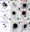 |
Fig. 6 Examples of poststamp images in X-ray (0.5–7 keV), HSC/Subaru-g, and WIRCam/CFHT Ks as labeled. In each panel, the blue circle shows the X-ray source matching radius rmatch (Sec. 3.1). The positions of the HSC-g and WIRCam Ks sources are indicated, respectively, by a green “+” and red “×.” The cyan circle shows the nominal position of the first ID (largest LR). See the description of the table column #11: ID_POS_REF. The numbers on the HSC-g and WIRCam Ks are the numbers for each source based on the distance from the X-ray source’s best-fit position. Full poststamp images are available online (footnote 7). |
4.6 Comments on individual sources
- ANEPD-CXO036:
This is a highly absorbed AGN with a borderline Compton-thick absorption. With a simple absorbed power-law model fit (Sec. 4.3), we obtain log NH = 24.0 (+0.1; −0.2) cm−2 (90% confidence errors) with Γ = 1.8 (fixed). We make spectral analysis using transmitted, scattered, and torus-reflected (XCLUMPY Tanimoto et al. 2019) components. The results will be reported in a future paper.
- ANEPD-CXO083:
The counterpart has a sub-threshold LR value, but the optical spectrum contains a broad Mg II line indicating AGN. The CXO image shows a double peak, indicating that two X-ray sources are blended and recognized as one with a nominal position between two peaks, giving a ~0.9″ offset between the cataloged positions.
- ANEPD-CXO196:
The ID in the catalog is a g = 26.7 HSC source star (Gaia) near the edge of rmatch but it is not likely to be the counterpart. There is an uncatalogued source visible in the WIRCam KS band image with no sign of a source in the HSC-g image closer to the X-ray source nominal position. This is likely to be the true counterpart (See Fig. 6, middle).
- ANEPD-CXO245:
This is a bona fide Compton-thick AGN with double-peaked narrow lines. Even with only 25 source X-ray counts, we can make reasonable X-ray spectral analysis with transmitted, scattered, and torus-reflected (XCLUMPY Tanimoto et al. 2019) components. We refer to Miyaji et al. (2019) for detailed discussions about this source.
- ANEPD-CXO253:
There are two counterpart candidates, both of which have comparably low sub-threshold LR, one 7 × 10⁻⁶ at and the other 4 × 10⁻⁶ separated by 1.8″ and 1.4″ from the X-ray nominal position respectively. The CXO image is weak and has a sign of two peaks. The first candidate has a spectroscopic redshift z = 1.333 with no sign of AGN. We classify it as CLASS=’XAGN’ for its X-ray luminosity.
- ANEPD-CXO256:
There are two Gaia sources that are identification candidates, one is g = 14.7, the other g = 17.3, with separations of 0.5″ and 0.6″ from the X-ray source nominal position respectively.
- ANEPD-CXO398:
The counterpart with spectroscopic red-shift z = 0.75 measured by Eckart et al. (2006) for the same X-ray source (designated by them as CXO-SEXSI J175812.1+664252) is 3″ away from the X-ray source nominal position and its LR value of 0.33 is above our threshold. However, our first candidate counterpart with LR = 5.3, which is fainter (g=24.4), is 0.8″ away from the X-ray source position and has LR = 5.3. We list our first candidate in Table 2.
5 Discussion
5.1 Spectroscopic and photometric redshifts
Among our 376 X-ray source counterparts that have not been classified as Galactic sources, 131 have sufficient quality spectroscopic redshifts (SPECZ_Q=A, AB, B, C, P or X) indicative of extragalactic sources. Oi et al. (2021) used the LE PHARE code (Arnouts et al. 1999; Ilbert et al. 2006) with photometric data in the following 18 optical-IR bands: MegaCam u*, HSC g, r, i, z, y, WIRCam Y, J, Ks, FLAMINGOS J, H, AKARI/IRC N2, N3, N4, WISE W1, W2, and Spitzer/IRAC 3.6 and 4.5 μm to obtain photometric redshifts. In estimating the photometric redshifts, AGN templates are also included. Among our X-ray source counterparts, 78 objects have both spectroscopic and photometric redshifts while 72 objects have photometric redshifts only.
To assess the quality of photometric redshifts for our X-ray-selected AGN sample, we plot photometric versus spectroscopic redshift measurements for the 78 sources that have both. The spectroscopic versus photometric redshift scatter diagram for these 78 objects is shown in Fig. 7. Confirmed broad-line (BL) AGNs (CLASS= ‘AGN1’, see Table 4) and non-BL AGNs (other extragalactic sources) are marked with different symbols. From these sources, we calculate the normalized median absolute deviation (NMAD), defined by σNMAD = 1.48 × median[|zp − zs|/(zs + 1)], where zp and zs are photometric and spectroscopic redshifts, respectively. We also define catastrophic failure rate η, which is conventionally defined as the fraction of objects that have |zp − zs|/(zs + 1) > 0.15. For all the 78 sources that have both spectroscopic and photometric redshifts, we obtain σNMAD = 0.09 and η = 0.28. If we exclude the 31 confirmed broad-line AGNs, we find σNMAD = 0.068 and η = 0.213. For the BL AGNs alone, σNMAD = 0.15 and η = 0.38.
Due to the possibility of AGN variability and the featureless continuum of the AGN component, and the photometric redshifts of AGNs, especially those of luminous type 1 AGNs with optical-IR emission dominated by the AGN component, are subject to systematic errors or even catastrophic failures. Thus, it is natural that these values are worse than those found by Oi et al. (2021) for the whole optical/IR selected sample (σNMAD = 0.06 and η = 0.13 for z < 1.5), even though AGN templates (Salvato et al. 2009; Polletta et al. 2007) are included. Figure 7 shows that a majority of the extreme outliers are z > 1.5 type 1 AGNs that show lower photometric redshift estimates. Thus, for our data, the photometric redshift does not have much use for type-I AGN. However, the photometric redshifts give some estimates of the true redshifts of a majority of the non-BL AGNs. Thus, the redshift estimates from photometric redshifts of Oi et al. (2021) are still useful for those that have other indications of obscured (type II) AGNs and highly obscured AGNs (Herrera-Endoqui et al., in prep.). Those include the X-ray sources that have high ratios of the IR AGN component (obtained from SED fittings) to X-ray (absorption uncorrected) luminosities and those that show absorption in their X-ray spectra.
Figure 8a shows the redshift distributions of the objects with good spectroscopic redshift measurements with SPECZ_Q=A, AB, B, C, P, or X (spec-z sample) that meet our LR threshold. For those with no good spectroscopic redshift measurement, but with a photometric redshift measurement taken from Oi et al. (2021) (photo-z sample), a separate histogram was stacked onto the spec-z sample histogram. To estimate the fraction of X-ray sources that are missing from redshift measurements, we also plot the model-expected redshift distribution of AGNs using the X-ray luminosity function and its evolution from Miyaji et al. (2015) folded with the real Chandra ACIS-I energy response curve and survey solid angle as a function of detection limit in source count rate. The total number of the model-expected AGNs is 352, which is consistent with the number of X-ray sources in our ID catalog presented in Sect. 4.4 that are not known Milky Way objects. The total number of objects that have good spectroscopic measurements is 126 and among those that do not have good spectroscopic redshift measurements, 83 have photometric redshift estimates. This figure shows that a large fraction of sources at z > 0.6 do not yet have redshift information. We also show histograms of objects that are confirmed Milky Way objects, those that have spectroscopic and photometric redshifts, and those that have no redshift measurements/estimates in various quantities: (b) the X-ray (0.5–7 keV) flux, (c) g band magnitude (G_MAG_Gaia if available, G_MAG_HSC otherwise, and (d) Ks magnitude. In panel (b), the expected redshift distribution of the X-ray sources from the X-ray luminosity function by Miyaji et al. (2015) with the survey solid angle versus 0.5–7 keV band count rate relation of our Chandra survey.
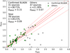 |
Fig. 7 Comparison between spectroscopic redshift (zspec) and photometric redshift (zphot) from Oi et al. (2021) for the 66 sources that have both. Filled circles represent type 1 AGNs (CLASS=XAGN1 in Table 2) while open circles represent non-type 1 objects (CLASS=XAGN/XGAL). The outlier fraction (η) and NMAD (σNMAD) are shown as labels for each of the BL and non-BL objects. The solid red lines represent zspec = zphot and |zphot − zspec|/zspec = 0.05 relations, while red dotted lines correspond to the borders between outlier and non-outlier regimes, corresponding to |zphot − zspec|/zspec = 0.15. |
5.2 Optical and MIR classifications
A comprehensive study for the classifications of galaxies detected by AKARI in MIR identified with a Subaru SCAM-based catalog was made by Hanami et al. (2012) and an early study of the comparison of MIR AGN emission and X-ray finding 28 Compton-thick AGN candidates was presented as a part of K15. We are further conducting revised studies with new datasets including those from HSC, WIRCam, and optical/NIR spectroscopic observations. Kim et al. (2023), Kim et al. (in prep.) are conducting a study of calibrating the PAH emission as a star-formation rate indicator in the ANEPD and ANEPW fields. Among the objects in the sample, 40 match within 1 arc-sec of the Chandra X-ray sources ID presented in this paper. Although not all those objects have good-quality optical spectra, we have identified 8 objects that are good enough for detailed spectral classification. In the standard BPT (Baldwin et al. 1981) diagrams, 7 out of these 8 (88 percent) are classified as “AGN”, with only one being dominated by star formation. We also identified 40 X-ray-emitting galaxies that have very complete spectral energy distributions. These data include all or nearly all of the 9 AKARI MIR bands, which allows us to make a sensitive search for the hot dust continuum known to be produced near a powerful AGN (Edelson & Malkan 2012). Using this more restrictive criterion, we find that 24 of these (60 percent) are identified as having bright AGNs. It is likely that most of the remaining 40 percent also host an AGN, but which is relatively less powerful than its host galaxy, often being classified as a type 2 Seyfert. The BPT classifications and MIR AGNs in this study are indicated in the C0MMENT_OPTIR column in Table 2 enclosed by parentheses with “KM”: followed by the classifications as “BPTAGN”, “BPTSF”, “MIRAGN”, and/or “MIRSF”. Further studies of the search for IR AGNs by the SED fits and identifying obscured AGNs by MIR and X-ray comparisons are the subject of a future paper (Herrera-Endoqui et al. in prep.).
5.3 Current limitations and prospects
While the AKARI IRC photometry and its advantage in finding IR-selected AGNs is a unique feature of the ANEPD field, the supporting multi-wavelength dataset is not as extensive as other premier fields. In particular, the current X-ray data are shallow to take full advantage of the AKARI NEP Deep field data. Thus deeper Chandra data are desired. Unfortunately, due to the thermal constraints imposed by the aging of the Chandra spacecraft, the efficiency of high ecliptic latitude sky has dropped drastically and this has prevented further Chandra observations of this region. The NEP region has been selected for one of the deep fields for the recently launched Euclid, where full deep slitless spectroscopy in the 0.92–1.85 μm using both blue and red grisms (e.g., Euclid Collaboration 2022, 2023; Euclid Collaboration 2024) will be performed and we eventually can expect redshift measurements of a large majority of the X-ray point sources (as well as AKARI IR-selected AGNs) up to ~2.5. Being a part of the Euclid Wide Survey during the first year of the mission, the depths of optical and NIR photometry will reach IE~26.2, YE, JE, and HE~24.5. These will give much improved photometric redshifts.
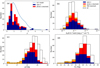 |
Fig. 8 Redshift and flux distribution histograms. (a) Redshift histogram of the spec-z (dark blue histogram) and photo-z (red histogram) samples, where the latter is stacked onto the former. The model expected redshift distribution of AGNs obtained with the X-ray luminosity function model by Miyaji et al. (2015) for our Chandra ANEPD survey is overplotted. (b) X-ray (0.5–7 keV) [SX(0.5–7 keV)] histogram of the X-ray sources in our ID catalog. In addition to the histograms for spec-z and photo-z samples, the distribution of Milky Way (MW) objects is also shown (orange histogram, stacked). The distribution of all objects in our sample is also shown as an un-filled histogram. (c, d) Histograms of g and Ks magnitudes for the X-ray sources that are detected in respective bands. The meaning of colors and styles of the histogram are the same as those in panel (b). |
6 Summary
We present a catalog of optical and NIR counterparts of 403 X-ray sources out of 440 X-ray point sources in the Chandra data in the AKARI NEP Deep Field. These are from the 457 X-ray sources in the main catalog of Krumpe et al. (2015) after certain exclusions (Sec. 4.1). The optical counterparts are searched for among the sources detected in the Subaru HSC g-band as well as Gaia DR3 catalogs, while NIR counterparts are searched for among the sources detected in the CFHT WIRCAM Ks band sources. For this purpose, we developed a novel multi-band X-ray flux-dependent extension of the likelihood ratio (LR) technique. The formulation was developed separately for sources that have both g and Ks detections and those that have detection in only one of these bands. The LR threshold for secure identifications is determined by R = C, where R is the reliability and C is completeness.
Among the 403 first identification candidates, we considered 383 secure in that the LR is above the threshold. The classifications of the 403 identifications are 27 Galactic stars, 132 extragalactic objects with measured spectroscopic redshifts, and 76 extragalactic objects based on photometric redshifts. All the extragalactic sources except 15 objects have AGN luminosities, among which 57 are broad-line (type 1) AGNs. The remaining 173 objects are still unclassified.
The identification catalogs are provided in electronic form for the first optical-IR counterpart candidates and the second and third candidates separately. The catalog also includes the results of the basic X-ray spectral analysis for those that have 20 counts or more in the 0.5–7 keV bands and includes the intrinsic column density and photon index Γ.
We compared the spectroscopic and photometric redshifts for those that have both measurements. For those that have broad emission lines (type I AGNs), the current photometric redshift estimates are not reliable, with σNMAD ~ 0.16 and the outlier fraction of η ~ 39%. Excluding those with broad emission lines, σNMAD ~ 0.06 and η ~ 21%. The field is a part of the Euclid Deep Survey North, where we expect that a very high fraction of the X-ray sources would have spectroscopic redshifts and much improved photometric redshifts.
Data availability
Tables 2, 3 and full Table A.2 are available at the CDS via anonymous ftp to cdsarc.cds.unistra.fr (130.79.128.5) or via https://cdsarc.cds.unistra.fr/viz-bin/cat/J/A+A/689/A83.
Acknowledgements
The scientific results reported in this article are mainly based on observations made by the Chandra X-ray Observatory (OBSIDs: 12925, 12926, 12927, 12928, 12929, 12930, 12931, 12932, 12933, 12934, 12935, 12936, 13244, 10443, and 11999), AKARI, a JAXA project with the participation of ESA and Gran Telescopio Canarias installed at the Spanish Observatorio del Roque de los Muchachos of the Instituto de Astrofísica de Canarias, in the island of La Palma. This paper uses data taken with the MODS spectrographs built with funding from NSF grant AST-9987045 and the NSF Telescope System Instrumentation Program (TSIP), with additional funds from the Ohio Board of Regents and the Ohio State University Office of Research. The authors acknowledge the support by CONACyT Grant Científica Básica #252531, UNAM-DGAPA Grants PAPIIT IN111319 and IN114423. TM acknowledges UNAM-DGAPA (PASPA) for support for his sabbatical leave, during which a significant amount of work for this paper has been done. MK is supported by DLR grant FK2 50 OR 2307. HI is supported by JSPS KAKENHI, Grant-in-Aid for Scientific Research (C) 23K03465. HSH acknowledges the support of the National Research Foundation of Korea (NRF) grant funded by the Korean government (MSIT) (No. 2021R1A2C1094577). TG acknowledges the support of the National Science and Technology Council of Taiwan through grants 112-2112-M-007-013, and 112-2123-M-001-004. We thank Hermann Brunner for his early work in X-ray source detection.
Appendix A Gran Telescopio Canarias (GTC) and Large Binocular Telescope (LBT) spectroscopy in the AKARI NEP Deep Field
A.1 The GTC spectroscopic program
Given the multiwavelength coverage currently available for the AKARI NEP Deep Field, ranging from Chandra X-rays to AKARI MIR and Herschel FIR, we carried out a spectroscopic survey of MIR and X-ray selected AGN. In particular, we aimed to quantify the existence of highly obscured AGNs, including Compton-thick (CT) AGNs. The purpose of the spectroscopy was to obtain accurate redshifts and identify AGN signatures of X-ray and MIR AGNs to help calibrate the LX/LIR,AGN estimate as well as to help the X-ray stacking analysis in the rest frame, to detect the integrated X-ray Fe K-α line, which has large equivalent widths in CT AGNs. Thus, we put priorities on strong CT AGN candidates and type 1 AGN candidates. We also put priorities on targets with high X-ray and/or MIR AGN-component fluxes.
Multi-object-spectroscopy of optical counterparts of both Chandra X-ray sources as AKARI MIR sources were made using the Optical System for Imaging and low-intermediate Resolution Integrated Spectroscopy (OSIRIS) of the Gran Telescopio Canarias (GTC). We obtained the data from one cycle with the long-slit mode performed in 2010 (GTC13-10AMEX) and four observation cycles with the Multi-object spectroscopy mode from 2014 to 2017 (GTC7-14AMEX, GTC4-15AMEX, GTC4-15BMEX and GTC4-17AMEX). Considering the Field of View (FOV) of OSIRIS is 7.5 × 6 arcmin2, some of the pointing were located inside the same area already registered to repeat the observation of some objects and also include new ones. This multi-cycle approach was applied to maximize the number of galaxies observed by area and obtain deep observation for the faintest objects but with scientific meaning. Figure A.1 shows the pointings of the masks used in the AKARI NEP Deep Field. In this figure, boxes represent the area covered by OSIRIS, while small circles show the objects observed. Each observation cycle is shown with a different color (GTC7-2014AMEX in green, GTC4-15AMEX in red, GTC4-15BMEX in blue and GTC4-17AMEX in black). The regions close to the center and upper right of the field were not observed due to other spectroscopic campaigns also observing the field, such as DEIMOS/KECK (PI: M. Malkan). We concentrated our observations in the remaining regions of the field but in particular in the area where Chandra observations were deeper (bottom left area of the field; see Fig. 1 of K15), pointing several times to that region.
The OSIRIS FOV allows the acquisition of ~30 spectra without overlap between them. In the observations, the R500B and R500R grisms were used for all cycles except the last year (where only R500B grism was utilized), giving dispersions of 3.54 and 4.88 Å/pix, respectively. With these grisms, the spectral coverages were from 360 to 700 nm for R500B and from 500 to 1000 nm for R500R, respectively. However, in some cases, the R500B grism practically provided good spectra from 360 to 1000 nm, but with a lower sensitivity toward redder wavelengths, providing thus two measures of features for the same object. The slit width adopted in the observations was 1.2 arcsec, which is a value higher than the average seeing of the whole run (1 arcsec), while the average slit length was 5 arcsec. Typical integration times of ~700 s and ~1100 s were used for R500B and R500R grisms, respectively, to reach a signal-to-noise ratio (S/N) over 3 in the spectra obtained. Table A.1 summarizes the observation details used in our multi-cycle strategy. Usual calibration frames were acquired during the run plus standard star spectra to make flux calibrations.
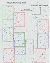 |
Fig. A.1 Mask positions of OSIRIS/GTC in the AKARI NEP Deep Field. Boxes show the OSIRIS coverage area in the different pointings used. Small circles show the objects selected for spectroscopy in each mask. Colors indicate the observation cycle in which each mask and target were used; green for GTC7-14AMEX, red for GTC4-15AMEX, blue for GTC4-15BMEX, and black for GTC4-17AMEX cycles, respectively. |
The data reduction process was carried out via the gtcmos package8, which works in IRAF. Before using this package, the OSIRIS images composed of two CCDs with a gap and a slight shift and rotation between them were combined into a single mosaic frame with their pixel coordinates geometrically corrected. This process was performed via the mosaic2x2_v2 task available on the GTC website. Then, the images were combined and bias subtracted using standard routines of IRAF. The arc line identification, wavelength calibration, and sky subtraction steps were carried out with the omidentify, omreduce, and omskysub routines, respectively, to obtain the calibrated 2D spectra. The 1D spectra were extracted via the omextract routine, while the standard stars were extracted with the apall routine. Finally, the flux calibration process was performed with the standard, sensfunction, and calibrate routines, also within IRAF.
Table A.2 summarizes the measured spectroscopic redshifts and identified spectroscopic features for the Chandra X-ray selected sources and other sources in the ANEPD field observed with OSIRIS/GTC. Each column gives the following information:
- #1:
ObjectID – Object Identifier adopted from Krumpe et al. (2015) for Chandra X-ray sources. For non-X-ray sources, the ID numbers marked by a ‘+’ is from an internal z′-based catalog Hanami et al. (2012), ‘*’ from Oi et al. (2014), and no mark from Murata et al. (2013).
- #2:
RA – unit: deg – Right Ascension of the object position.
- #3:
DEC – unit: deg – Declination of the object position.
- #4:
TEL/INSTR – Telescope/Instrument
- #5:
MaskID – Mask ID. See Table A.1.
- #6:
z_spec Spectroscopic redshift estimated for the object.
- #7:
Q – Quality Flag of the measured redshift. Q indicates the quality of the redshift estimates, discriminating them according to how many features were used to obtain a redshift. The Q flag of “A” means that at least three emission lines were identified (without accounting absorption lines), “B” signifies that only one or two emission lines were recognized (again, without accounting absorption lines), “C” value indicates that only one emission line and no absorption lines were distinguished, and “D” denotes that the redshift estimate is not sufficiently reliable. In addition, the (*) symbol attached to the Q value means that different observations confirm the measured redshift.
- #8:
CLASS – Object Class revealed by the optical spectroscopy. See Table 4 for classifications of the X-ray sources. Those that are not detected in X-rays are indicated by the same nomenclature without preceding “X”.
- #9:
SEP – unit: arcsec- Distance between the slitlet position and the catalog object position, from where the ObjectID had its origin.
- #10:
COMMENTS – Comments about the features revealed by the spectrum.
A.2 The LBT spectroscopy
The LBT observations were obtained with the Multi-Object Double Spectrograph (MODS, Pogge et al. 2010) instruments. At the time of taking the data, only one of the two main mirrors was equipped with a MODS (specifically the SX version). The spectrograph operates in the 3200 to 10,000 Å range with a 6 × 6 arcmin field of view. Using user-designed laser-machine-cut multi-object masks, the light is split into red and blue-optimized spectrograph channels. The cross-over region is ~5700 Å. For the blue channel, the Grating G400L was used, while the red channel used G670L. The data for both masks, including a total of 37 slits, were collected on May 12 and 13, 2016 with an integration time of 4 × 1200 s for each mask.
Standard calibration files for each mask were used. This included biases, flat-field, wavelength-calibration arc lamps, and standard star observations for flux calibration. The data reduction was a two-stage process. First, using modsCCDRed9, bias and flat-flied corrections were applied. Then, the data were further reduced with scripts written for the reduction of multi-object spectroscopy instruments in ESO-MIDAS. This reduction includes cosmic filtering of the science images, wavelength calibration, weighted extraction of 1D spectra, creation of error spectra, and co-adding the single spectra. The log of observations of the LBT spectroscopy is also shown in Table A.1. The spectroscopic redshifts and identified features from our LBT observations are also included in Table A.2.
Log of Observations
Spectroscopic redshifts obtained in our spectroscopic programs with OSIRIS/GTC and LBT/MODS.
References
- Aihara, H., AlSayyad, Y., Ando, M., et al. 2019, PASJ, 71, 114 [Google Scholar]
- Arnouts, S., Cristiani, S., Moscardini, L., et al. 1999, MNRAS, 310, 540 [Google Scholar]
- Baldwin, J. A., Phillips, M. M., & Terlevich, R. 1981, PASP, 93, 5 [Google Scholar]
- Brusa, M., Zamorani, G., Comastri, A., et al. 2007, ApJS, 172, 353 [NASA ADS] [CrossRef] [Google Scholar]
- Burgarella, D., Mazyed, F., Oi, N., et al. 2019, PASJ, 71, 12 [CrossRef] [Google Scholar]
- Churei, S. 2013, Master’s thesis, Tokyo Institute of Technology, Japan [Google Scholar]
- Civano, F., Elvis, M., Brusa, M., et al. 2012, ApJS, 201, 30 [Google Scholar]
- Civano, F., Marchesi, S., Comastri, A., et al. 2016, ApJ, 819, 62 [Google Scholar]
- Díaz Tello, J., Miyaji, T., Ishigaki, T., et al. 2017, A&A, 604, A14 [NASA ADS] [CrossRef] [EDP Sciences] [Google Scholar]
- Eckart, M. E., Stern, D., Helfand, D. J., et al. 2006, ApJS, 165, 19 [NASA ADS] [CrossRef] [Google Scholar]
- Edelson, R., & Malkan, M. 2012, ApJ, 751, 52 [NASA ADS] [CrossRef] [Google Scholar]
- Euclid Collaboration (Scaramella, R., et al.) 2022, A&A, 662, A112 [NASA ADS] [CrossRef] [EDP Sciences] [Google Scholar]
- Euclid Collaboration (Gabarra, L., et al.) 2023, A&A, 676, A34 [NASA ADS] [CrossRef] [EDP Sciences] [Google Scholar]
- Euclid Collaboration (Lusso, E., et al.) 2024, A&A, 685, A108 [NASA ADS] [CrossRef] [EDP Sciences] [Google Scholar]
- Gioia, I. M., Henry, J. P., Mullis, C. R., et al. 2003, ApJS, 149, 29 [NASA ADS] [CrossRef] [Google Scholar]
- Hanami, H., Ishigaki, T., Fujishiro, N., et al. 2012, PASJ, 64, 70 [NASA ADS] [Google Scholar]
- Huang, T.-C., Matsuhara, H., Goto, T., et al. 2021, MNRAS, 506, 6063 [NASA ADS] [CrossRef] [Google Scholar]
- Ilbert, O., Arnouts, S., McCracken, H. J., et al. 2006, A&A, 457, 841 [NASA ADS] [CrossRef] [EDP Sciences] [Google Scholar]
- Kalberla, P. M. W., Burton, W. B., Hartmann, D., et al. 2005, A&A, 440, 775 [NASA ADS] [CrossRef] [EDP Sciences] [Google Scholar]
- Kim, S. J., Lee, H. M., Matsuhara, H., et al. 2012, A&A, 548, A29 [NASA ADS] [CrossRef] [EDP Sciences] [Google Scholar]
- Kim, H. K., Malkan, M., Oi, N., et al. 2020, in Panchromatic Modelling with Next Generation Facilities, 341, eds. M. Boquien, E. Lusso, C. Gruppioni, & P. Tissera, 279 [Google Scholar]
- Kim, S. J., Oi, N., Goto, T., et al. 2021, MNRAS, 500, 4078 [Google Scholar]
- Kim, H., Malkan, M., & Akari Nep Team 2023, in American Astronomical Society Meeting Abstracts, 55, 144.03D [Google Scholar]
- Kim, T., Hwang, H. S., Ho, S. C.-C., et al. 2024, ApJS, submitted [Google Scholar]
- Krumpe, M., Miyaji, T., Brunner, H., et al. 2015, MNRAS, 446, 911 [NASA ADS] [CrossRef] [Google Scholar]
- Laigle, C., McCracken, H. J., Ilbert, O., et al. 2016, ApJS, 224, 24 [Google Scholar]
- Marchesi, S., Civano, F., Elvis, M., et al. 2016, ApJ, 817, 34 [Google Scholar]
- Matsuhara, H., Shibai, H., Onaka, T., & Usui, F. 2005, Adv. Space Res., 36, 1091 [NASA ADS] [CrossRef] [Google Scholar]
- Matsuhara, H., Wada, T., Matsuura, S., et al. 2006, PASJ, 58, 673 [NASA ADS] [Google Scholar]
- Miyaji, T., Hasinger, G., Salvato, M., et al. 2015, ApJ, 804, 104 [Google Scholar]
- Miyaji, T., Herrera-Endoqui, M., Krumpe, M., et al. 2019, ApJ, 884, L10 [NASA ADS] [CrossRef] [Google Scholar]
- Miyaji, T., & Akari Nep Survey Team 2020, in Panchromatic Modelling with Next Generation Facilities, 341, eds. M. Boquien, E. Lusso, C. Gruppioni, & P. Tissera, 172 [Google Scholar]
- Murata, K., Matsuhara, H., Wada, T., et al. 2013, A&A, 559, A132 [NASA ADS] [CrossRef] [EDP Sciences] [Google Scholar]
- Ohyama, Y., Wada, T., Matsuhara, H., et al. 2018, A&A, 618, A101 [NASA ADS] [CrossRef] [EDP Sciences] [Google Scholar]
- Oi, N., Matsuhara, H., Murata, K., et al. 2014, A&A, 566, A60 [NASA ADS] [CrossRef] [EDP Sciences] [Google Scholar]
- Oi, N., Goto, T., Malkan, M., Pearson, C., & Matsuhara, H. 2017, PASJ, 69, 70 [NASA ADS] [CrossRef] [Google Scholar]
- Oi, N., Goto, T., Matsuhara, H., et al. 2021, MNRAS, 500, 5024 [Google Scholar]
- Pearson, C., Barrufet, L., Campos Varillas, M. d. C., et al. 2019, PASJ, 71, 13 [NASA ADS] [CrossRef] [Google Scholar]
- Pogge, R. W., Atwood, B., Brewer, D. F., et al. 2010, SPIE Conf. Ser., 7735, 77350A [Google Scholar]
- Polletta, M., Tajer, M., Maraschi, L., et al. 2007, ApJ, 663, 81 [NASA ADS] [CrossRef] [Google Scholar]
- Rumbaugh, N., Lemaux, B. C., Tomczak, A., et al. 2017, MNRAS, 466, 496 [NASA ADS] [CrossRef] [Google Scholar]
- Salvato, M., Hasinger, G., Ilbert, O., et al. 2009, ApJ, 690, 1250 [CrossRef] [Google Scholar]
- Salvato, M., Buchner, J., Budavári, T., et al. 2018, MNRAS, 473, 4937 [Google Scholar]
- Salvato, M., Wolf, J., Dwelly, T., et al. 2022, A&A, 661, A3 [NASA ADS] [CrossRef] [EDP Sciences] [Google Scholar]
- Shim, H., Im, M., Ko, J., et al. 2013, ApJS, 207, 37 [NASA ADS] [CrossRef] [Google Scholar]
- Shogaki, A. 2018, Master’s thesis, Kwansei Gakuin University, Japan [Google Scholar]
- Sutherland, W., & Saunders, W. 1992, MNRAS, 259, 413 [Google Scholar]
- Takagi, T., Matsuhara, H., Goto, T., et al. 2012, A&A, 537, A24 [NASA ADS] [CrossRef] [EDP Sciences] [Google Scholar]
- Tanaka, M., Hasinger, G., Silverman, J. D., et al. 2017, arXiv e-prints [arXiv:1706.00566] [Google Scholar]
- Tanimoto, A., Ueda, Y., Odaka, H., et al. 2019, ApJ, 877, 95 [Google Scholar]
- Wada, T., Matsuhara, H., Oyabu, S., et al. 2008, PASJ, 60, S517 [NASA ADS] [CrossRef] [Google Scholar]
- Wang, T.-W., Goto, T., Kim, S. J., et al. 2020, MNRAS, 499, 4068 [NASA ADS] [CrossRef] [Google Scholar]
- White, G. J., Pearson, C., Braun, R., et al. 2010, A&A, 517, A54 [NASA ADS] [CrossRef] [EDP Sciences] [Google Scholar]
Developed by Divakara Mayya at INAOE, Puebla, Mexico. Available in https://www.inaoep.mx/~ydm/gtcmos/gtcmos.html
All Tables
Spectroscopic redshifts obtained in our spectroscopic programs with OSIRIS/GTC and LBT/MODS.
All Figures
|
Fig. 1 Number counts inin ANEPD. (a) Number counts dN(n)/dm (deg−2 mag−1) of g-band sources in the AKARI NEP Deep Field (within the Chandra field, from Gaia and HSC) and the COSMOS field (HSC). (b) Number counts for the Ks band. Both come from CFHT/WIRCam. |
| In the text | |
|
Fig. 2 Histograms for sources detected in both g and Ks bands for template sample with models. (a) Histogram showing the dN/d log SX distribution of the template sample of X-ray sources that have both g and Ks, constructed from the COSMOS Legacy survey. The curve shows the best-fit model. (b, c) Histograms of log SX + 0.4g distribution of the template sample and the best-fit model (curve) for the high and low flux regimes respectively as labeled. (d, e) Same as (b, c) for the g − Ks distributions. In all panels, SX is the 0.5–7 keV flux in units of erg s−1 cm−2. |
| In the text | |
|
Fig. 3 Histograms for sources detected in g, but not detected in Ks for template sample with models. (a) Histogram showing the dN/d log SX distribution of the template sample of X-ray sources that are detected in HSC g-band, but not in CFHT Ks (depth matched with AKARI NEP Deep Field; See text), constructed from the COSMOS Legacy survey. The curve shows the best-fit model. (b, c) Histograms of log SX + 0.4 g distribution of the template sample and the best-fit model. |
| In the text | |
 |
Fig. 4 Same as Fig. 3, except that this is for KS band detected g-band undetected sources. |
| In the text | |
|
Fig. 5 Unidentified source fraction and reliability-completeness analysis. (a) Fraction of X-ray sources that have no candidate in any of our HSC-g, Gaia-g or WIRCam-Ks catalog as a function of SX with the histogram binsize of dex in flux. Approximate 1σ errors are also shown. (b) Reliability (R), completeness (C) and (R + C)/2 curves as a function of log LRth, as labeled. |
| In the text | |
|
Fig. 6 Examples of poststamp images in X-ray (0.5–7 keV), HSC/Subaru-g, and WIRCam/CFHT Ks as labeled. In each panel, the blue circle shows the X-ray source matching radius rmatch (Sec. 3.1). The positions of the HSC-g and WIRCam Ks sources are indicated, respectively, by a green “+” and red “×.” The cyan circle shows the nominal position of the first ID (largest LR). See the description of the table column #11: ID_POS_REF. The numbers on the HSC-g and WIRCam Ks are the numbers for each source based on the distance from the X-ray source’s best-fit position. Full poststamp images are available online (footnote 7). |
| In the text | |
|
Fig. 7 Comparison between spectroscopic redshift (zspec) and photometric redshift (zphot) from Oi et al. (2021) for the 66 sources that have both. Filled circles represent type 1 AGNs (CLASS=XAGN1 in Table 2) while open circles represent non-type 1 objects (CLASS=XAGN/XGAL). The outlier fraction (η) and NMAD (σNMAD) are shown as labels for each of the BL and non-BL objects. The solid red lines represent zspec = zphot and |zphot − zspec|/zspec = 0.05 relations, while red dotted lines correspond to the borders between outlier and non-outlier regimes, corresponding to |zphot − zspec|/zspec = 0.15. |
| In the text | |
|
Fig. 8 Redshift and flux distribution histograms. (a) Redshift histogram of the spec-z (dark blue histogram) and photo-z (red histogram) samples, where the latter is stacked onto the former. The model expected redshift distribution of AGNs obtained with the X-ray luminosity function model by Miyaji et al. (2015) for our Chandra ANEPD survey is overplotted. (b) X-ray (0.5–7 keV) [SX(0.5–7 keV)] histogram of the X-ray sources in our ID catalog. In addition to the histograms for spec-z and photo-z samples, the distribution of Milky Way (MW) objects is also shown (orange histogram, stacked). The distribution of all objects in our sample is also shown as an un-filled histogram. (c, d) Histograms of g and Ks magnitudes for the X-ray sources that are detected in respective bands. The meaning of colors and styles of the histogram are the same as those in panel (b). |
| In the text | |
|
Fig. A.1 Mask positions of OSIRIS/GTC in the AKARI NEP Deep Field. Boxes show the OSIRIS coverage area in the different pointings used. Small circles show the objects selected for spectroscopy in each mask. Colors indicate the observation cycle in which each mask and target were used; green for GTC7-14AMEX, red for GTC4-15AMEX, blue for GTC4-15BMEX, and black for GTC4-17AMEX cycles, respectively. |
| In the text | |
Current usage metrics show cumulative count of Article Views (full-text article views including HTML views, PDF and ePub downloads, according to the available data) and Abstracts Views on Vision4Press platform.
Data correspond to usage on the plateform after 2015. The current usage metrics is available 48-96 hours after online publication and is updated daily on week days.
Initial download of the metrics may take a while.